Stimulus-Dependent Auditory Tuning Results in Synchronous Population Coding of Vocalizations in the Songbird Midbrain

Abstract

Physiological studies in vocal animals such as songbirds indicate that vocalizations drive auditory neurons particularly well. But the neural mechanisms whereby vocalizations are encoded differently from other sounds in the auditory system are unknown. We used spectrotemporal receptive fields (STRFs) to study the neural encoding of song versus the encoding of a generic sound, modulation-limited noise, by single neurons and the neuronal population in the zebra finch auditory midbrain. The noise was designed to match song in frequency, spectrotemporal modulation boundaries, and power. STRF calculations were balanced between the two stimulus types by forcing a common stimulus subspace. We found that 91% of midbrain neurons showed significant differences in spectral and temporal tuning properties when birds heard song and when birds heard modulation-limited noise. During the processing of noise, spectrotemporal tuning was highly variable across cells. During song processing, the tuning of individual cells became more similar; frequency tuning bandwidth increased, best temporal modulation frequency increased, and spike timing became more precise. The outcome was a population response to song that encoded rapidly changing sounds with power and precision, resulting in a faithful neural representation of the temporal pattern of a song. Modeling responses to song using the tuning to modulation-limited noise showed that the population response would not encode song as precisely or robustly. We conclude that stimulus-dependent changes in auditory tuning during song processing facilitate the high-fidelity encoding of the temporal pattern of a song.

Introduction

Speech and birdsong are characterized by spectrotemporal complexity (Chi et al., 1999; Singh and Theunissen, 2003). Other acoustic communication signals that may be less rich in the spectral domain are highly temporally structured (Suga, 1989; Bass and McKibben, 2003; Kelley, 2004; Mason and Faure, 2004). Correspondingly, behavioral and physiological studies suggest a strong relationship between the accurate perception of communication sounds and temporal auditory processing (Tallal et al., 1993; Shannon et al., 1995; McAnally and Stein, 1996; Wright et al., 1997; Woolley and Rubel, 1999; Escabi et al., 2003; Ronacher et al., 2004; Marsat and Pollack, 2005; Woolley et al., 2005). Natural sounds such as vocalizations and/or sounds that are “natural-like” evoke more informative responses (e.g., higher information rates) from auditory neurons (Rieke et al., 1995; Machens et al., 2001; Escabi et al., 2003; Hsu et al., 2004). But how single neurons and neuronal populations code natural sounds differently from other sounds such as noise is not known. To address this issue, we compared the encoding of a behaviorally important natural sound and a behaviorally neutral synthetic sound by the same auditory neurons.

In bats and frogs, the auditory midbrain has been implicated in the specialized processing of vocal signals (Pollak and Bodenhamer, 1981; Rose and Capranica, 1983, 1985; Casseday et al., 1994; Dear and Suga, 1995; Mittmann and Wenstrup, 1995) as well as temporal information (for review, see Covey and Casseday, 1999) (Alder and Rose, 2000). In the bat auditory midbrain (inferior colliculus), many neurons are selectively sensitive to the frequencies of a bat’s species-specific echolocation calls (Pollak and Bodenhamer, 1981). In the anuran midbrain (torus semicircularis), single neurons respond specifically to amplitude modulation rates that are related to species-typical vocalizations (Rose and Capranica, 1985). The response properties of neurons in the songbird auditory midbrain, the mesencephalicus lateralis dorsalis (MLd), are also highly sensitive to the temporal properties of sound (Woolley and Casseday, 2004, 2005) and give highly informative responses to vocalizations (Hsu et al., 2004; Woolley et al., 2005). In an effort to understand how song may be encoded differently from other sounds in the songbird auditory midbrain, we examined the responses of single neurons and the neuronal population in the MLd of adult male zebra finches to song and to modulation-limited (ml) noise. ml noise is a behaviorally meaningless sound that was designed to match song in frequency range, maximum spectral and temporal modulations, and power. Responses were analyzed in terms of linear frequency and temporal tuning using normalized reverse correlation to obtain spectrotemporal receptive fields (STRFs). STRFs obtained from responses to both song and ml noise were used to predict the responses of single neurons and of the neuronal population to songs. The song STRFs and the ml noise STRFs and their associated predictions were compared to understand how the same neurons may encode a behaviorally meaningful sound, song, and a synthetic sound differently.

Materials and Methods

Animals and experimental design

All animal procedures were approved by the Animal Care and Use Committee at the University of California, Berkeley. Twenty-one adult (>120 d of age) male zebra finches (Taenopygia guttata) were used. All birds were bred and raised at the University of California, Berkeley.

We recorded the electrophysiological responses of single units in the auditory midbrain region, MLd, to two classes of sounds: zebra finch songs and a noise stimulus called ml noise (see details below). Responses were analyzed using a normalized reverse correlation procedure to obtain a STRF for the responses of a neuron to each stimulus type. An STRF shows the linear time/frequency tuning properties of a neuron as it is processing complex acoustic stimuli. Classical measures such as characteristic frequency, frequency tuning bandwidth, temporal response pattern, best temporal modulation frequency, and spike latency can be obtained from the STRF. A separate STRF was obtained for responses to each of the two stimulus types (song and ml noise). We then analyzed the two STRFs from the same neuron for differences in tuning, depending on the stimulus type.

To examine how tuning differences affect population coding of complex sounds, we convolved STRFs with each individual stimulus (e.g., one sample of song) to obtain predicted responses to each stimulus. Those predictions were then averaged across all cells to get a predicted population response to each individual stimulus. Those population predictions were compared with the actual population responses to each stimulus, which were calculated by averaging the actual responses of all neurons to a particular stimulus. For each song stimulus, predicted population responses were calculated using both the song STRFs and the ml noise STRFs. This analysis was designed to examine the effects of stimulus-dependent tuning differences on population coding. Using this approach, we were able to estimate how tuning differences affected the encoding of song in midbrain neurons.

Stimuli

Two stimuli, zebra finch song and ml noise, were used (Fig. 1). The zebra finch song stimulus set consisted of song samples from 20 adult male zebra finches (age, >120 d). Each song sample (∼2 s in duration) was recorded in a sound-attenuated chamber (Acoustic Systems, Austin, TX), digitized at 32 kHz (TDT Technologies, Alachua, FL), and frequency filtered at 250 and 8000 Hz (Fig. 1A). The synthetic stimulus, ml noise, was designed to have a flat power spectrum between 250 and 8000 Hz, and the absolute power level was adjusted so that the peak value in the power spectrum of song (found ∼3.5 kHz) matched the power level of the ml noise (Fig. 1B,C). The absolute power of both stimuli were adjusted so that peak levels in song stimuli were at ∼70 dB sound pressure level (SPL).

Figure 1.

Stimuli. A, Top, A spectrogram of song. Intensity is indicated by color. Red is high amplitude, and blue is low amplitude. Bottom, The amplitude waveform showing the temporal pattern of the song. B, Top, A spectrogram of the synthetic stimulus, modulation-limited noise. Bottom, The amplitude waveform showing the temporal pattern of the ml noise. C, The one-dimensional (1D) power spectra of song (blue) and ml noise (red). The stimuli have the same frequency range and peak power. D, The two-dimensional (2D) power spectra for song and ml noise, also called modulation power spectra. The ml noise was designed to match the maximum spectral and temporal modulations of song.

The ml noise was designed to share the same maximum and minimum spectral and temporal modulations as song (Fig. 1D). This stimulus is akin to white noise that has been limited in spectrotemporal modulations. Spectral and temporal modulations describe the oscillations in power across time and frequency that characterize the dynamic properties of complex sounds and are visualized in a spectrogram (Singh and Theunissen, 2003; Woolley et al., 2005). Spectral modulations are oscillations in power across the frequency spectrum, such as harmonic stacks, and are measured in cycles per kilohertz. Temporal modulations are oscillations in power over time and are measured in hertz. Zebra finch songs contain a limited set of spectral and temporal modulations that, combined with the phase information, characterize the unique sounds of zebra finch song (Fig. 1A, top; D, left). The modulations that characterize complex sounds are plotted using a modulation power spectrum, showing the amount of energy (color axis) as a function of temporal modulation frequency (x-axis) and spectral modulation frequency (y-axis) in an ensemble of sounds. The spectral modulation frequencies found in zebra finch song range between 0 and ∼2 cycles (cyc)/kHz (Fig. 1D, left). The temporal modulation frequencies in song range between 0 and ∼50 Hz. The ml noise was created by uniformly sampling spectrotemporal modulations ranging between 0 and 2 cyc/kHz spectral modulation and 0–50 Hz temporal modulation (Fig. 1D, right).

To generate the ml noise, we calculated the spectrotemporal log envelope function of the sound (i.e., its spectrogram in logarithmic units) as a sum of ripple sounds. Ripples are broadband sounds that are the auditory equivalents of sinusoidal gratings typically used in vision research. This sum of ripples can be written as follows:

where φ_i is the modulation phase, and ω_t,i and ω_x,i are the spectral and temporal frequency modulations for the ith ripple component, and S(t, x) is the zero mean log envelope of the frequency band x. We used N = 100 ripples. The modulation phase was random, taken from a uniform distribution. The spectral and temporal modulation frequencies were sampled randomly from a uniform distribution of modulations bounded by 50 Hz and 2 cyc/kHz (Fig. 1D). The frequency x was sampled uniformly between 250 and 8000 Hz (Fig. 1C).

The actual envelope used to generate the sounds was then obtained from S(t,x) by adding the DC level and modulation depth obtained from the log envelope of song. The envelope is written as follows:

where A(x_Peak) is the DC level of the log amplitude envelope at the frequency at which it is the largest in song; σ(x) is the SD across time of the log envelope for a frequency, x, also calculated for song; and σ_S(x) is the SD obtained from the generated amplitudes S(t, x). Therefore, the mean amplitude (and thus intensity) in each frequency band was constant and given by the peak of the log amplitude envelope in song; ml noise had a flat power spectrum between 250 and 8000 Hz with levels that matched the peak of the power spectrum of song found at x_Peak ∼ 3.5 kHz. The modulation depth (in log units) in each frequency band was set to the average modulation depth found in song across all frequency bands. The sound pressure waveform was then obtained by taking the exponential of the normalized log amplitude envelope, S_Norm(t, x), and using a spectrographic inversion routine (Singh and Theunissen, 2003).

Surgery

Two days before recording, a bird was anesthetized with Equithesin (0.03 ml, i.m., of the following: 0.85 g of chloral hydrate, 0.21 g of pentobarbital, 0.42 g of MgSO₄, 8.6 ml of propylene glycol, and 2.2 ml of 100% ethanol to a total volume of 20 ml with H₂O). The bird was then placed in a custom stereotaxic with ear bars and a beak holder. Lidocaine (2%) was applied to the skin overlying the skull, and a midline incision was made. A metal pin was fixed to the skull with dental cement. The bird was then allowed to recover for 2 d.

On the day of recording, the bird was anesthetized with three injections of 20% urethane (three intramuscular injections; 30 ml each; 30 min apart) and placed in the stereotaxic. Urethane, at this dose, achieves a level of profound anesthesia without complete loss of consciousness. The bird’s head was immobilized by attaching the metal pin cemented to the bird’s skull to a customized holder mounted on the stereotaxic. Lidocaine was applied to the skin overlying the skull region covering the optic lobe. After lidocaine application, a small incision was made in the skin over the skull covering the optic tectum. A small opening was made in the skull overlying the optic tectum, and the dura was resected from the surface of the brain.

Electrophysiology

Neural recordings were conducted in a sound-attenuated chamber (Acoustic Systems). The bird was positioned ∼20 cm in front of a Bose 101 speaker so that the bird’s beak was centered both horizontally and vertically with the center of the speaker cone. The output of the speaker was measured before each experiment with a Radio Shack electret condenser microphone (33-3013) and custom software to ensure a flat response (±5 dB) from 250 to 8000 Hz. Sound levels were checked with a B&K (Norcross, GA) sound level meter [root mean square (RMS) weighting B; fast] positioned 25 cm in front of the speaker at the bird’s head. Body temperature was continuously monitored and adjusted to between 38 and 39°C using a custom-designed heater with a thermistor placed under a wing and a heating blanket placed under the bird.

Recordings were obtained using epoxy-coated tungsten electrodes (0.5–7.0 MΩ; Frederick Haer, Bowdoinham, ME; or A-M Systems, Carlsborg, WA). Electrodes were advanced into the brain with a stepping microdrive at 0.5 μm steps (Newport, Fountain Valley, CA). The extracellular signal was obtained with a Neuroprobe amplifier (A-M Systems; X100 gain; high-pass f_c, 300 Hz; low-pass f_c, 5 kHz), displayed on a multichannel oscilloscope (TDS 210; Tektronix, Wilsonville, OR), and monitored on an audio amplifier/loudspeaker (Grass AM8). Single-unit spike arrival times were obtained by thresholding the extracellular recordings with a window discriminator and were logged on a Sun computer running custom software (<1 ms resolution).

Pure tones (250–8000 Hz), zebra finch songs, ml noise, and white noise were used as search stimuli. If the response to any of these stimuli was significantly different from the baseline firing rate or the response was clearly time locked to some portion of the stimulus, then we acquired 10 trials of data to each of 20 zebra finch songs and 10 ml noise stimuli. Presentation of the stimuli was random within a trial. Two seconds of background spontaneous activity was recorded before the presentation of each stimulus. A random interstimulus interval with a uniform distribution between 4 and 6 s was used. At the end of a penetration, one to three electrolytic lesions (100 μA for 5 s) were made to verify the recording sites for that penetration. Lesions were made well outside of any auditory areas unless it was the last penetration.

Histology

After recording, the bird was deeply anesthetized with Nembutal and transcardially perfused with 0.9% saline followed by 3.7% formalin in 0.025 m phosphate buffer. The skullcap was removed and the brain was postfixed in formalin for at least 5 d. The brain was then cryoprotected in 30% sucrose. Coronal sections (40 μm) were cut on a freezing microtome and divided into two series. Sections were mounted on gelatin-subbed slides, and one series was stained with cresyl violet and the other with silver stain. Electrolytic lesions were visually identified, and the distance between two lesions within the same electrode track was used to calibrate depth measurements and reconstruct the locations of recording sites.

Data analysis

STRF calculation.

A normalized reverse correlation analysis was used to determine the relationship between the stimulus and response. This analysis yields the STRF, which is a linear model of the auditory tuning properties of a neuron. The STRF calculation entails three steps. First, a spike-triggered average (STA) is generated by doing a reverse correlation between the spectrogram of a sound stimulus (e.g., a sample of song) and the poststimulus time histogram (PSTH) of the responses to that stimulus (Fig. 2A). The PSTH is the summed responses to 10 presentations of the same stimulus (10 trials). Second, the correlations in the stimulus are removed from the spike-triggered average by dividing the spike-triggered average by the autocorrelation of the stimulus. Third, a regularization procedure (see below) is used to reduce the number of stimulus parameters that are needed to obtain the STRF, given the amount of data and the noise in the response. Once the STRF is obtained, it is validated on data that were not used in the STRF calculation by using the STRF to predict the response to a stimulus and comparing that predicted response to the actual recorded response. The similarity between the predicted response given by the STRF and the actual response, measured using correlation coefficients, provides the measure of how well the linear STRF captures the tuning of a neuron. Previous descriptions of this STRF methodology are in Theunissen et al. (2000, 2001, 2004).

Figure 2.

Calculation of the STRF. A, A schematic illustrating how the song shown in a spectrogram is reverse correlated with the PSTH to obtain the STRF for the cell (after normalization and regularization). Red represents excitation. Blue represents inhibition. Green represents the mean firing rate. B, A plot showing the number of eigenvectors that are needed to describe the stimulus subspace for each temporal frequency. Each colored line shows the number of eigenvectors for a different threshold (tolerance) value. The tolerance value determines the threshold for acceptable eigenvalues as a percentage of the maximum eigenvalue and therefore determines the acoustic subspace. The total number of dimensions (STRF parameters) that are used is shown in parentheses. C, The goodness of fit of the STRF calculated with a varying number of dimensions as determined by the tolerance value is shown for one cell. The tolerance value (regularization hyperparameter) is shown on the x-axis. The y-axis shows the goodness of fit measured by integrating the coherence between the predicted and actual response for a validating data set. The STRF obtained from small, medium, and large tolerance values are shown. The range of tolerance values is chosen to obtain a peak in the goodness-of-fit curves. D, Regularization in the eigenspace of the stimulus and in pixel space was performed. The panel shows a matrix of STRFs that are obtained by varying the tolerance value (horizontal axis) and the significance level (vertical axis). A goodness-of-fit value is obtained for each STRF in the matrix, and the STRF that yields the best prediction is used.

Here, we developed new regularization algorithms that allow the unbiased comparison of STRFs obtained using different stimulus ensembles (e.g., samples of song and of ml noise). If the sound in its spectrographic representation is written as s[t,x], the neural response as r̂[t], and the STRF as h[t,x], then the prediction of the neural response, r̂[t], is obtained by convolution in time and summation in frequency as follows:

where N is the number of time samples required to characterize the memory of the system, and M is the number of frequency bands in the spectrogram. The least mean square solution for h is given by the following:

where h has been written as a vector, C_ss is the stimulus covariance matrix and C_sr is the stimulus–response cross-covariance that is obtained from the spike-triggered average zero mean stimulus (de Boer and Kuyper, 1968). Our algorithm uses a solution for the matrix division shown in Equation 4 that efficiently and robustly normalizes for stimulus correlations and performs an initial regularization step. The matrix inversion is performed in the eigenspace of the stimulus autocorrelation matrix, C_ss after dividing it into its temporal and spectral domains. By assuming that the second-order statistics are stationary in the temporal domain, the eigenspace of the temporal dimension is its Fourier domain. This assumption allows the averaging of the two-point correlation function over all absolute time to obtain reliable estimates. There is no assumption of stationarity for the spectral dimension. The algorithm can therefore be used for natural sounds in which the two-point correlations across different frequency bands depend on absolute frequency.

The stimulus autocorrelation matrix is decomposed into its spectral and temporal components as follows:

where

are the temporal correlations for any two frequency bands i and j. This second matrix is symmetric Toeplitz, and its eigenvectors are given by the discrete Fourier transform. The matrix inversion is thus performed by first going to the temporal Fourier domain and then solving a set of M complex linear equations for each temporal frequency, ω_t[i]. This set of M equations is written as follows:

where Λ_ωt is the M × M spectral correlation matrix for temporal frequency ω_t[i], and H_ωt is the temporal Fourier transform of h at ω_t[i].

This matrix inversion is then performed using singular value decomposition: the set of linear equations is solved in the eigenspace of Λ_ωt., but it is restricted to the subspace with the largest eigenvalues. The STRF for temporal frequency ω_t[i] is thus estimated by the following:

where Q_x,ωt is the eigenvector matrix of Λ_ωt,, Λ_x,ωt is the diagonal matrix of the eigenvalues of Λ_ωt, and P_x,ωt is a diagonal matrix of 1 and 0 that implements the subspace projection. In practice, a fast exponential decay is used to smooth the transition between 1 and 0 in the projection.

The subspace projection has two purposes. First, the boundary of the subspace defines the acoustic region where the stimulus sound has significant power. Second, the definition of “significant power” can be varied for each cell to enforce robust estimation of the STRF parameters. For “noisy” cells, the relative subspace used is smaller than for less noisy cells. This variable subspace normalization serves as a regularization step by limiting the number of fitted parameters to describe the receptive field from M complex numbers for each temporal frequency to a number smaller than M. The number of parameters kept is determined by a threshold value on the eigenvalues of Λ_ωt expressed as a percentage of the maximum eigenvalue. The optimal threshold value is found by choosing the STRF that yielded the best predictions on the validation data set (Fig. 2B). As the threshold is decreased, the dimension of the subspace increases, and, equivalently, the number of fitted parameters used to calculate the STRF increases. We used spectrogram sampling steps of 1 ms in time and 125 Hz in frequency. Analysis windows were 601 ms in time and between 250 and 8000 Hz in frequency. The total number of parameters needed to describe an STRF is therefore 601 × 62 = 37,262.

For a given stimulus ensemble, larger normalization subspaces (lower thresholds) suggest a more complete normalization for the correlations in the stimulus. However, as mentioned above, the use of larger threshold values reduces the number of estimated parameters and yields more robust calculations of the STRF. Because, for natural stimuli, the eigenvectors with higher power are found at low temporal and spectral frequencies (Fig. 1D, left), the normalization–regularization procedure effectively implements a smoothing constraint on the STRF, as shown in Figure 2C. In conjunction with this procedure, we used a second regularization step that implemented a sparseness constraint: the regularization in the “pixel” domain of the STRF (Fig. 2D, vertical axis). The pixel domain regularization involved assigning a statistical significance to each pixel in the receptive field. The statistical significance of each pixel can be expressed as a p value obtained by calculating STRFs for subsets of the data (using a jackknifing procedure). The STRF pixels that are below threshold p values are set to zero. As for the eigenspace regularization, the optimal threshold value was determined by measuring the goodness of fit on a validation stimulus–response data set that was not used for either calculating the average STRF or the p values. This two-step normalization and double regularization algorithm performs a similar smoothness and sparseness constraint as the Bayesian automatic smoothness determination and automatic relevance determination algorithms that have recently been developed for STRF calculations (Sahani and Dayan, 2003).

Comparing STRFs obtained from different stimulus ensembles.

For each cell, one STRF (ml noise STRF) was obtained from the responses of a cell to ml noise, and a second (song STRF) was obtained from the responses of that cell to song. To directly compare the STRFs obtained using different stimuli, we developed a procedure to ensure that stimulus subspaces used in the generation of both STRFs were identical. If the stimulus subspaces differ, then differences in the two STRFs could result from biases introduced by the neuron responding to acoustic features present in one of the subspaces but absent in the other (Ringach et al., 1997; Theunissen et al., 2000, 2001). The procedure described here is based on a solution used for the calculation of visual spatiotemporal receptive fields in V1 (Ringach et al., 1997; David et al., 2004).

Because the acoustic space occupied by song falls entirely within the acoustic space of ml noise, we equalized the stimulus subspace between song and ml noise by forcing the calculation of the ml noise STRF to be within the subspace used in the calculation of the song STRF (Fig. 3A). To do this, we projected the stimulus–response cross-covariance, C_sr, obtained from responses to ml noise into the subspace used for calculating the song STRF before performing the regularization–normalization step. Mathematically, the projected STRF for ml noise was estimated from a variant of Equation 6 that can be written as follows:

where Q_noise,ωt and Q_song,ωt are the eigenvectors for ml noise and song stimuli, respectively; Λ_noise,ωt is the diagonal matrix of eigenvalues for ml noise as in Equation 6; P_song,ωt is the subspace projection that gave the best STRF for song for that cell; and P_noise,ωt is the projection that will yield the best STRF for ml noise. The term in parentheses is the projection onto the song subspace. The STA is C_SR in Equation 7. The projected STA is C_SR multiplied by the term in parentheses. Example effects of this projection are shown in Figure 3B. The best STRFs obtained in response to ml noise without (left) and with (right) projection into the song subspace are similar but not identical. The STRF on the left is obtained with Equation 6, and the one on the right with Equation 7. After projection, the STRFs show slightly greater spread in both time and frequency. To measure how similar original and projected STRFs were, we calculated the similarity index (SI) between the original STRF and the projected STRF for each cell using the correlation coefficient between the two STRF vectors (Escabi and Schreiner, 2002) as follows:

Figure 3.

Projecting ml noise STRFs into the song subspace. A, A diagram showing the conceptual limiting of the calculation of the ml noise STRF to the stimulus subspace of song so that ml noise STRFs and song STRFs share the same stimulus subspace. Thousands of actual stimulus dimensions are shown as two-dimensional spaces. B, An ml noise STRF calculated using the large ml noise stimulus space (original; left) and the STRF for the same cell after it has been calculated using the song stimulus space (projected; right).

Identical STRFs have an SI of 1, and STRFs with no similarity have an SI of 0. The average SI between original and projected STRFs was 0.85.

Confirming differences between song and ml noise STRFs.

Differences between song and ml noise STRFs within a cell were validated by testing how well each STRF predicted the actual response to each stimulus. If the linear tuning properties of a single neuron differ in a meaningful way during the processing of song and of ml noise, then song STRFs should predict the responses of a neuron to songs better than ml noise STRFs predict the responses to songs. Similarly, ml noise STRFs should predict the responses of the same neuron to ml noise better than do song STRFs. To test this, we used song and ml noise STRFs to predict the responses to songs and ml noise stimuli and compared those predictions to the actual responses to the same stimuli by calculating the correlation coefficients between the predicted and actual PSTHs in response to each stimulus.

Quantifying linear tuning properties.

In this study, all of the STRFs obtained in response to ml noise were obtained with the song subspace projection using Equation 7. Therefore, changes in the STRF could be attributed solely to changes in the tuning properties of the cells. The following properties were measured from each STRF: (1) best frequency, the spectral frequency that evokes the strongest neural response; (2) excitatory and inhibitory frequency bandwidths (eBWs and iBWs), the ranges of spectral frequencies that are associated with an increase (eBW) and a decrease (iBW) from mean firing rate; (3) temporal best modulation frequency (TMF), the timing of excitation and inhibition determined by the temporal bandwidths of the excitatory and inhibitory regions of the singular value decomposition of the STRF; and (4) spike latency, the duration of time between an excitatory stimulus and an excitatory response. This is measured in the STRFs as the duration between time 0 and the peak excitation (Fig. 4).

Figure 4.

Quantitative measures of tuning taken from the STRF.

Each cell was classified as showing stimulus-dependent differences in tuning or stable tuning by comparing the two STRFs (song STRF and ml noise STRF) for that cell. To compare the two STRFs, we calculated the SI between song and ml noise STRFs using the same equation described above (Fig. 5). Although the distribution of SIs could not be characterized as bimodal, STRFs were classified as different if the SI between them was <0.65. This cutoff level corresponds to a large drop in the number of cells in the distribution of SIs between 0.6 and 0.7 and also to qualitative differences in the match between STRFs.

Figure 5.

The distribution of similarity indices between song and ml noise STRFs for all cells.

Response synchrony.

To determine whether tuning differences observed between responses to song and responses to ml noise increased or decreased the synchrony of activity across neurons, we measured how correlated the linear responses to songs and to ml noise were among all neurons. This was done using pairwise correlation coefficients. For a given stimulus, each linear response of a single neuron to that stimulus was predicted by convolving the STRF with the spectrogram of that stimulus (Fig. 6). These predicted signals were not further processed (i.e., no additional smoothing). The predicted response of a single neuron was then cross-correlated with every other response from every other single neuron to that stimulus. The number of pairwise comparisons made per stimulus ranged between 1326 and 3160, depending on the number of cells that processed each stimulus.

Figure 6.

Population responses. Linear responses of the entire neuronal population were predicted by convolving the STRF of a neuron with the spectrogram of the stimulus and then summing those responses. Actual population responses were calculated by summing the actual responses of individual neurons to each stimulus.

Population responses: actual and predicted.

The population response to each stimulus was calculated by summing the responses (PSTHs) of every cell that processed a particular stimulus. PSTHs for the response of each cell to each stimulus were comprised of 10 responses to a single stimulus (10 trials). The spike data were sampled at 1000 Hz and then smoothed with a 21 ms hanning window to obtain the PSTH. Individual PSTHs were then summed across all cells that processed a stimulus, resulting in a population PSTH (pPSTH) that represented the response of the entire group of recorded cells to that stimulus (Fig. 6). This procedure was also done for the predicted responses of each cell to each stimulus, given by convolving the STRF with the spectrogram of the stimulus (see above). With this method, the following relationships could be determined: (1) the correlation between an actual population response and a linear (predicted by the STRF) population response to a stimulus; (2) the correlation between a linear population response to song and the temporal pattern/amplitude envelope of the song sample; and (3) the correlation between the linear response to song given the tuning of the same cell to ml noise, calculated by convolving the ml noise STRF with the song spectrogram. Actual population responses, predicted population responses, and amplitude envelopes were compared by calculating the correlation coefficients between them.

Population responses were further analyzed by measuring the power and temporal accuracy of the population responses to song given the tuning to song (song STRFs) versus the tuning to ml noise (ml noise STRFs). These analyses were conducted to model how the population of neurons would encode song differently if the tuning properties of the neurons were not affected by the stimulus (i.e., if there were no stimulus-dependent tuning). To do this, we created model responses to song samples using the linear tuning that neurons show in response to ml noise. These model responses were generated by convolving song spectrograms with ml noise STRFs. In this way, we asked what role the observed stimulus-dependent tuning plays in the coding of song.

We compared the average and peak power of population responses to song given the linear tuning obtained in responses to song (song STRFs) and the power of the population response to song given the linear tuning obtained in response to ml noise (ml noise STRFs). This power comparison was performed by calculating the RMS and peak amplitude values of the predicted population PSTHs. To measure how well the temporal frequencies of the population responses captured the temporal frequencies of song samples, we calculated the coherence between population responses (pPSTHs) and the amplitude envelopes of the song samples. The amplitude envelopes of the songs were obtained by rectifying the sound pressure waveform, and convolving that waveform with a Gaussian smoothing window of 1.27 ms (corresponding to the 125 Hz width of the filter banks that we use to generate the spectrograms and to estimate the STRFs). The amplitude envelope waveform was then resampled from 32 to 1 kHz to match the sampling rate of the PSTHs.

Results

Stimulus-dependent changes in linear responses

STRFs showed that most neurons had strong onset characteristics. This property is demonstrated in the STRF by temporally contiguous excitation (red) and inhibition (blue). This is in agreement with previous studies on the tuning properties of zebra finch MLd cells (Woolley and Casseday, 2004, 2005; Woolley et al., 2005). Best frequencies determined by the peak in energy along the STRF frequency axis ranged between 687 and 6312 Hz, also in agreement with previous work (Woolley and Casseday, 2004). Best TMFs ranged between 6 and 86 Hz, agreeing with previous work examining MLd responses to amplitude modulations (Woolley and Casseday, 2005).

Comparison of song STRFs and ml noise STRFs obtained from the same cells showed that the linear tuning properties of most neurons were significantly different depending on whether cells were processing zebra finch song or ml noise; song and ml noise STRFs were classified as different (see Materials and Methods) in 91% of cells (Figs. 7, 8). In these cells, song and ml noise STRFs showed differences in both frequency tuning and temporal response dynamics. In those cells that showed different song STRFs and ml noise STRFs, frequency tuning was more broadband during song processing than during ml noise processing (Fig. 7A). Temporal tuning was more precise during song processing than during ml noise processing; song STRFs were narrower in time than ml noise STRFs (Fig. 7A). These differences between song and ml noise STRFs resulted in a high degree of similarity among the song STRFs across neurons and a high degree of dissimilarity among ml noise STRFs across those same neurons (Fig. 7A, compare top and bottom panels). Most cells showed temporally precise (narrow in time) broadband excitation (red) and inhibition (blue) in song STRFs but a variety of frequency and temporal tuning patterns in ml noise STRFs.

Figure 7.

Song and ml noise STRFs. In 91% of single midbrain neurons, the linear tuning properties were “stimulus dependent.” A, Top, STRFs for six neurons obtained from responses to song. Bottom, STRFs from the same neurons obtained from responses to ml noise. The song STRFs are similar across cells, showing broadband frequency tuning (tall red and blue regions) and precise temporal tuning (narrow red and blue regions). The ml noise STRFs were more variable, showing a higher degree of frequency selectivity (shorter red/blue regions) and less temporal precision than song STRFs (wider red/blue regions). B, In 9% of neurons, tuning did not differ between stimulus types: tuning was stimulus independent. Top, Song STRFs for two neurons. Bottom, ml noise STRFs for the same neurons. In these cells, frequency tuning is selective and temporal precision is high in both song and ml noise STRFs.

Figure 8.

The distribution of the sum of excitatory and inhibitory frequency bandwidths for song STRFs shows that the STRFs for stimulus-independent neurons (black) were more tightly frequency tuned than were the STRFs for stimulus-dependent neurons (white).

In the remaining 9% of cells, linear tuning did not differ during song and ml noise processing; song and ml noise STRFs were highly similar (Fig. 7B) (see Materials and Methods). For example, if a song STRF showed narrow frequency, phasic/onset tuning (red/blue), the ml noise STRF showed the same pattern (Fig. 7B, cell 7). Stimulus-independent cells, those for which song and ml noise STRFs did not differ, were characterized by extremely tight frequency tuning during song processing (compare Figs. 7A,B, bottom panels; 8). The excitatory and inhibitory frequency bandwidths in song STRFs of stimulus-independent neurons were smaller than for stimulus-dependent cells. Figure 8 shows the distribution of the combined excitatory and inhibitory frequency bandwidths for all song STRFs, as a measure of overall frequency tuning bandwidth. Values for the stimulus-independent cells (black) fell at the lower end of the distribution, indicating that their frequency tuning was consistently the narrowest within the population of recorded cells.

Because we were interested in how the entire population of cells encoded song and ml noise, all cells were included in the additional analyses, regardless of whether or not they showed significant differences between song and ml noise STRFs. Quantitative analysis of song and ml noise STRFs showed that, for the entire population of cells, song STRFs consistently showed wider excitatory and inhibitory spectral bandwidths than did ml noise STRFs for the same cells (Figs. 7A, 9A,B). The mean (±SE) eBW measured from song STRFs was 3023 ± 204 Hz. The same measure for ml noise STRFs was significantly narrower, 1370 ± 159 Hz (p < 0.001). iBWs were also significantly smaller in ml noise STRFs than in song STRFs (Fig. 9B) (paired t test; p < 0.001). The mean iBWs were 2633 ± 288 and 1962 ± 262 Hz for song and ml noise STRFs, respectively. The mean difference in iBWs between song and ml noise STRFs was smaller than the difference between eBWs in the same STRFs because some ml noise STRFs showed broadband inhibition (Fig. 7, cells 1, 2, and 5), whereas fewer showed broadband excitation. Best frequencies did not differ significantly between song and ml noise STRFs (Fig. 9C) (paired t test; p = 0.3). Therefore, for the population of neurons, the range of frequencies that reliably drove a neuron differed during the processing of song and of ml noise, but the frequency that most excited a neuron did not differ; best frequencies were not stimulus dependent.

Figure 9.

Quantification of song and ml noise STRFs. Tuning characteristics differed between song and ml noise processing in both the spectral and temporal domains but not in best frequency. A, Excitatory frequency bandwidths were significantly larger for song STRFs than for ml noise STRFs. B, Inhibitory frequency bandwidths were significantly larger for song STRFs than for ml noise STRFs. C, The distributions of best frequencies for song and ml noise STRFs overlapped, and the mean best frequencies (data not shown) for the two groups did not differ. D, Best temporal modulation frequencies were higher for song STRFs. E, Excitatory first-spike latencies were lower for song STRFs. F, The CV for spike latencies across STRFs was lower for song STRFs, indicating that spike latencies were significantly more similar across cells in song STRFs. ***p < 0.001; **p < 0.01; *p < 0.05. Error bars indicate SE.

Cells also showed significant differences in temporal tuning during the processing of song and ml noise. Temporal processing was faster and more precise in response to song than in response to ml noise, as indicated by three measures taken from the STRFs (Fig. 9D–F). First, best TMFs, reflecting the speed and precision of temporal processing, were significantly higher in song STRFs than in ml noise STRFs (paired t test; p < 0.01). Best temporal modulation frequencies were 48 ± 2.5 Hz (mean ± SE) for song STRFs and 39 ± 3.0 Hz for ml noise STRFs. Second, excitatory spike latencies, indicating how closely in time the stimulus and response are related, were significantly lower for song STRFs than for ml noise STRFs (Fig. 9E) (paired t test; p < 0.001). Mean spike latencies were 8.13 ± 0.37 (±SE) and 12.44 ± 2.56 ms for song and ml noise STRFs, respectively. Therefore, the absolute spike latency and the variability in spike latencies across STRFs were larger in ml noise STRFs. The variability in spike latencies across cells was further quantified by calculating the coefficient of variation (CV) of the spike latencies from all song STRFs and all ml noise STRFs. This third measure of temporal tuning differences between song and ml noise STRFs showed that spike latencies were significantly less variable among cells during song processing than during ml noise processing (Fig. 9F) (paired t test; p < 0.001). The CV for spike latencies across song STRFs was 0.39 ± 0.0012, and the mean CV across ml noise STRFs was 0.49 ± 0.0013. The significant differences in best temporal modulation frequencies, spike latencies, and the variability of spike latencies across cells indicate that neural responses encoded faster temporal modulations, were more temporally precise, and fired with more similar spike latencies during song processing than during ml noise processing.

Validating stimulus-dependent differences between STRFs

To validate the differences in linear tuning observed between song and ml noise STRFs within a cell, we reasoned that the song STRFs should predict the actual responses to songs better than did the ml noise STRFs. Similarly, the ml noise STRFs should predict the actual responses to ml noise samples better than did the song STRFs. We tested this by predicting the responses to each stimulus (20 songs and 10 ml noise samples) using both the song STRFs and the ml noise STRFs for each cell and comparing those predicted responses to the actual responses to each stimulus by cross-correlation (see Materials and Methods). Results showed that, for all cells that showed significant differences between song and ml noise STRFs, the song STRFs predicted the actual responses to songs better than did the ml noise STRFs (Fig. 10A). Similarly, ml noise STRFs predicted the actual responses to ml noise better than did the song STRFs (Fig. 10B). Therefore, the differences between song and ml noise STRFs were validated by stimulus-specific predictions and their comparisons with the actual responses to samples of each stimulus type.

Figure 10.

Validating STRF differences. STRFs were convolved with spectrograms to generate predicted responses to song and ml noise, and predicted responses were compared with actual responses. A, Scatter plot of the correlation coefficients (CC) between predicted responses to song samples using song STRFs and actual responses versus the predicted responses to song samples using ml noise STRFs and the actual responses. The graph shows that song STRFs predicted the actual responses to songs better than did the ml noise STRFs, confirming the differences in tuning observed in song and ml noise STRFs. B, Scatter plot showing that the ml noise STRFs predict the actual responses to ml noise better than do the song STRFs.

Response synchrony across cells

What is the coding significance of the linear tuning adaptations that occur between song and ml noise processing? Because song STRFs were significantly less selective in frequency tuning (broader in the spectral domain) and more precise in temporal tuning (narrower in the temporal domain) and showed less variable spike latencies than ml noise STRFs, the song STRFs were more similar across cells than were the ml noise STRFs. This suggested that the responses of different MLd cells to an individual song sample may be more similar than the responses of the same cells to an individual ml noise sample. If so, then the responses of all the cells should be more synchronized during the encoding of song than during the encoding of ml noise. To test whether the linear responses to songs were more synchronized among neurons than the linear responses to ml noise, we calculated the pairwise correlation coefficients between the predicted (by the STRF) responses of every neuron to a stimulus. This calculation was performed for the 20 song stimuli and the 10 ml noise samples. The number of pairwise responses ranged between 1326 and 3160, depending on how many cells processed the stimulus. Correlation coefficients showed that the predicted responses to songs were significantly more synchronized across neurons than the responses of those same neurons to ml noise (Fig. 11). Figure 11A shows the predicted responses of six neurons to a sample of song. The six neurons are the same neurons for which the STRFs are shown in Figure 7A. The responses are similar, suggesting synchronization. Figure 11B shows the predicted responses of the same neurons to a sample of ml noise. The responses to ml noise are more variable across cells and show lower peaks in response amplitude. The correlation coefficients between predicted responses for all neurons were significantly higher to song than to ml noise. The mean cross-correlation among the predicted responses to song across all 20 songs was 0.40 ± 0.004 (±SE), whereas the mean cross-correlation of the predicted responses to ml noise across all 10 ml noise samples was 0.21 ± 0.008 (paired t test; p < 0.001). Therefore, the linear responses were significantly more synchronized during the processing of song than during the processing of ml noise.

Figure 11.

Linear (predicted) responses to song were more synchronous than were the linear responses to ml noise. A, The predicted responses of the six cells shown in Figure 7A to a song sample. B, The predicted responses of the same cells to an ml noise sample.

Population responses

To examine the effects of stimulus-dependent tuning on the neural encoding of songs and ml noise, we studied the population responses to each sample of song and ml noise. For each stimulus, the responses of all neurons were averaged to generate a single population poststimulus time histogram, representing the response of the entire population of recorded cells to that sound (actual pPSTH) (Fig. 6). This operation was repeated for the linear fraction of the response obtained by convolving the STRF of the individual cell with the stimulus (predicted pPSTH).

To measure how well the STRFs characterized the population responses to song (i.e., how closely related the linear and entire population responses were), we compared the actual pPSTHs and the predicted pPSTHs for each song sample (see Materials and Methods) (Fig. 6). Figure 12 shows an example song (A). The actual and predicted population responses to that song are shown below (Fig. 12B). The correlation coefficient between the predicted and the actual population responses shown is 0.83. Figure 12C shows the distribution of correlation coefficients between predicted and actual population responses (pPSTHs) for all 20 song samples. The linear population responses, shown by the predicted pPSTHs, were highly similar to the entire population responses shown by the actual pPSTHs for all 20 songs. The mean correlation coefficient between predicted and actual responses was 0.81 (Fig. 12C). Therefore, at the population level, STRFs capture the majority of the response behavior in MLd neurons.

Figure 12.

Linear (predicted) population responses matched actual (entire) population responses well. A, A spectrogram of song. B, The pPSTH of the predicted response to the sound in A (blue) is plotted with the actual population response to that sound (orange). These lines are highly correlated. C, The distribution of correlation coefficients (CC) between predicted and actual pPSTHs for all 20 songs shows that the predicted and actual population responses were similar across stimuli.

Population coding of song

What is the neural coding significance of the synchronization observed in responses to song? We hypothesized that the synchronization of responses across neurons may facilitate the accurate encoding of the information that distinguishes one song from another. In this way, the stimulus-dependent tuning and subsequent response synchronization among neurons could facilitate the neural discrimination of individual songs. Because the neurons show less frequency selectivity and greater temporal precision during song processing than during ml noise processing and because spike latencies are more similar across cells during song processing, the tuning changes observed in STRFs may facilitate the precise encoding of the temporal information of a song. We directly tested how well linear responses matched the temporal patterns of song samples by comparing the predicted population responses to songs (given by the STRFs) with the amplitude envelopes of the song samples. The amplitude envelope of a sound plots power as a function of time across the duration of the sound, and is the simplest representation of the temporal pattern of that sound. Figure 13 shows the spectrogram (A) and the amplitude envelope (B, black line) of a song sample. The predicted population response to that song sample is also plotted (Fig. 13B, blue line). Comparison of the predicted population responses and amplitude envelopes of all 20 songs using cross-correlation showed that the linear population responses followed the temporal patterns of the songs with a high degree of accuracy. The mean (±SE) correlation coefficient between predicted population responses and song amplitude envelopes was 0.75 ± 0.015 (Fig. 13D).

Figure 13.

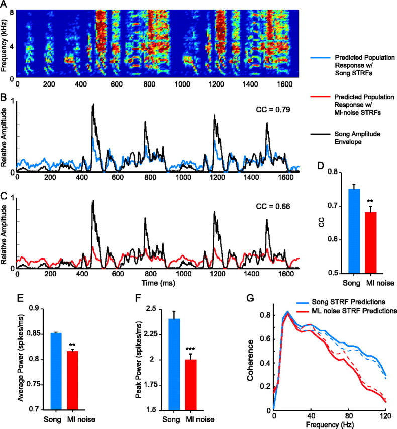
Population synchrony during song processing led to the precise encoding of the temporal patterns in song. A, A spectrogram of song. B, The pPSTH of the predicted response to the sound in A (blue) is plotted with the amplitude envelope of that sound (black). The response follows the temporal pattern; the lines are highly correlated. C, The pPSTH of the response to the sound in A modeled by using ml noise STRFs instead of song STRFs for the same cells (red) is plotted with the amplitude envelope of the sound (black). The lines are less well correlated. D, The mean correlation coefficient (CC) between predicted responses and amplitude envelopes of songs was significantly higher for responses predicted using song STRFs than for those predicted using ml noise STRFs. E, The power of the predicted population response was significantly higher with song STRFs than with ml noise STRFs. F, The mean peak amplitude of responses was also higher for song STRFs. Error bars indicate SE. G, The coherence between predicted population responses and amplitude envelopes was higher for responses predicted by song STRFs than for responses predicted by ml noise STRFs, indicating that song STRF responses encode the temporal patterns of songs with more accuracy than do ml noise STRF responses. The dotted lines show SEs. The two lines differ significantly at 45 Hz (p < 0.05) and above. ***p < 0.001; **p < 0.01.

To assess the role of stimulus-dependent tuning in the population coding of song temporal envelopes, we predicted the responses of individual cells to song using their ml noise STRFs rather than their song STRFs, thereby predicting the “stimulus-independent” population responses to song samples. Results showed that population coding of the temporal patterns of song was significantly less accurate using ml noise STRFs than using song STRFs (Fig. 13). Figure 13C shows the predicted population response to the song sample in A when the tuning to ml noise was used to predict the response (red line). This response follows the amplitude envelope of the song less well than does the response generated by the song STRFs (compare the red and blue lines with the black line). The correlation coefficient between the population response predicted by the ml noise STRFs (red line) and the song amplitude envelope (black line) was 0.66. This effect was true across all songs. The mean (±SE) correlation coefficient between population responses predicted by ml noise STRFs and the song amplitude envelopes was 0.68 ± 0.020, significantly lower than the mean correlation coefficient between song STRF predicted population responses and song amplitude envelopes (Fig. 13D) (p < 0.01). Therefore, if neural tuning did not change between the processing of song and ml noise (i.e., if song STRFs were the same as ml noise STRFs), then the population of MLd neurons would code the temporal patterns of songs with significantly less accuracy than they do.

The predicted population responses to song given by song STRFs and by ml noise STRFs also differed in power. Both the average power, measured using RMS, and the peak power were significantly larger in predicted population responses calculated with song STRFs than with ml noise STRFs. This can be seen in the responses shown in Figure 13 by comparing the blue line in B with the red line in C. The average and peak amplitudes are higher in Figure 13B. Figure 13, E and F, shows the quantification of power for population responses across all songs. The mean (±SE) RMS for predicted responses using song STRFs was 0.85 ± 0.009 spikes/ms (Fig. 13E). The same measure was significantly lower, 0.81 ± 0.016 spikes/ms, for predicted responses to the same songs but using ml noise STRFs (p < 0.01). Similarly, the peak amplitude was significantly higher for responses using song STRFs over responses using ml noise STRFs (Fig. 13F) (p < 0.001). Peak values were 2.4 ± 0.077 and 2.0 ± 0.056 spikes/ms for song STRF and ml noise STRF predicted responses, respectively. The larger average and peak power are attributable to the synchronization achieved by stimulus-dependent receptive field change, which leads to a more constructive summation of responses in the population code. The resulting population code has a higher signal-to-noise ratio than if such changes were absent.

Finally, we determined how well the population responses predicted using song STRFs versus ml noise STRFs matched the temporal patterns of songs at each temporal frequency. For this, we measured the coherence between the song amplitude envelopes and the predicted population responses. Unlike cross-correlation, coherence compares the similarity between two waveforms for individual temporal frequencies. Figure 13G shows that the song STRF responses (blue line) follow the song amplitude envelope better than do the ml noise STRF responses (red line) at modulation frequencies of ≥35 Hz, with significantly different coherences at ≥45 Hz (paired t test; p < 0.05). This difference in coherence between the two predicted responses can be attributed to the increases in temporal precision shown in the STRFs in Figure 7 and quantitatively in Figure 9 and the increase in synchrony across cells illustrated in Figure 11. Synchrony allows the coding of high-frequency temporal modulations by preventing temporal smearing of the population response. Therefore, the changes in linear tuning of individual cells that lead to population synchrony provide a neural mechanism for the encoding of the details of the temporal pattern of a song by a population, potentially providing the information required to discriminate one song from another.

Discussion

We asked whether linear tuning in single auditory neurons differs depending on the sounds that they process by comparing the tuning of single auditory midbrain neurons during the coding of a socially relevant sound, conspecific song, and a generic sound, ml noise. We found that auditory tuning is stimulus dependent in most midbrain neurons; frequency tuning is consistently less selective and temporal tuning is consistently more precise during the coding of song than during the coding of ml noise. This changed linear tuning leads to the synchronization of responses across cells during the coding of song, producing a powerful and temporally precise population response to song. When a model of population tuning was generated based on tuning to ml noise, the responses to song were significantly less precise and lower in power. Therefore, it is possible that the changes in linear auditory tuning that occur during song processing facilitate the neural discrimination of different songs by faithfully reproducing their unique temporal patterns in the neural code. Below, we discuss the evidence for such stimulus-dependent linear tuning in other systems, the potential coding significance of response synchronization among neurons, and the importance of extracting temporal information from auditory signals for perception.

Stimulus-dependent changes in linear tuning

Natural or naturalistic stimuli drive auditory neurons particularly well (Rieke et al., 1995; Escabi et al., 2003; Grace et al., 2003; Hsu et al., 2004). Here, although MLd neurons responded to song and ml noise with the same mean spike rate, response differences between the two stimuli were demonstrated by differences in the spectrotemporal tuning of single neurons. Because different STRFs are needed to describe the responses to different stimulus types, it is clear that the coding is partially nonlinear (Theunissen et al., 2000). Nonlinear coding has also been observed indirectly in cortical neurons, where neural responses to sound can depend on context (for review, see Nelken, 2004). Responses of cat A1 neurons to bird calls have been shown to depend strongly on previous temporal context and background noise (Nelken et al., 1999; Bar-Yosef et al., 2002). Such nonlinear coding would be reflected in the linear coding of a neuron, resulting in STRF differences. Studying these differences may provide insight into the nature of nonlinear tuning.

The stimulus-dependent tuning observed here may be attributable to the following: (1) acoustic differences in the stimuli; song and ml noise drive neurons from the cochlea to the midbrain differently, resulting in different midbrain receptive fields; and/or (2) changes in brain state based on differences such as social meaning between the stimuli; song is associated with arousal and predictably evokes behavioral responses, whereas ml noise is behaviorally arbitrary. Previous studies have described stimulus-dependent differences in receptive field properties in the mammalian auditory midbrain (Escabi and Schreiner, 2002; Escabi et al., 2003), auditory cortex (Valentine and Eggermont, 2004), and primary visual cortex (David et al., 2004; Touryan et al., 2005). Valentine and Eggermont (2004) found that STRFs obtained using simple stimuli were significantly more broadband than those obtained from the same neurons using complex stimuli. David et al. (2004) examined spatiotemporal tuning differences in response to natural versus synthetic visual stimuli. They found, as we did, that STRFs obtained using natural stimuli were twice as good at predicting the actual responses to natural stimuli as the STRFs obtained from the same neurons using synthetic stimuli. Whereas we found that STRFs obtained using song were more spectrally broadband but more temporally narrow, they found that STRFs obtained using natural stimuli had larger inhibitory components and less precise temporal tuning than the STRFs obtained using synthetic gratings. These differences indicate that neurons across sensory systems and organisms may display stimulus-dependent changes in the spectral/spatial and temporal tuning domains, but that the nature of those changes is specific to the system. It also remains to be seen how MLd neurons respond to song stimuli when birds are awake and/or when songs are embedded in typical environmental noise (Nelken et al., 1999; Bar-Yosef et al., 2002).

In songbirds, the presentation of song predictably evokes states of arousal and aggressive or mating-related behaviors (Catchpole and Slater, 1995). By comparison, noise-like sounds are behaviorally neutral. In mammals, experience-dependent changes in linear auditory tuning properties modeled by STRFs have been induced by entraining behavioral significance for certain sounds (Fritz et al., 2003, 2005). It is possible that tuning differences at the level of the midbrain reflect the differential activity of connected brain regions based on the behavioral significance of the sound (i.e., changes in overall brain state). In this way, a neural feedback system whose activity is based on the social importance of a sound could participate in shaping the initial processing of that sound (Engel et al., 2001). Across taxa, the auditory midbrain is known to receive descending inputs (Mello et al., 1998; Winer et al., 1998, 2002; Bajo and Moore, 2005). And the response properties of auditory midbrain neurons have been shown to differ depending on cortical activity (Yan and Suga, 1998; Endepols and Walkowiak, 1999, 2000; Ma and Suga, 2001; Yan and Ehret, 2002).

Stimulus-dependent tuning, population coding, and ensemble synchrony

The stimulus-dependent tuning revealed by responses to song and ml noise resulted in synchronous activity across the neuronal population during the processing of song; receptive fields of individual neurons overlapped substantially more in both the spectral and temporal domains during song processing than during ml noise processing. We found two main effects of the increased synchronicity on the population response. First, the average and peak amplitude of the population responses to song were greater than to ml noise. This may increase the probability of firing in downstream neurons that receive convergent inputs from MLd neurons, thus efficiently propagating the response and potentially maintaining correlated activity in other brain regions (Lestienne, 2001). Second, the response synchrony resulted in a highly temporally precise population response to song. Thus, the neuronal population encoded song as a pattern of fluctuations in instantaneous firing rate over time, creating a neural copy of the unique temporal pattern of a song. The theoretical population response to song that we modeled using the ml noise STRFs showed less synchrony among neurons and therefore had less power and was temporally smeared, eliminating the firing precision required to encode the finer temporal information in song.

Population codes, in which neural activity is summed across a group of neurons, have been successful in predicting perception and motor behavior. Such codes in motor cortex accurately predict the direction of limb movements in primates (Amirikian and Georgopoulos, 1999). In hearing, pooled response patterns have been used to estimate pitch perception (Cariani and Delgutte, 1996). The temporal profile of the population response of the auditory nerve has been shown to be invariant for the same speech utterance under voiced and whispered conditions (Stevens and Wickesberg, 1999). In insects, auditory receptors respond synchronously at the onsets of temporally distinct sounds, producing a neural population response that faithfully mimics the basic temporal pattern of the stimulus (Mason and Faure, 2004). Machens et al. (2001) found that using the population response of grasshoppers’ auditory receptors increased the accuracy of temporal encoding over single responses such that the neural sensitivity to temporal information approached behavioral levels. Similarly, our findings suggest that the auditory midbrain population response could be used to obtain a reliable representation of the amplitude envelope of a song, which is a highly informative stimulus parameter (Woolley et al., 2005).

Population coding as considered by our analyses is only one of many levels of information that downstream neurons may use to code sounds. Auditory tuning in songbird primary forebrain neurons is more complex than that in the midbrain (Woolley et al., 2005). It is possible that differences in the frequency tuning of individual STRFs and nonlinear coding properties are emphasized in regions “higher” than the midbrain, forming receptive fields with complex spectrotemporal properties (Woolley et al., 2005). The activity of subsets of auditory neurons could encode sound parameters other than temporal structure; postsynaptic neurons may use synchronized information from MLd neurons to extract information such as the spectral patterns in songs. How the correlated activity of multiple neurons plays a role in that process has been studied in visual (Salinas and Sejnowski, 2001; Pasupathy and Connor, 2002; Clatworthy et al., 2003; Schnitzer and Meister, 2003; Kenyon et al., 2004; Samonds et al., 2004; van der Togt et al., 2006), olfactory (Friedrich and Stopfer, 2001; Laurent et al., 2001; Friedrich et al., 2004), and auditory neurons (Wang et al., 1995; Gehr et al., 2000; Bodnar et al., 2001; Wotton et al., 2004). Several studies have demonstrated that, when neuronal responses are partially correlated (their receptive fields partially overlap), information about the stimulus is gained from the correlated responses in addition to the independent responses (Dan et al., 1998; deCharms and Merzenich, 1996). When behavioral discrimination of differences in sensory stimuli exceeds the dynamic ranges of single neurons, synchronous activity has been shown to increase the neural sensitivity to stimulus differences (Samonds et al., 2004). The consensus on what information can be gained from the coupled activity of groups of neurons is that considerable increases in sensitivity to stimulus variables such as spatial/spectral and temporal resolution can be achieved.

Coding temporal information and acoustic communication

Our findings suggest that auditory midbrain neurons create a neural representation of the temporal patterns of songs. The importance of temporal patterns for animal communication has been demonstrated in behavioral or psychophysical studies. Speech that is degraded in the spectral domain but with the correct amplitude envelopes is surprisingly understandable (Van Tasell et al., 1987; Shannon et al., 1995). Tamarins produce the same response calls to white noise that is shaped by the amplitude envelopes of their calls as they give to the natural calls (Ghazanfar et al., 2002). Vocal fish and insects also rely heavily on temporal information for recognizing communication signals, (McKibben and Bass, 1998, 2001; Ronacher and Hennig, 2004; Talyn and Dowse, 2004; Jeffery et al., 2005). In songbirds, the temporal patterns of songs are suspected to be important for the discrimination and identification of conspecific and individual songs (Catchpole and Slater, 1995). But little experimental work has addressed this issue. Population coding of temporal patterns that characterize natural communication sounds has been demonstrated in mammals (Wang et al., 1995; Gehr et al., 2000), fish (Bodnar et al., 2001), birds (Woolley et al., 2005), and grasshoppers (Machens et al., 2001). The direct relationship between the perception of communication sounds and how populations of neurons represent such sounds remains to be determined.

References

- Alder TB, Rose GJ (2000). Integration and recovery processes contribute to the temporal selectivity of neurons in the midbrain of the northern leopard frog, Rana pipiens. J Comp Physiol A Neuroethol Sens Neural Behav Physiol 186:923–937. [DOI] [PubMed] [Google Scholar]
- Amirikian B, Georgopoulos AP (1999). Cortical populations and behaviour: Hebb’s thread. Can J Exp Psychol 53:21–34. [DOI] [PubMed] [Google Scholar]
- Bajo VM, Moore DR (2005). Descending projections from the auditory cortex to the inferior colliculus in the gerbil, Meriones unguiculatus. J Comp Neurol 486:101–116. [DOI] [PubMed] [Google Scholar]
- Bar-Yosef O, Rotman Y, Nelken I (2002). Responses of neurons in cat primary auditory cortex to bird chirps: effects of temporal and spectral context. J Neurosci 22:8619–8632. [DOI] [PMC free article] [PubMed] [Google Scholar]
- Bass AH, McKibben JR (2003). Neural mechanisms and behaviors for acoustic communication in teleost fish. Prog Neurobiol 69:1–26. [DOI] [PubMed] [Google Scholar]
- Bodnar DA, Holub AD, Land BR, Skovira J, Bass AH (2001). Temporal population code of concurrent vocal signals in the auditory midbrain. J Comp Physiol A Neuroethol Sens Neural Behav Physiol 187:865–873. [DOI] [PubMed] [Google Scholar]
- Cariani PA, Delgutte B (1996). Neural correlates of the pitch of complex tones. I. Pitch and pitch salience. J Neurophysiol 76:1698–1716. [DOI] [PubMed] [Google Scholar]
- Casseday JH, Ehrlich D, Covey E (1994). Neural tuning for sound duration: role of inhibitory mechanisms in the inferior colliculus. Science 264:847–850. [DOI] [PubMed] [Google Scholar]
- Catchpole CK, Slater PJB (1995). In: Bird song Cambridge, UK: Cambridge UP.
- Chi T, Gao Y, Guyton MC, Ru P, Shamma S (1999). Spectro-temporal modulation transfer functions and speech intelligibility. J Acoust Soc Am 106:2719–2732. [DOI] [PubMed] [Google Scholar]
- Clatworthy PL, Chirimuuta M, Lauritzen JS, Tolhurst DJ (2003). Coding of the contrasts in natural images by populations of neurons in primary visual cortex (V1). Vision Res 43:1983–2001. [DOI] [PubMed] [Google Scholar]
- Covey E, Casseday JH (1999). Timing in the auditory system of the bat. Annu Rev Physiol 61:457–476. [DOI] [PubMed] [Google Scholar]
- Dan Y, Alonso JM, Usrey WM, Reid RC (1998). Coding of visual information by precisely correlated spikes in the lateral geniculate nucleus. Nat Neurosci 1:501–507. [DOI] [PubMed] [Google Scholar]
- David SV, Vinje WE, Gallant JL (2004). Natural stimulus statistics alter the receptive field structure of v1 neurons. J Neurosci 24:6991–7006. [DOI] [PMC free article] [PubMed] [Google Scholar]
- Dear SP, Suga N (1995). Delay-tuned neurons in the midbrain of the big brown bat. J Neurophysiol 73:1084–1100. [DOI] [PubMed] [Google Scholar]
- de Boer R, Kuyper P (1968). Triggered correlation. IEEE Trans Biomed Eng 15:169–179. [DOI] [PubMed] [Google Scholar]
- deCharms RC, Merzenich MM (1996). Primary cortical representation of sounds by the coordination of action-potential timing. Nature 381:610–613. [DOI] [PubMed] [Google Scholar]
- Endepols H, Walkowiak W (1999). Influence of descending forebrain projections on processing of acoustic signals and audiomotor integration in the anuran midbrain. Eur J Morphol 37:182–184. [DOI] [PubMed] [Google Scholar]
- Endepols H, Walkowiak W (2000). Integration of ascending and descending inputs in the auditory midbrain of anurans. J Comp Physiol A Neuroethol Sens Neural Behav Physiol 186:1119–1133. [DOI] [PubMed] [Google Scholar]
- Engel AK, Fries P, Singer W (2001). Dynamic predictions: oscillations and synchrony in top-down processing. Nat Rev Neurosci 2:704–716. [DOI] [PubMed] [Google Scholar]
- Escabi MA, Schreiner CE (2002). Nonlinear spectrotemporal sound analysis by neurons in the auditory midbrain. J Neurosci 22:4114–4131. [DOI] [PMC free article] [PubMed] [Google Scholar]
- Escabi MA, Miller LM, Read HL, Schreiner CE (2003). Naturalistic auditory contrast improves spectrotemporal coding in the cat inferior colliculus. J Neurosci 23:11489–11504. [DOI] [PMC free article] [PubMed] [Google Scholar]
- Friedrich RW, Stopfer M (2001). Recent dynamics in olfactory population coding. Curr Opin Neurobiol 11:468–474. [DOI] [PubMed] [Google Scholar]
- Friedrich RW, Habermann CJ, Laurent G (2004). Multiplexing using synchrony in the zebrafish olfactory bulb. Nat Neurosci 7:862–871. [DOI] [PubMed] [Google Scholar]
- Fritz J, Shamma S, Elhilali M, Klein D (2003). Rapid task-related plasticity of spectrotemporal receptive fields in primary auditory cortex. Nat Neurosci 6:1216–1223. [DOI] [PubMed] [Google Scholar]
- Fritz JB, Elhilali M, Shamma SA (2005). Differential dynamic plasticity of A1 receptive fields during multiple spectral tasks. J Neurosci 25:7623–7635. [DOI] [PMC free article] [PubMed] [Google Scholar]
- Gehr DD, Komiya H, Eggermont JJ (2000). Neuronal responses in cat primary auditory cortex to natural and altered species-specific calls. Hear Res 150:27–42. [DOI] [PubMed] [Google Scholar]
- Ghazanfar AA, Smith-Rohrberg D, Pollen AA, Hauser MD (2002). Temporal cues in the antiphonal long-calling behaviour of cottontop tamarins. Anim Behav 64:427–438. [Google Scholar]
- Grace JA, Amin N, Singh NC, Theunissen FE (2003). Selectivity for conspecific song in the zebra finch auditory forebrain. J Neurophysiol 89:472–487. [DOI] [PubMed] [Google Scholar]
- Hsu A, Woolley SM, Fremouw TE, Theunissen FE (2004). Modulation power and phase spectrum of natural sounds enhance neural encoding performed by single auditory neurons. J Neurosci 24:9201–9211. [DOI] [PMC free article] [PubMed] [Google Scholar]
- Jeffery J, Navia B, Atkins G, Stout J (2005). Selective processing of calling songs by auditory interneurons in the female cricket, Gryllus pennsylvanicus: possible roles in behavior. J Exp Zoolog A Comp Exp Biol 303:377–392. [DOI] [PubMed] [Google Scholar]
- Kelley DB (2004). Vocal communication in frogs. Curr Opin Neurobiol 14:751–757. [DOI] [PubMed] [Google Scholar]
- Kenyon GT, Theiler J, George JS, Travis BJ, Marshak DW (2004). Correlated firing improves stimulus discrimination in a retinal model. Neural Comput 16:2261–2291. [DOI] [PubMed] [Google Scholar]
- Laurent G, Stopfer M, Friedrich RW, Rabinovich MI, Volkovskii A, Abarbanel HD (2001). Odor encoding as an active, dynamical process: experiments, computation, and theory. Annu Rev Neurosci 24:263–297. [DOI] [PubMed] [Google Scholar]
- Lestienne R (2001). Spike timing, synchronization and information processing on the sensory side of the central nervous system. Prog Neurobiol 65:545–591. [DOI] [PubMed] [Google Scholar]
- Ma X, Suga N (2001). Corticofugal modulation of duration-tuned neurons in the midbrain auditory nucleus in bats. Proc Natl Acad Sci USA 98:14060–14065. [DOI] [PMC free article] [PubMed] [Google Scholar]
- Machens CK, Stemmler MB, Prinz P, Krahe R, Ronacher B, Herz AV (2001). Representation of acoustic communication signals by insect auditory receptor neurons. J Neurosci 21:3215–3227. [DOI] [PMC free article] [PubMed] [Google Scholar]
- Marsat G, Pollack GS (2005). Effect of the temporal pattern of contralateral inhibition on sound localization cues. J Neurosci 25:6137–6144. [DOI] [PMC free article] [PubMed] [Google Scholar]
- Mason AC, Faure PA (2004). The physiology of insect auditory afferents. Microsc Res Tech 63:338–350. [DOI] [PubMed] [Google Scholar]
- McAnally KI, Stein JF (1996). Auditory temporal coding in dyslexia. Proc Biol Sci 263: pp. 961–965. [DOI] [PubMed] [Google Scholar]
- McKibben JR, Bass AH (1998). Behavioral assessment of acoustic parameters relevant to signal recognition and preference in a vocal fish. J Acoust Soc Am 104:3520–3533. [DOI] [PubMed] [Google Scholar]
- McKibben JR, Bass AH (2001). Effects of temporal envelope modulation on acoustic signal recognition in a vocal fish, the plainfin midshipman. J Acoust Soc Am 109:2934–2943. [DOI] [PubMed] [Google Scholar]
- Mello CV, Vates GE, Okuhata S, Nottebohm F (1998). Descending auditory pathways in the adult male zebra finch (Taeniopygia guttata). J Comp Neurol 395:137–160. [PubMed] [Google Scholar]
- Mittmann DH, Wenstrup JJ (1995). Combination-sensitive neurons in the inferior colliculus. Hear Res 90:185–191. [DOI] [PubMed] [Google Scholar]
- Nelken I (2004). Processing of complex stimuli and natural scenes in the auditory cortex. Curr Opin Neurobiol 14:474–480. [DOI] [PubMed] [Google Scholar]
- Nelken I, Rotman Y, Bar-Yosef O (1999). Responses of auditory-cortex neurons to structural features of natural sounds. Nature 397:154–157. [DOI] [PubMed] [Google Scholar]
- Pasupathy A, Connor CE (2002). Population coding of shape in area V4. Nat Neurosci 5:1332–1338. [DOI] [PubMed] [Google Scholar]
- Pollak GD, Bodenhamer RD (1981). Specialized characteristics of single units in inferior colliculus of mustache bat: frequency representation, tuning, and discharge patterns. J Neurophysiol 46:605–620. [DOI] [PubMed] [Google Scholar]
- Rieke F, Bodnar DA, Bialek W (1995). Naturalistic stimuli increase the rate and efficiency of information transmission by primary auditory afferents. Proc Biol Sci 262: pp. 259–265. [DOI] [PubMed] [Google Scholar]
- Ringach DL, Sapiro G, Shapley R (1997). A subspace reverse-correlation technique for the study of visual neurons. Vision Res 37:2455–2464. [DOI] [PubMed] [Google Scholar]
- Ronacher B, Hennig RM (2004). Neuronal adaptation improves the recognition of temporal patterns in a grasshopper. J Comp Physiol A Neuroethol Sens Neural Behav Physiol 190:311–319. [DOI] [PubMed] [Google Scholar]
- Ronacher B, Franz A, Wohlgemuth S, Hennig RM (2004). Variability of spike trains and the processing of temporal patterns of acoustic signals—problems, constraints, and solutions. J Comp Physiol A Neuroethol Sens Neural Behav Physiol 190:257–277. [DOI] [PubMed] [Google Scholar]
- Rose GJ, Capranica RR (1983). Temporal selectivity in the central auditory system of the leopard frog. Science 219:1087–1089. [DOI] [PubMed] [Google Scholar]
- Rose GJ, Capranica RR (1985). Sensitivity to amplitude modulated sounds in the anuran auditory nervous system. J Neurophysiol 53:446–465. [DOI] [PubMed] [Google Scholar]
- Sahani M, Dayan P (2003). Doubly distributional population codes: simultaneous representation of uncertainty and multiplicity. Neural Comput 15:2255–2279. [DOI] [PubMed] [Google Scholar]
- Salinas E, Sejnowski TJ (2001). Correlated neuronal activity and the flow of neural information. Nat Rev Neurosci 2:539–550. [DOI] [PMC free article] [PubMed] [Google Scholar]
- Samonds JM, Allison JD, Brown HA, Bonds AB (2004). Cooperative synchronized assemblies enhance orientation discrimination. Proc Natl Acad Sci USA 101:6722–6727. [DOI] [PMC free article] [PubMed] [Google Scholar]
- Schnitzer MJ, Meister M (2003). Multineuronal firing patterns in the signal from eye to brain. Neuron 37:499–511. [DOI] [PubMed] [Google Scholar]
- Shannon RV, Zeng FG, Kamath V, Wygonski J, Ekelid M (1995). Speech recognition with primarily temporal cues. Science 270:303–304. [DOI] [PubMed] [Google Scholar]
- Singh NC, Theunissen FE (2003). Modulation spectra of natural sounds and ethological theories of auditory processing. J Acoust Soc Am 114:3394–3411. [DOI] [PubMed] [Google Scholar]
- Stevens HE, Wickesberg RE (1999). Ensemble responses of the auditory nerve to normal and whispered stop consonants. Hear Res 131:47–62. [DOI] [PubMed] [Google Scholar]
- Suga N (1989). Principles of auditory information-processing derived from neuroethology. J Exp Biol 146:277–286. [DOI] [PubMed] [Google Scholar]
- Tallal P, Miller S, Fitch RH (1993). Neurobiological basis of speech: a case for the preeminence of temporal processing. Ann NY Acad Sci 682:27–47. [DOI] [PubMed] [Google Scholar]
- Talyn BC, Dowse HB (2004). The role of courtship song in sexual selection and species recognition by female Drosophila melanogaster. Anim Behav 68:1165–1180. [Google Scholar]
- Theunissen FE, Sen K, Doupe AJ (2000). Spectral-temporal receptive fields of nonlinear auditory neurons obtained using natural sounds. J Neurosci 20:2315–2331. [DOI] [PMC free article] [PubMed] [Google Scholar]
- Theunissen FE, David SV, Singh NC, Hsu A, Vinje WE, Gallant JL (2001). Estimating spatio-temporal receptive fields of auditory and visual neurons from their responses to natural stimuli. Network 12:289–316. [PubMed] [Google Scholar]
- Theunissen FE, Woolley SM, Hsu A, Fremouw T (2004). Methods for the analysis of auditory processing in the brain. Ann NY Acad Sci 1016:187–207. [DOI] [PubMed] [Google Scholar]
- Touryan J, Felsen G, Dan Y (2005). Spatial structure of complex cell receptive fields measured with natural images. Neuron 45:781–791. [DOI] [PubMed] [Google Scholar]
- Valentine PA, Eggermont JJ (2004). Stimulus dependence of spectro-temporal receptive fields in cat primary auditory cortex. Hear Res 196:119–133. [DOI] [PubMed] [Google Scholar]
- van der Togt C, Kalitzin S, Spekreijse H, Lamme VA, Super H (2006). Synchrony dynamics in monkey V1 predict success in visual detection. Cereb Cortex 16:136–148. [DOI] [PubMed] [Google Scholar]
- Van Tasell DJ, Soli SD, Kirby VM, Widin GP (1987). Speech waveform envelope cues for consonant recognition. J Acoust Soc Am 82:1152–1161. [DOI] [PubMed] [Google Scholar]
- Wang X, Merzenich MM, Beitel R, Schreiner CE (1995). Representation of a species-specific vocalization in the primary auditory cortex of the common marmoset: temporal and spectral characteristics. J Neurophysiol 74:2685–2706. [DOI] [PubMed] [Google Scholar]
- Winer JA, Larue DT, Diehl JJ, Hefti BJ (1998). Auditory cortical projections to the cat inferior colliculus. J Comp Neurol 400:147–174. [PubMed] [Google Scholar]
- Winer JA, Chernock ML, Larue DT, Cheung SW (2002). Descending projections to the inferior colliculus from the posterior thalamus and the auditory cortex in rat, cat, and monkey. Hear Res 168:181–195. [DOI] [PubMed] [Google Scholar]
- Woolley SM, Casseday JH (2004). Response properties of single neurons in the zebra finch auditory midbrain: response patterns, frequency coding, intensity coding, and spike latencies. J Neurophysiol 91:136–151. [DOI] [PubMed] [Google Scholar]
- Woolley SM, Casseday JH (2005). Processing of modulated sounds in the zebra finch auditory midbrain: responses to noise, frequency sweeps, and sinusoidal amplitude modulations. J Neurophysiol 94:1143–1157. [DOI] [PubMed] [Google Scholar]
- Woolley SM, Rubel EW (1999). High-frequency auditory feedback is not required for adult song maintenance in Bengalese finches. J Neurosci 19:358–371. [DOI] [PMC free article] [PubMed] [Google Scholar]
- Woolley SM, Fremouw T, Hsu A, Theunissen FE (2005). Tuning for spectro-temporal modulations as a mechanism for discrimination of natural sounds. Nat Neurosci 8:1371–1379. [DOI] [PubMed] [Google Scholar]
- Wotton JM, Ferragamo MJ, Sanderson MI (2004). The emergence of temporal hyperacuity from widely tuned cell populations. Network 15:159–177. [PubMed] [Google Scholar]
- Wright BA, Lombardino LJ, King WM, Puranik CS, Leonard CM, Merzenich MM (1997). Deficits in auditory temporal and spectral resolution in language-impaired children. Nature 387:176–178. [DOI] [PubMed] [Google Scholar]
- Yan J, Ehret G (2002). Corticofugal modulation of midbrain sound processing in the house mouse. Eur J Neurosci 16:119–128. [DOI] [PubMed] [Google Scholar]
- Yan W, Suga N (1998). Corticofugal modulation of the midbrain frequency map in the bat auditory system. Nat Neurosci 1:54–58. [DOI] [PubMed] [Google Scholar]