Local Homogeneity of Cell Cycle Length in Developing Mouse Cortex

Abstract

We have measured the amount of variation in the length of the cell cycle for cells in the pseudostratified ventricular epithelium (PVE) of the developing cortex of mice on embryonic day 14. Our measurements were made in three cortical regions (i.e., the neocortex, archicortex, and periarchicortex) using three different methods: the cumulative labeling method (CLM), the percent labeled mitoses (PLM) method, and a comparison of the time needed for the PLM to ascend from 0 to 100% with the time needed for the PLM to descend from 100 to 0%. These 3 different techniques provide different perspectives on the cytokinetic parameters. Theoretically, CLM gives an estimate for a maximum value of the total length of the cell cycle (T_C), whereas PLM gives an estimate of a minimum value of T_C. The difference between these two estimates indicates that the range for T_Cis ±1% of the mean T_C for periarchicortex, ±7% for neocortex, and ±8% for archicortex. This was confirmed by a lengthening of the PLM descent time in comparison with its ascent time. The sharpness of the transitions and the flatness of the plateau of the PLM curves indicate that 99% of the proliferating cells are within this narrow estimated range for T_C; hence, only ∼1% deviate outside of a relatively restricted range from the average T_C of the population. In the context of the possible existence within the cortical PVE of two populations with markedly dissimilar cell cycle kinetics from the mean, one such population must comprise ∼99% of the total population, and the other, if it exists, is only ∼1% of the total. This seems to be true for all three cortical regions. The narrow range of T_C indicates a homogeneity in the cell cycle length for proliferating cells in three different cortical regions, despite the fact that progenitor cells of different lineages may be present. It further predicts the existence of almost synchronous interkinetic nuclear movements of the proliferating cells in the ventricular zone during early development of the cerebral cortex.

In the mammalian cortex, most neuronogenesis occurs in a pseudostratified ventricular epithelium (PVE) that occupies the ventricular zone adjacent to the lateral ventricle. Within the PVE, proliferating cells undergo interkinetic nuclear migration such that the position of the nucleus correlates with the phase of the cell cycle. DNA synthesis or S phase occurs in the outer half of the ventricular zone, and mitosis occurs at the ventricular surface (Angevine and Sidman, 1961; Rakic, 1972; Caviness and Sidman, 1973;Takahashi et al., 1995a). Thus, during a single cell cycle, the nucleus of a proliferating cell moves from the ventricular surface outward during G₁ and returns to the ventricular surface during S and G₂. The time required for a single cell cycle has been measured in previous studies of cell cycle kinetics that have exploited both the percent labeled mitoses (PLM) method (Hoshino et al., 1973;Cai et al., 1993; Takahashi et al., 1993; Reznikov and van der Kooy, 1995) and also the cumulative labeling method (CLM; Waechter and Jaensch, 1972; Miller and Nowakowski, 1988; Nowakowski et al., 1989;Cai et al., 1993; Takahashi et al., 1992, 1993, 1995a; Reznikov and van der Kooy, 1995). Taken together, these studies have measured the lengths of each cell cycle during the neuronogenetic period and demonstrated that the cell cycle lengthens as development proceeds. Relatively little attention, however, has been paid to the variation of cell cycle time at any particular stage of development. In this respect, using cumulative labeling with 5-bromo-2′-deoxyuridine (BUdR),Nowakowski et al. (1989) and Takahashi et al. (1993) found that the labeling index (LI) increases linearly until all proliferating cells are labeled. This linearity indicates that, in terms of the length of the cell cycle (T_C) and the length of the S phase (T_S), the cells of the PVE constitute a single population and move through the cell cycle at approximately the same rate. Specifically, it has been estimated from these results that 80–90% of the proliferating cells have cytokinetic parameters within ∼10% of the mean (Nowakowski et al., 1989). Thus, it remains possible that as many as 10–20% of the PVE cells have significantly different cytokinetic parameters. To investigate this possibility, we have measured the range of times (i.e., the maximum and minimum time needed for cells to complete a single cell cycle) and the variation in time required for a labeled cohort of cells to enter versus leave M phase, and estimated the purity of the proliferating population in terms of T_C.

The present analysis is focused on the PVE of three different subdivisions of the E14 mouse cortex: the neocortex, archicortex, and periarchicortex (Fig. 1). These three subdivisions differ clearly in their proliferative population. In the archicortex, there is only a single proliferative population (Nowakowski and Rakic, 1981), the PVE. In the neocortex and periarchicortex, in addition to the PVE, there is a secondary proliferative population (SPP), which is believed to be the source of most neuroglial cells (Takahashi et al., 1995b). Because there is no SPP in the archicortex, both neuronal and glial lineages presumably arise from the PVE (Nowakowski and Rakic, 1981). In addition, the PVE of neocortex probably contains not only the progenitors of neurons but also the progenitors of proliferative radial glial cells and perhaps other glial cells (Levitt et al., 1981;Nowakowski and Rakic, 1981; Caviness, 1982; Misson et al., 1988a,b). Thus, it is likely that there are progenitor cells of different lineages (e.g., neuronal and glial) in the PVE and that their proportions differ in various cortical subdivisions. Thus, the results of the present study address the general issue of whether the proliferative populations giving rise to different lineages in the PVE have different or similar cell cycle parameters.

Fig. 1.

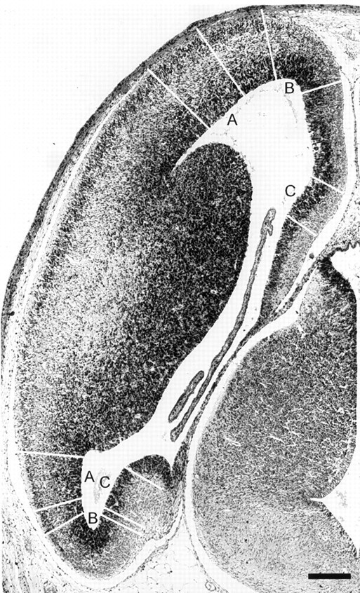
A section through a cerebral hemisphere of the E14 mouse to illustrate the location of the cortical subdivisions analyzed. The three areas can be distinguished by their unique structure and their location and are indicated by white lines spanning the pallium and by letters in the lateral ventricles. The neocortical region analyzed was in the lateral wall (A); the archicortical region analyzed was in the hippocampal anlage in the medial wall (C); and the periarchicortical region analyzed occupied the curve near the rostral or caudal tip of the brain (B). On this approximately horizontal section, the areas analyzed are sectioned twice, once in the rostral portion of the cerebrum (top) and once in the caudal portion of the cerebrum (bottom). The areas selected for analysis always included all three cortical areas on a single section and subtended 200 μm along the ventricular surface. Scale bar, 200 μm.

MATERIALS AND METHODS

Animals. Timed-pregnant CD-1 mice were purchased from Charles River Laboratories (Wilmington, MA) and maintained on a 12 hr/12 hr (7:00 A.M. to 7:00 P.M.) light/dark schedule from the time of arrival until the time of the experiment. Pregnancies were timed from the day on which a vaginal plug was detected, designated as E0. All experiments were initiated at 8:00 AM on E14.

Cumulative labeling with BUdR. The CLM with BUdR has been described in detail elsewhere (Nowakowski et al., 1989). On E14, dams received i.p. injections of BUdR (50 μg/gm body weight in 0.9% NaCl, 0.007 N NaOH) at 2 hr intervals over a total period of 12 hr, beginning at 8:00 A.M. Thirty min after each of the BUdR injections, selected dams were deeply anesthetized with 4% chloral hydrate, and the fetuses were removed by hysterotomy and fixed by immersion in 4% phosphate buffered paraformaldehyde, pH 7.4. A total of 18 litters were collected at a total of 7 time points.

PLM method. On E14, dams received a single i.p. injection of BUdR at 8:00 AM. Litters were harvested as described above at intervals ranging from 30 min to 2 hr over a total period of 17.5 hr. A total of 35 litters at 25 time points were collected. Note that at certain critical time points, such as near the beginning and end of the rise time and fall time of the mitotic labeling index (MLI), the interval between the collection times was decreased, and the number of litters used per time point was increased to provide optimal temporal resolution. As a result, the PLM data have a resolution of ∼0.5 hr.

Histology. All embryos were staged (Theiler, 1972) immediately after hysterotomy; specimens younger or older than E14 were excluded from this analysis. Subsequently, tissue was processed for BUdR immunohistochemistry according to a modification of Nowakowski et al. (1989). The dorsal skull was removed, and the brains were post-fixed in situ overnight, washed, dehydrated through a graded ethanol series, cleared, and embedded in paraplast. The brains were sectioned serially at 4 μm in a plane approximating a horizontal section and mounted on glass slides pretreated with 3-aminopropyl-triethoxysilane. Slides containing both rostral and caudal portions of the archicortex were deparaffinized, treated with 0.1% trypsin to disrupt the cross linkage of tissue proteins, and with 2 N HCl to produce single-stranded DNA, then processed for immunohistochemical visualization of BUdR using an antibody against single-stranded DNA (Becton-Dickinson 1:75), a Vectastain Elite ABC kit (Mouse IgG), and DAB with cobalt–nickel color intensification; slides were counterstained with 1% basic fuchsin.

Nomenclature. The standard abbreviations for the lengths of the four phases of the cell cycle, i.e., G₁, S, G₂, and M were used. When specific reference is made to the length of one of the phases it is used as a subscript for T (representing “time”); thus, T_G1 is the length of G₁, T_S is the length of S, etc. For consistency, the abbreviation T_C was used to refer to the length of the entire cell cycle. A table of these standard abbreviations was previously published (Nowakowski et al., 1989).

Analysis. Two to six fetuses from each litter were included in the analysis. For each specimen, a sector of 200 μm along the ventricular surface was delineated in each of the three cortical areas (neocortex, archicortex, and “periarchicortex”, see Fig. 1) in three to five nonadjacent sections. Archicortex was recognized by its position on the medial wall of the hemisphere and its lack of a subventricular zone; neocortex was recognized by its position on the lateral wall of the hemisphere and the presence of a small subventricular zone. Periarchicortex was arbitrarily defined as occupying the perimeter of the archicortex, and in this study probably included both incipient entorhinal and incipient cingulate cortex. For all three cortical areas, data from both rostral and caudal extents of the cortex were pooled to obtain enough labeled mitotic figures to perform the PLM method.

CLM. For each of the seven time points, a minimum of eight fetuses per time point were processed. However, data from some fetuses were not available as a result of technical artifacts (i.e., wrong plane of section, failure in immunohistochemical processing, etc.). Data were analyzed from all fetuses not excluded for technical reasons and were from a total of 18 litters containing 42 fetuses. At each time point, the data analyzed were obtained from at least four fetuses from at least two different litters. For each section, the positions of BUdR-labeled and unlabeled nuclei in each 200 μm sector were recorded on drawings made with the aid of a camera lucida, and the numbers of each type of nuclei were counted. The design and interpretation of the CLM has been described in detail previously (Nowakowski et al., 1989). In brief, cells of the PVE in S phase are labeled cumulatively by repeated exposures to BUdR until all proliferating cells have been labeled. The LI (i.e., the ratio of labeled nuclei to total nuclei) at each time point is plotted as a function of time after the first injection. The growth fraction (GF, i.e., the ratio of proliferating cells to the total number of cells in the population) and the values of T_C and T_S are then calculated as described previously (Nowakowski et al., 1989; Takahashi et al., 1992), using a nonlinear least squares fit that considers all of the data points.

PLM method. A total of 35 litters at 25 time points were collected. At least 2 fetuses were analyzed for each of the 25 time points. Because of technical limitations, specimens could be collected and processed for only ∼7–8 time points per experimental group; therefore, the data were collected in four experimental groups. Each experimental group was treated identically, except that the sacrifice times for the litters were varied for each experimental group so that the critical rise and fall times of the MLI plot (Fig. 5) would contain data from at least two and preferably three different time points. For each specimen, all labeled and unlabeled mitotic figures (Fig.2), along the ventricular surface in each of the 200 μm sectors, were counted in both right and left hemispheres of each brain. Mitotic figures of endothelial cells were excluded. A total of 10,219 mitotic figures in 66 fetuses were analyzed.

Fig. 5.

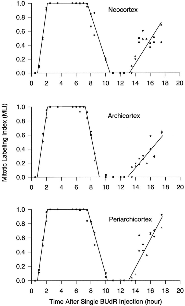
Graphs of the MLI of the developing cortex of the E14 mouse after a single injection of BUdR. MLI was calculated for each section and averaged for each fetus and then averaged for each litter; data for each litter (2–4 fetuses) were then plotted as a function of time after the single BUdR injection. The length of each phase of the cell cycle was determined from this plot as shown. Data points in the three different shapes (i.e., square,circle, triangle, and inverted triangle) at single time points represent data from different litters belonging to different experimental groups (see Materials and Methods). Note that in some cases the plotted data points from the different experimental groups fall exactly on top of one another and, hence, obscure the existence of the different shapes; this most frequently occurs for data across the 100% plateau. The location and length of the rise and fall phases were obtained using a linear least-squares fit to the data points that are clearly on the rising or falling phase, respectively. The values of all cell cycle parameters were derived from these data according to the methods illustrated in the graph in the bottom left corner in Figure 3 and are summarized in Table 1. A, Neocortex; B, archicortex; C, periarchicortex.

Fig. 2.

Photomicrographs of 4-μm-thick horizontal sections through the neocortical PVE in the lateral region of the cerebral wall of E14 mice after in utero exposure to a single BUdR injection. A, Animal killed 1.0 hr after injection, before the labeled cohort of cells has entered M phase.B, Animal killed 5.5 hr after injection, well after the labeled cohort entered M phase. C, Animal killed 10.5 hr after injection, when the labeled cohort had exited M phase. Unlabeled (arrows) and labeled (arrowheads) mitotic figures are located along the margin of the lateral ventricle. The tissue was processed for BUdR immunohistochemistry and lightly counterstained with basic fuchsin. V, Lateral ventricle. Scale bar, 20 μm.

A single injection of BUdR labels a cohort of cells that are in S phase at the time of the injection. The cells of this cohort remain labeled as they progress through the cell cycle, and during M phase they are easily recognized as labeled mitotic figures. The MLI (i.e., the ratio of labeled mitotic figures to total mitotic figures) was calculated for each section and averaged for each fetus. Data for each fetus were then plotted, using a least squares fit that considers all of the data points, as a function of time after the BUdR injection, and the duration of all phases of the cell cycle were determined from this plot (Fig. 3) as follows: the time between injection of BUdR and the appearance of the first labeled mitotic figure is a measurement of T_G2. An estimate of this time was determined from the X-intercept of a linear least squares fit to the data points comprising the rising phase of the plots shown in Figure 5. The time required for the leading cells of the labeled cohort to enter M phase and MLI to reach 100% is T_G2+M. An estimate of this time was obtained from the 100% intercept of a linear least squares fit to the data lying on the ascending phase of the plots in Figure 5. MLI stays at 100% for a time approximately equal to T_S–T_Mand then decreases back to 0%. When the leading cells of this same cohort reenter M phase, a second rise of MLI begins. T_C is obtained by measuring the time interval between two corresponding points in sequential cell cycles (Kauffman, 1968; Hoshino et al., 1973;Steel, 1977; Reznikov and van der Kooy, 1995). T_G1 is obtained by subtraction, T_G1 = T_C − (T_S + T_G2 + T_M).

Fig. 3.

Experimental design for the PLM method. The progression of cells through the cell cycle is depicted in both parts of the figures. The numbers 0–6 correspond in the two graphs. 0, At the initiation of the experiment, a single injection of BUdR labels a cohort of cells that are in S phase at the time of the injection (heavy line). 1, Labeled cohort progresses through the cell cycle, and soon after the lead cell enters M phase the first labeled mitotic figure appears. The time between injection of the BUdR and the appearance of the first labeled mitotic figure is approximately the length of G₂.2, When the lead labeled cell reaches the end of M phase, all metaphase cells will be labeled, at which time the MLI will reach 100%. The time of injection to the time when MLI reaches 100% is approximately equal to the duration of G₂ + M.3, As the cohort continues to progress through the cell cycle, the MLI will remain at 100% until soon after the first unlabeled cell has entered M. At this time, unlabeled metaphase cells will begin to appear. 4, When the trailing cell of the labeled cohort has exited M, MLI once again is 0%. 5, When the labeled lead cell reenters M phase, a new rise time of MLI begins. The interval between corresponding points in two successive cell cycles (e.g., 1 and 5) provides a measure of T_C. All other cytokinetic parameters (i.e., T_S, T_G1, T_M, and T_G2) can be obtained by calculation.

Comparison of the rise time and fall time of the MLI. The cell cycle length increases as development proceeds. To determine the variation of T_C within a single cell cycle, we compared the time needed for the MLI to rise from 0 to 100% with the time needed for the MLI to fall from 100 to 0%. The difference between the fall time and rise time is a measurement of the variability of lengthening within a single cell cycle because of the mixing of fast cycling unlabeled cells with slowly cycling labeled cells.

RESULTS

The cell cycle parameters in subdivisions of developing cortex of E14 mouse as measured by both the CLM (Fig. 4) and the PLM method (Fig. 5) are summarized in Table1.

Fig. 4.

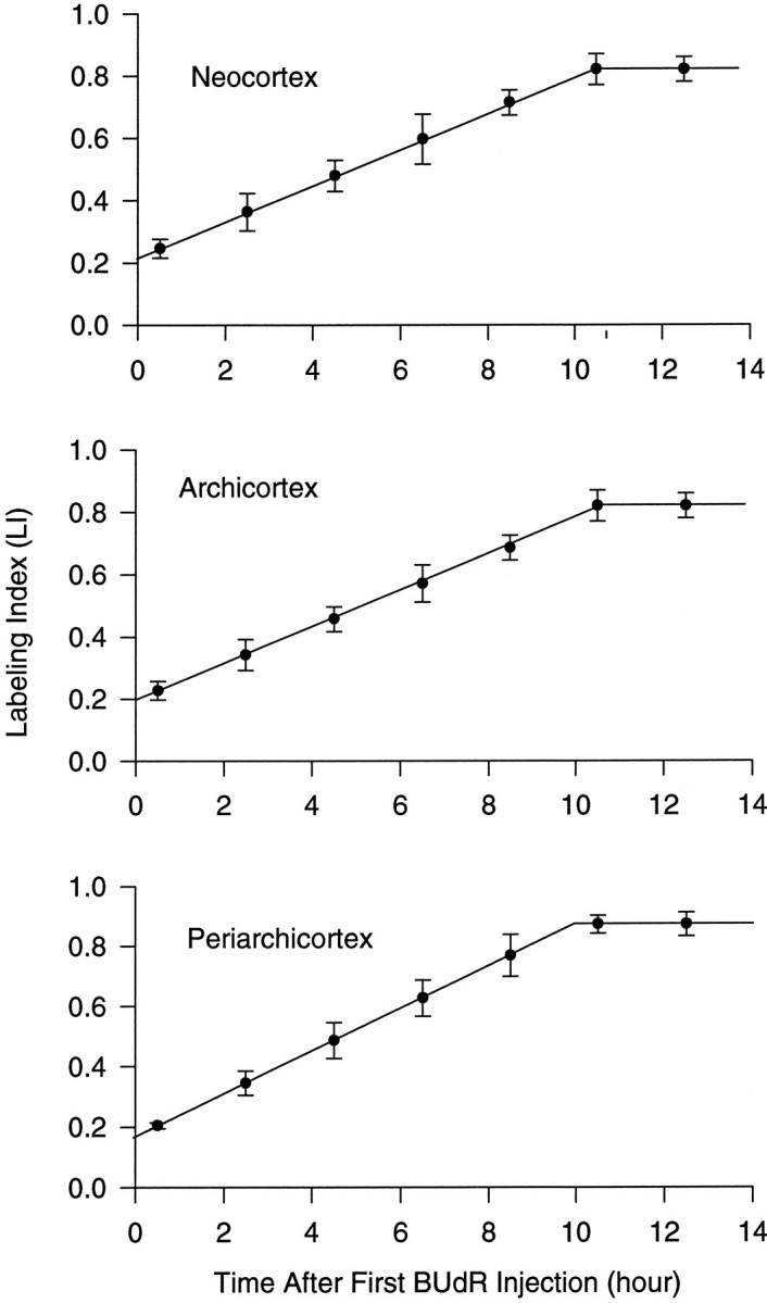
Graphs of LI of the developing cortex of the E14 mouse using the BUdR CLM. LI increases linearly until all proliferating cells (GF) have been labeled; labeling of GF occurs at a time equal to T_C − T_S. The labeling index at they-intercept corresponds to T_S/T_C × GF. They-intercept and inflection of the curve are extrapolated from a least-squares fit slope from all data points (for a complete discussion, see Nowakowski et al., 1989). The values of all cell cycle parameters derived from these data are summarized in Table 1.A, Neocortex; B, archicortex;C, periarchicortex.

Table 1.

Cytokinetic parameters of the PVE in E14 mouse cortex as measured by CLM and PLM method

Cortical subdivision	CLM			PLM method					Δ TC (hr)	% of mean TC
	GF	TC (hr)	TS (hr)	TC (hr)	TS (hr)	TM (hr)	TG1 (hr)	TG2 (hr)
Neocortex	0.8	14.0	3.7	12.3	6.5	1.2	3.7	0.9	1.7	13.3 (±6.7)
Archicortex	0.8	14.3	3.5	12.1	6.6	1.4	3.4	0.8	2.2	16.7 (±8.3)
Periarchicortex	0.9	12.4	2.4	12.2	6.5	1.3	3.6	0.8	0.2	1.5 (±0.7)

The parameters in columns 2–4 are from the data plotted in Figure 4; the parameters in columns 5–9 are from the data plotted in Figure 5; the estimated range of T_C [i.e., the calculated difference in the two estimates of T_C (column 5 − column 3)] is shown in column 10; and the % of the range (and the estimated variation) are listed in the last column.

Cell cycle parameters as determined by the CLM

In each of the three cortical subdivisions analyzed, LI plotted as a function of time increased linearly until the GF was labeled (Fig.4), after which LI no longer increased. At E14, GF was 0.82 in the neocortex, 0.82 in the archicortex, and 0.87 in the periarchicortex. T_C and T_S were calculated from the graphs based on the following two relationships: (1) the time required to label the GF, i.e., the inflection point of the curve, is equal to T_C- T_S; and (2) the y-intercept of the curve is equal to (T_S / T_C) × GF (for additional explanation, see Nowakowski et al., 1989). From the data shown in Figure 4, T_C was found to be 14.0 hr in the neocortex, 14.3 hr in the archicortex, and 12.4 hr in the periarchicortex. T_S was found to be 3.7 hr in the neocortex, 3.5 hr in the archicortex, and 2.4 hr in the periarchicortex (Table 1).

Cell cycle parameters as determined by the PLM method

In each of the three cortical subdivisions, MLI was plotted as a function of time (Fig. 5), and cell cycle parameters were derived from the plotted data. In all three cortical regions, MLI first became nonzero, as indicated with the appearance of the first labeled mitotic figure, between 0.5 and 1.0 hr after the single injection of BUdR; using a least squares fit, we estimated that it is ∼0.8–0.9 hr. MLI rose quickly to reach 100% during the next 1–2 hr. MLI remained at (or at least very close to) 100%, i.e., until the appearance of the first unlabeled mitotic figure, until ∼8 hr postinjection. MLI decreased to 0% at ∼10 hr postinjection and remained at 0% until ∼13.0 hr, when MLI again started to rise significantly above 0%, indicating the initiation of the onset of M phase of a second cell cycle. Using the principles outlined in Figure 2, a more precise delimitation of the lengths of the cell cycle and its phases was made for each of the three cortical subdivisions.

T_C was taken as the time from the appearance of the first (or fastest cycling) labeled mitotic figure (i.e., the starting point of the first rise time of MLI) until the first labeled mitotic figure reentered M phase (i.e., the starting point of the second rise time). The time of appearance of the first labeled mitotic figure was taken as the X-intercept of a linear regression made to all of the nonzero data points that comprise the first rise time in each of the graphs in Figure 5 (using a least-squares fit that considers all of the data points as a function of time after the BUdR injection, the duration of all phases of the cell cycle can be determined from the graphs, see Fig. 3). The time of appearance of the first labeled mitosis for the second cell cycle (or reentry) was determined similarly using the data points that comprise the second rise time of the graphs in Figure 5. From the difference in these two X-intercepts, T_C was found to be 12.3 hr in the neocortex, 12.1 hr in the archicortex, and 12.2 hr in the periarchicortex. In all three cortical subdivisions, the close temporal spacing of the data points provides a high level of confidence that these estimates are precise to within ± 0.5 hr.

T_S was estimated by the distance on the abscissa from the point when the first labeled mitotic figure appeared (as described in the previous paragraph) to the point when the first unlabeled mitotic figure appeared, which was determined by calculating the 100% intercept of the data points comprising the fall time of the PLM graphs in Figure 5. T_S in the neocortex, archicortex, and periarchicortex were found to be 6.5, 6.6, and 6.5 hr, respectively.

T_G2, i.e., the time after the injection at which the first labeled mitotic figure appeared, was measured as the distance along the abscissa from time 0 to the starting point of the first rise time of MLI (determined as described above). By this measurement, T_G2 was found to be 0.9 hr in neocortex and 0.8 hr in both archicortex and periarchicortex.

T_M was measured from the starting point of the first rise time of MLI until the time the MLI reached 100% (i.e., the lead labeled mitotic figure entered G₁). This is the duration of the first rise time and was calculated as the difference between the X-intercept and the 100% intercept of the data points comprising the first rise time. T_M was found to be 1.2 hr in the neocortex, 1.4 hr in the archicortex, and 1.3 hr in the periarchicortex.

On the basis of the relationship, T_G1 = T_C − (T_S + T_G2 + T_M), T_G1was found to be 3.7 hr in the neocortex, 3.4 hr in the archicortex, and 3.6 hr in the periarchicortex.

Differences in the rise and fall times of MLI

In each of these three different cortical subdivisions it was also apparent that the duration of the rise time, i.e., the time needed for the lead cell of the labeled cohort to enter and traverse M phase completely, was different from the duration of the fall time, i.e., the time needed for the trailing cell of the same labeled cohort to traverse and exit M phase (Fig. 5 and Table 2). The difference between the fall and rise times was 2.11 hr in the neocortex, 0.29 hr in the archicortex, and 1.52 hr in the periarchicortex or 16.1% of the mean T_C in the neocortex, 2.2% in the archicortex, and 12.4% in the periarchicortex. Although the rise time of the second cell cycle was not followed to its end, it was obvious from its slope that it was greater than the fall time of the first cell cycle. Therefore, based on measurements of the rise and fall times of the first cell cycle, it can reasonably be assumed that the fall time for the second cell cycle would be even greater.

Table 2.

Differences in the rise and fall times of MLI in subdivisions of the E14 mouse cortex

Brain subdivisions	Rise time (hr) (0–100%)	Fall time (hr) (100–0%)	Δ (hr)	% of mean TC
Neocortex	1.21	3.32	2.11	16.1
Archicortex	1.38	1.67	0.29	2.2
Periarchicortex	1.32	2.85	1.52	12.4

DISCUSSION

The results presented here provide, for the first time, measurements of maximum and minimum lengths of T_C in the cortical PVE. The CLM gives an estimate for a maximum value of T_C because it is derived from the detection of an inflection point in the slope of the rising LI. This inflection point corresponds to the time required to label the entire proliferative population and occurs when the last (or slowest cycling) proliferating cell that was not labeled by the first injection enters the S phase and becomes labeled (see Nowakowski et al., 1989). In contrast, the PLM method gives an estimate of the minimum value of T_C because it detects the time required for the first (or fastest cycling) proliferating cell to transit the entire cell cycle and enter M phase for a second time (Kauffman, 1968; Hoshino et al., 1973; Hamilton and Dobbin, 1983a,b). The difference between the maximum and minimum estimates of T_C is an estimate of the range in T_C for the slowest versus fastest cycling cells. In each of the three cortical subdivisions of E14 mouse, the range of T_C was only a small proportion of the mean, i.e., 13.3% (±6.7%) in the neocortex, 16.7% (±8.3%) in the archicortex, and 1.5% (±0.7%) in the periarchicortex. This relatively small range indicates that the difference in T_C for the fastest versus the slowest cycling cells is only a small proportion of the total T_C. In other words, the transit time of the entire PVE population through the cell cycle is relatively homogeneous.

We have confirmed the range estimates by using closely spaced intervals for the PLM to provide a direct measurement of the intracycle variation. In theory, if cells in a homogeneous proliferative population progress through the cell cycle at a constant rate, the amount of time required for the MLI to rise from 0 to 100%, i.e., the rise time, and the time required to fall from 100 to 0%, i.e., the fall time, will be equal. However, if some labeled cells cycle more quickly than unlabeled cells (or vice versa) there will be “mixing” of the labeled and unlabeled populations as they progress through the cell cycle. The amount of mixing will be large if the range of cycling times is large and, conversely, small if the range of cycling times is small. We found that for the three cortical subdivisions, the fall time was between 2.2 and 16.1% longer than the rise time (Table 2), indicating that some, but not a great deal of, mixing occurs. The range estimates and the rise/fall time differences agree quite well, and averaging the two estimates from the two methods yields a range of T_C of 14.7% of the mean T_C in the neocortex, 9.4% in the archicortex, and 6.9% in the periarchicortex. It is not clear whether the differences between cortical subdivisions may be significant (compare Tables 1 and 2), but the overall mean for both methods and all three cortical subdivisions is ∼10% of the mean T_C (or T_C ± 5%).

The difference between the rise and fall times is readily apparent in the graphs published in a previous study using the PLM method (see Fig.2 and Table 3 in Hoshino et al., 1973). Although these authors did not comment on this difference, we have estimated the difference between the fall and rise times from the published graphs of Hoshino et al. (Hoshino et al., 1973) and obtained a value of 2.2 hr or 14.2% of T_C for the E13 neocortex. This agrees remarkably well with our estimate of 14.7% at E14. In addition, it is also apparent from these data that the fall times, in particular, lengthen as development proceeds, i.e., the fall time at E13 is longer than that at E10 and shorter than that at E17, which parallels the progressive lengthening of T_C during development. Again, measuring from the graphs of Hoshino et al. (1973), it is clear that both T_C and the range of T_C lengthen as cortical development proceeds (Table 3), and that the range of intracycle variation also increases from 5.7 to 16.2%, i.e., approximately threefold. Recent studies have shown that T_C of the PVE in the developing neocortex of the mouse lengthens from 8 hr per cell cycle at E11 to ∼20 hr at E17, and that most of this lengthening is a result of a fourfold increase in T_G1 (Caviness et al., 1995). Thus, it is likely that most of the increased variability of T_C is a result of an increase in the variability in T_G1. This is supported by the fact that the slope of the second rise time (Fig. 5) is even less than that of the first fall time.

Table 3.

Differences in the rise and fall times of MLI in E10, E13, and E17 mouse telencephalon (calculated from Hoshino et al., 1973)

Gestation day	TC (hr)	Rise time (hr) (0–100%)	Fall time (hr) (100–0%)	Δ (hr)	% of TC
10	7.0	0.8	1.2	0.4	5.7
13	15.5	0.8	3.0	2.2	14.2
17	26.0	0.8	5.0	4.2	16.2

PLM data with closely timed samples can also be used to estimate the “purity” of the population in terms of T_C. This is because a proliferative population that contains a mixture of cells with significantly different T_C values would produce a PLM graph with predictable deviations from the “ideal” graph obtained if a proliferative population contains a population of cells with identical T_C values. Two ideal graphs produced by two different pure populations containing either only slow cycling cells (10 hr/cycle) or only fast (5 hr/cycle) are shown in Figure6, A and B, respectively. In both cases, the only data points in the plot that differ from either 0 or 100% are those that occur during the time needed to make the transition from 0 to 100% or back again, i.e., on the rising or falling phases, respectively. In addition, the rising and falling phases are of identical length. In contrast, the type of plot that would be obtained if there were either a 90:10 mixture of slow and fast cycling cells (Fig. 6C) or a 10:90 mixture (Fig.6D) contains data points that differ from 0 or 100% in predictable additional places. These differences can be used as a sensitive method to detect “impurities” consisting of small proportions of cells with different cell cycle parameters. For example, the diagnostic features of a small proportion of slow moving cells mixed in with an otherwise homogenous population of fast cycling cells can be seen in the 90:10 mixture of fast:slow cycling cells (Fig.6C). This mixture would be characterized by two features: (1) the presence of a transient drop from the 100% plateau (Fig.6C, arrow) as the fast cycling cells pass first out of M and then reenter M; and (2) the presence of “shoulders” at both the beginning of the rise time and end of the fall time (Fig.6C, arrowheads). In contrast, the diagnostic features of a small proportion of fast cycling cells mixed in with an otherwise homogenous population of fast cycling cells can be seen in the 10:90 mixture shown (Fig. 6D). This mixture would also be characterized by two features as indicated by the arrow and arrowheads in Figure 6D and explained further in the legend to Figure 6. Within reason, similar deviations from the ideal plots would be obtained for cells cycling at relative rates other than the ones that we have used for the illustration in Figure 6 and for other proportions of fast:slow cells. The important point in terms of our data are that the PLM graphs obtained from our data (Fig. 5) have none of these diagnostic features reflecting presence of either fast or slow cycling cells. For the neocortex, the only data point that may reflect the presence of cell cycling at different rates is a slight decrease in the MLI during the 100% plateau at 6.5 hr postinjection in a single specimen; however, there was no such decrease at either 6.0 or 7.0 hr or at any other time point across the entire 100% plateau. For the neocortex, of the 1422 mitotic figures counted during the 100% plateau, only 6 (0.4%) were unlabeled; this places an upper limit on the proportion of fast cycling cells. In addition, neither of the shoulders on the rise and fall time curves (Fig.6A,B) are present on the plots shown in Figure 5. Note that we used closely spaced time points (<0.5 hr) and that the data points on the rise time are essentially collinear, and thus the absence of the diagnostic shoulders can be determined with considerable confidence. Taken together, the flatness of the 100% plateau and the sharpness of the transitions indicate that the proportion of the cell population for which T_C deviates significantly from the estimated ranges that we have measured is probably <1%. This is more than an order of magnitude smaller than previously estimated from the CLM alone (Nowakowski et al., 1989). In the context of the possible existence within the cortical PVE of two populations with markedly dissimilar cell cycle kinetics from the mean, one such population must comprise ∼99% of the total population, and the other, if it exists, is only ∼1% of the total. This seems to be true for all three cortical regions.

Fig. 6.

Predicted graphs of the MLI for hypothetical proliferative populations. A, B, Pure homogeneous populations of slow (A) and fast (B) cycling cells. T_C of the slow cycling population is 10 hr, and T_C of the fast cycling population is 5 hr. Note that both the 0 and the 100% “plateau” phases in both pure populations are flat. C, D, Graphs of MLIs in heterogenous populations containing 90% slow with 10% fast cycling cells (C ) and 90% fast and 10% slow cycling cells (D). Transient deviations occur during both the 0 and the 100% plateau phases (arrowsand arrowheads), as well as at the beginnings and ends of the rising and falling phases.

If 99% of the proliferative population is cycling within a narrow range, then any two cells that are in the same phase of the cell cycle at any given time will be in approximately the same phase of the cell cycle one cell cycle later. Thus, at least in terms of the cell cycle, the PVE is relatively homogeneous. Most important, there is relative homogeneity of T_C in all three cortical subdivisions that we studied. This is of particular interest because in the archicortex both neurons and glia must be generated by the PVE (Nowakowski and Rakic, 1981), whereas in the neocortex it is very likely that the PVE generates only neurons (Nowakowski and Rakic, 1981; Takahashi et al., 1995a,b). The fact that relative synchrony and a narrow range of T_C exist in three subdivisions of the cortex at E14, despite the fact that these subdivisions have different cell lineage potentials, indicates that the neuronal and glial lineages do not differ dramatically in cell cycle characteristics. It was of interest that T_C for PVE and the SPP in the neocortex are also similar (Takahashi et al., 1995b), suggesting that T_Chomogeneity may be a general feature of the proliferative population in CNS development. The significance of a homogeneous T_C for a proliferative population can best be appreciated if the likely behavior of two daughter cells that are the product of a single mitotic division is considered. If both of these two daughter cells continue to proliferate, they will start through the cell cycle at the beginning of G₁ at approximately the same rate. One cell cycle later, these same two daughter cells will divide at the same time and four daughter cells will be produced; these four daughter cells will also be in approximately the same phase, i.e., at the beginning of G₁, and may progress through the next cell cycle at approximately the same speed. If this continues for several cell cycles, small clones of contiguous cells will be produced. Therefore, we would predict that clonally related cells will tend to move through the cell cycle together, that each clone will form a small contiguous cluster in the PVE, and that, as a result, the PVE is a mosaic of small clusters of clonally related cells. This prediction has been confirmed using a retroviral cell lineage tracing technique (Cai et al., 1997).

REFERENCES

- 1.Angevine JB, Jr, Sidman RL. Autoradiographic study of cell migration during histogenesis of cerebral cortex in the mouse. Nature. 1961;192:766–768. doi: 10.1038/192766b0. [DOI] [PubMed] [Google Scholar]
- 2.Cai L, Hayes NL, Nowakowski RS. Comparison of the cumulative S-phase labeling method and the percent labeled mitoses method in the developing cerebral cortex. Soc Neurosci Abstr. 1993;19:30. [Google Scholar]
- 3.Cai L, Hayes NL, Nowakowski RS. Synchrony of clonal cell proliferation and contiguity of clonally related cells: production of mosaicism in the ventricular zone of developing mouse neocortex. J Neurosci. 1997;17:2088–2100. doi: 10.1523/JNEUROSCI.17-06-02088.1997. [DOI] [PMC free article] [PubMed] [Google Scholar]
- 4.Caviness VS., Jr Neocortical histogenesis in normal and reeler mice: a developmental study based upon [3H]thymidine autoradiography. Dev Brain Res. 1982;4:293–302. doi: 10.1016/0165-3806(82)90141-9. [DOI] [PubMed] [Google Scholar]
- 5.Caviness VS, Jr, Sidman RL. Time of origin of corresponding cell classes in the cerebral cortex of normal and reeler mutant mice: an autoradiographic analysis. J Comp Neurol. 1973;148:141–151. doi: 10.1002/cne.901480202. [DOI] [PubMed] [Google Scholar]
- 6.Caviness VS, Jr, Takahashi T, Nowakowski RS. Numbers, time and neocortical neuronogenesis: a general developmental and evolutionary model. Trends Neurosci. 1995;18:379–383. doi: 10.1016/0166-2236(95)93933-o. [DOI] [PubMed] [Google Scholar]
- 7.Hamilton E, Dobbin J. The percentage labeled mitoses technique shows the mean cell cycle time to be half its true value in carcinoma TY. I. [3H]thymidine and vincristine studies. Cell Tissue Kinet. 1983a;16:473–482. [PubMed] [Google Scholar]
- 8.Hamilton E, Dobbin J. The percentage labelled mitoses technique shows the mean cell cycle time to be half its true value in carcinoma NT. II. [3H]deoxyuridine studies. Cell Tissue Kinet. 1983b;16:483–492. [PubMed] [Google Scholar]
- 9.Hoshino K, Matsuzawa T, Murakami U. Characteristics of the cell cycle of matrix cells in the mouse embryo during histogenesis of telencephalon. Experimental Cell Res. 1973;77:89–94. doi: 10.1016/0014-4827(73)90556-9. [DOI] [PubMed] [Google Scholar]
- 10.Kauffman SL. Lengthening of the generation cycle during embryonic differentiation of the mouse neural tube. Exp Cell Res. 1968;49:420–424. doi: 10.1016/0014-4827(68)90191-2. [DOI] [PubMed] [Google Scholar]
- 11.Levitt P, Cooper ML, Rakic P. Coexistence of neuronal and glial precursor cells in the cerebral ventricular zone of the fetal monkey: an ultrastructural immunoperoxidase analysis. J Neurosci. 1981;1:27–39. doi: 10.1523/JNEUROSCI.01-01-00027.1981. [DOI] [PMC free article] [PubMed] [Google Scholar]
- 12.Miller MW, Nowakowski RS. Use of bromodeoxyuridine immunohistochemistry to examine the proliferation, migration and time of origin of cells in the central nervous system. Brain Res. 1988;457:44–52. doi: 10.1016/0006-8993(88)90055-8. [DOI] [PubMed] [Google Scholar]
- 13.Misson J-P, Edwards MA, Yamamoto M, Caviness VS., Jr Mitotic cycling of radial glial cells of the fetal murine cerebral wall: a combined autoradiographic and immunohistochemical study. Dev Brain Res. 1988a;38:183–190. doi: 10.1016/0165-3806(88)90043-0. [DOI] [PubMed] [Google Scholar]
- 14.Misson J-P, Edwards MA, Yamamoto M, Caviness VS., Jr Identification of radial glial cells within the developing murine central nervous system: studies based upon a new immunochemical marker. Dev Brain Res. 1988b;44:95–108. doi: 10.1016/0165-3806(88)90121-6. [DOI] [PubMed] [Google Scholar]
- 15.Nowakowski RS, Rakic P. The site of origin and route and rate of migration of neurons to the hippocampal region of the rhesus monkey. J Comp Neurol. 1981;196:129–54. doi: 10.1002/cne.901960110. [DOI] [PubMed] [Google Scholar]
- 16.Nowakowski RS, Lewin SB, Miller MW. Bromodeoxyuridine immunohistochemical determination of the lengths of the cell cycle and the DNA-synthetic phase for an anatomically defined population. J Neurocytol. 1989;18:311–318. doi: 10.1007/BF01190834. [DOI] [PubMed] [Google Scholar]
- 17.Rakic P. Mode of cell migration to the superficial layers of fetal monkey neocortex. J Comp Neurol. 1972;145:61–84. doi: 10.1002/cne.901450105. [DOI] [PubMed] [Google Scholar]
- 18.Reznikov K, van der Kooy D. Variability and partial synchrony of the cell cycle in the germinal zone of the early embryonic cerebral cortex. J Comp Neurol. 1995;360:536–554. doi: 10.1002/cne.903600313. [DOI] [PubMed] [Google Scholar]
- 19.Steel GG. Growth kinetics of tumors. Clarendon; Oxford, UK: 1977. [Google Scholar]
- 20.Takahashi T, Nowakowski RS, Caviness VS., Jr BUdR as an S-phase marker for quantitative studies of cytokinetic behaviour in the murine cerebral ventricular zone. J Neurocytol. 1992;21:185–197. doi: 10.1007/BF01194977. [DOI] [PubMed] [Google Scholar]
- 21.Takahashi T, Nowakowski RS, Caviness VS., Jr Cell cycle parameters and patterns of nuclear movement in the neocortical proliferative zone of the fetal mouse. J Neurosci. 1993;13:820–833. doi: 10.1523/JNEUROSCI.13-02-00820.1993. [DOI] [PMC free article] [PubMed] [Google Scholar]
- 22.Takahashi T, Nowakowski RS, Caviness VS., Jr The cell cycle of the pseudostratified ventricular epithelium of the embryonic murine cerebral wall. J Neurosci. 1995a;15:6046–6057. doi: 10.1523/JNEUROSCI.15-09-06046.1995. [DOI] [PMC free article] [PubMed] [Google Scholar]
- 23.Takahashi T, Nowakowski RS, Caviness VS., Jr Early ontogeny of the secondary proliferative population of the embryonic murine cerebral wall. J Neurosci. 1995b;15:6058–6068. doi: 10.1523/JNEUROSCI.15-09-06058.1995. [DOI] [PMC free article] [PubMed] [Google Scholar]
- 24.Theiler K. The house mouse. Development and normal stages from fertilization to 4 weeks of age. Springer; Berlin: 1972. [Google Scholar]
- 25.Waechter RV, Jaensch B. Generation times of the matrix cells during embryonic brain development: an autoradiographic study in rats. Brain Res. 1972;46:235–250. doi: 10.1016/0006-8993(72)90018-2. [DOI] [PubMed] [Google Scholar]