Location–Scale Models in Demography: A Useful Re-parameterization of Mortality Models

Abstract

Several parametric mortality models have been proposed to describe the age pattern of mortality since Gompertz introduced his “law of mortality” almost two centuries ago. However, very few attempts have been made to reconcile most of these models within a single framework. In this article, we show that many mortality models used in the demographic and actuarial literature can be re-parameterized in terms of a general and flexible family of models, the family of location–scale (LS) models. These models are characterized by two parameters that have a direct demographic interpretation: the location and scale parameters, which capture the shifting and compression dynamics of mortality changes, respectively. Re-parameterizing a model in terms of the LS family has several advantages over its classic formulation. In addition to aiding parameter interpretability and comparability, the statistical estimation of the LS parameters is facilitated due to their significantly lower correlation. The latter, in turn, further improves parameter interpretability and reduces estimation bias. We show the advantages of the LS family over the typical parameterization of mortality models with two illustrations using the Human Mortality Database.

Electronic supplementary material

The online version of this article (10.1007/s10680-018-9497-x) contains supplementary material, which is available to authorized users.

Introduction

Parametric Mortality Models

The search for a model of human mortality has a fairly long history: mortality modelling has indeed developed into an established research topic since the first half of the eighteenth century (Tabeau 2001). In particular, several efforts have been directed towards parametric models, which assume a parametric distribution to describe the age pattern of mortality.

Parametric models have long been used by actuaries, demographers and medical scientists for smoothing data, eliminating and/or reducing errors, constructing life tables, aiding inferences from incomplete data, facilitating comparisons of mortality and forecasting (Keyfitz 1982). The popularity of these models can be attributed to at least six advantages of representing mortality schedules with a single curve governing all data points (Congdon 1993):

1. Smoothness there are no uneven age variations in mortality rates due to random statistical fluctuations. This is particularly advantageous when looking at very old-age mortality, where the number of deaths and exposure to risk are much smaller than at other ages.

2. Parsimony mortality schedules of several points corresponding to many different ages can be represented only by a few parameters.

3. Interpolation mortality rates for any specific age can be analytically derived. In practice, this is very important when only 5-year age group rates are known, or when the mortality schedule is incomplete.

4. Comparison mortality data always refer to a specific population, which could be as broad as the national population of a country, or as narrow as the policyholders of an insurance company. Populations differ by their composition of gender, age, marital and social status, lifestyle, health and regional geography (e.g. postcode). The comparison of several mortality patterns can be readily and more easily performed by estimating the model’s parameters for each population studied.

5. Trends and forecasting the assessment of trends over time and forecasting into the future are facilitated.

6. Analytic manipulation the properties of the model employed are generally known, and these can be used in more complex demographic settings. For example, one common procedure is to specify the uncertainty associated with the model projections.

More recently, parametric models have been used to study the shifting and compression dynamics of mortality changes. The remarkable mortality reductions that occurred in most developed countries during the twentieth century are generally divided into two different stages. In the first half of the century, fast mortality declines at younger ages produced a compression of the age-at-death distribution, with the majority of deaths concentrated in a smaller age interval (Fries 1980; Myers and Manton 1984; Rothenberg et al. 1991; Kannisto 2000; Cheung et al. 2009). Then, as rates of mortality improvements slowed down at younger ages and accelerated at older ages (Kannisto et al. 1994; Vaupel et al. 1998; Wilmoth and Horiuchi 1999), the distribution of deaths started to shift to older ages, with a shape remaining practically constant (Bongaarts 2005; Cheung et al. 2005; Cheung and Robine 2007; Canudas-Romo 2008).

Bergeron-Boucher et al. (2015) introduced a decomposition method based on a re-parameterization of mortality models that allows to differentiate between the two dynamics and estimate their contribution to increases in life expectancy. In particular, the authors find that the shifting dynamic was responsible for more than 70% of the increase in average lifespan for Swedish females since the mid-1960s. Furthermore, de Beer and Janssen (2016) presented a new parametric model that formally captures the two dynamics, and they show that two-thirds of the increases in life expectancy for Japanese, French, American and Danish females and males between 1950 and 2010 were due to shifting mortality.

Short History of Parametric Mortality Models

The research of a “law of mortality” has been an interesting topic since the development of the first life tables by Graunt (1662) and Halley (1693). One of the very first attempts to model mortality with a parametric distribution goes back to de Moivre (1725). A century later, Gompertz (1825) made one of the most well-known early contributions to the field, as he theorized an increasing exponential effect of age on the force of mortality.

A few years later, Makeham (1860) suggested a modification of the Gompertz model to overcome the underestimation of mortality at young adult ages by adding a constant non-ageing-related risk term. Shortly afterwards, Thiele (1871) proposed a model to capture the non-monotonic shape of human mortality along the full age range. In particular, he suggested to decompose human mortality into three different groups that operate principally, or almost exclusively, upon childhood, middle and old ages, respectively. This assumption has been extensively used since then for modelling purposes (Siler 1979; Heligman and Pollard 1980).

The Logistic model, first discovered by Perks (1932), is a general model which includes the Makeham law as a special case. Recently, this model has been used to describe the force of mortality at very high ages, for example, above age 80 (Wilmoth et al. 2000): the logistic function implies that death rates approach a fixed upper limit, as suggested both empirically and theoretically (Vaupel et al. 1998; Gampe 2010).

Subsequently, the Gamma–Makeham model was introduced by Beard (1971), who showed that a logistic function could arise in a simple model of a heterogeneous population. Indeed, the aggregation of several individual Makeham hazards with different levels of initial mortality can result in a logistic curve (Thatcher et al. 1998). Afterwards, this finding was developed extensively as the frailty model (Vaupel et al. 1979).

Along with the Gompertz, the Weibull model is widely used as a parametric form of the hazard function to adequately capture the ageing process (Missov and Vaupel 2015). Weibull (1951) introduced this model to represent the durability and failure due to wear and tear of technical systems, such as ball bearings, automobile components and electrical insulation. An analogy to mortality can be made by considering death as the result of the failure of bodily organs or damage to cells (Thatcher et al. 1998). The model has been used extensively in biological and medical research, for example, in studies on the time of occurrence of tumours in human populations or laboratory animals (Lawless 2011).

One limitation of all the models for adult mortality mentioned above is that their hazard function, be it increasing, decreasing or constant, must be monotonic, whatever the values of the parameters. This may be inappropriate in some settings, for example, when the course of a disease is such that mortality reaches a peak after some finite period and then slowly declines. Among others, two models have been proposed to overcome this issue: the Log–Logistic and the Log–Normal models. Indeed, these models have non-monotonic hazard functions, which make them suitable in several situations, such as the modelling of some sets of cancer survival data (Bennett 1983).

Finally, in recent years, it has been claimed that the Extreme–Value model could provide great future prospects for mortality analysis and forecasting (Willekens 2001). This model is generally used to describe the failure times or lifetimes of systems that cease to function whenever the weakest component fails.

Aims

In this paper, we aim to show that several well-known mortality models can be re-parameterized in terms of two parameters that describe the shifting and compression dynamics of mortality changes. These models belong to a rather general family of parametric models, the family of location–scale (LS) models. The parameters of the LS family have a direct demographic interpretation, and as such, they are easier to understand than those of the classic formulation of mortality models.

In addition, re-parameterizing mortality models in terms of the LS family has an important statistical advantage: the estimation of the LS parameters is greatly facilitated, as the rather high correlation between estimators of the classic models is significantly reduced. The lower correlation, in turn, improves parameter interpretability and reduces estimation bias.

This article is organized as follows. In Sect. 2, we provide an overview of the mathematical methods that we use throughout this article. In particular, we first present the family of LS models, and we show that several parametric models belong to the family. In addition, we describe the data that we employ in this article and the estimation procedure for the models’ parameters. In Sect. 3, we present two illustrations that demonstrate the advantages of the LS family over the classic parameterization of mortality models. First, we assess the shifting and compression dynamics of mortality changes directly from the estimation of the LS parameters in four high-longevity countries during the years 1960–2016 by gender. Second, we show that the estimated parameters of the LS family have a significantly lower between- and within-country correlation than classic models for females and males in 33 countries from 1960 until the most recent available year. In Sect. 4, we discuss the results and we conclude.

Methods

Life Table Functions

Let l(x) be the life table probability of surviving from birth to age x and $\mu (x)$ be the force of mortality at age x. Then, we have that $l(x)=l(0){\text{e}}^{-{\int }_0^x\mu (a)\mathrm{d}a}$, where l(0) is the radix of the population. Moreover, let f(x) be the probability density function describing the distribution of deaths in the life table population at age x. Then, ${\int }_0^{\omega }f(a)\mathrm{d}a=l(0)$, where ω is the highest age attained in the population. For simplicity, we let l(0) be equal to one. The relationship that exists between the distribution of deaths, the force of mortality and the survival function for a given age x is $f(x)=\mu (x)l(x)$ (Preston et al. 2001).

The Location–Scale Family of Mortality Models

Location–scale distributions are well known in reliability theory and lifetime data analysis. As such, we define the location–scale (LS) family of mortality models according to the literature. Specifically, let X be a continuous random variable. We say that X belongs to the LS family if we can express the probability density function f(x) as:

$$\begin{array}{c}\hfill f(x)=\frac{1}{c}{f}_{\mathrm{LS}}\left(\frac{x-u}{c}\right),x\in \mathbb{R},\end{array}$$ 1

where $u\in \mathbb{R}$ and $c>0$ are the location and scale parameters, respectively, and $f_{\mathrm{LS}}(·)$ is a continuous function that does not depend on any unknown parameters. In particular, $f_{\mathrm{LS}}(·)$ represents the standard form of the distribution, i.e. when $u=0$ and $c=1$.

Similarly, we say that X belongs to the log–location–scale (LLS) family of models if we can express the probability density function f(x) as:

$$\begin{array}{c}\hfill f(x)=\frac{1}{cx}{f}_{\mathrm{LLS}}\left(\frac{ln(x)-u}{c}\right),x>0,\end{array}$$ 2

where the parameters u, c and $f_{\mathrm{LLS}}(·)$ are defined as in Eq. (1) (Mukhopadhyay 2000; Lawless 2011; Meeker and Escobar 2014).

Equivalently, the two families can be defined in terms of the force of mortality $\mu (x)$. Specifically, for the LS family the force of mortality satisfies:

$$\begin{array}{c}\hfill \mu (x)=\frac{1}{c}{\mu }_{\mathrm{LS}}\left(\frac{x-u}{c}\right),x\in \mathbb{R},\end{array}$$ 3

while for the LLS family $\mu (x)$ satisfies:

$$\begin{array}{c}\hfill \mu (x)=\frac{1}{cx}{\mu }_{\mathrm{LLS}}\left(\frac{ln(x)-u}{c}\right),x>0,\end{array}$$ 4

where u and c are defined as above and ${\mu }_{\mathrm{LS}}(·)$ and ${\mu }_{\mathrm{LLS}}(·)$ represent the standard form of the force of mortality (i.e. when $u=0$ and $c=1$) for the two families, respectively.

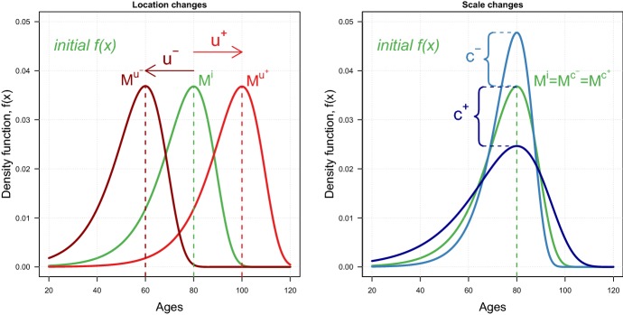
The role of the location and scale parameters can be easily understood with an illustration. Figure 1 shows the effects of changes in the two parameters on the density function of the LS family of mortality models.

Fig. 1.

Illustration of changes in the location u (left) and scale c (right) parameters on the density function f(x) of the location–scale family of mortality models. The density corresponds to the Gompertz model, and changes for u are from 80 to 60 ($u^{-}$) and 100 ($u^{+}$) and for c from 10 to 7.7 ($c^{-}$) and 15 ($c^{+}$). M denotes the old-age modal age at death.

Source: (Figs. 1 and 2) authors’ own elaborations

The location parameter u shifts the density function f(x) along the x-axis without altering its shape. In the left panel of Fig. 1, an increase (decrease) in u shifts the initial density to the right (left): this effect can be interpreted as a postponement (anticipation) of mortality. As such, changes in the parameter u correspond to a pure shifting effect that is a shift of the density to older (younger) ages, without any shape changes.

The scale parameter c affects the variability of the density function. In the right panel of Fig. 1, a decrease (increase) in c results in a compression (expansion) of the initial density around the old-age modal age at death M (the adult age at which most of the deaths occur). As such, changes in the parameter c correspond to a pure compression effect.

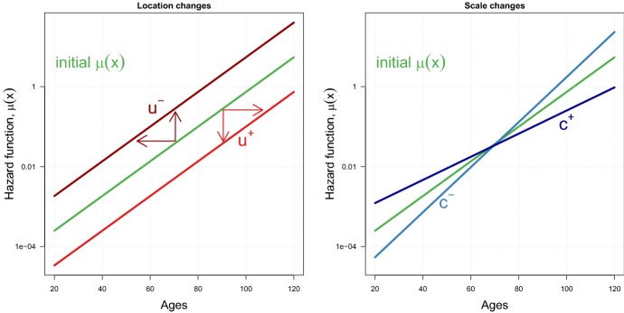
Figure 2 shows the corresponding effects of these changes on the force of mortality $\mu (x)$. In the left panel, location changes correspond to shifts of the mortality pattern (which are parallel for the Gompertz case shown in the figure); increases in u move $\mu (x)$ to the right (or down), while decreases in u result in left (or upwards) shifts. In the right panel, changes in the scale parameter modify the slope of the mortality pattern. This effect can be interpreted as a change in the “speed” of mortality: a decrease (increase) in c accelerates (slows down) the ageing process, so that mortality increases at a faster (lower) rate.

Fig. 2.

Illustration of changes in the location u (left panel) and scale c (right panel) parameters on the force of mortality $\mu (x)$ of the location–scale family of mortality models. The force of mortality corresponds to the Gompertz model, and changes for u and c are the same as shown in Fig. 1

The location and scale parameters thus capture and disentangle the shifting and compression dynamics of mortality. While we have shown the two effects in isolation for illustrative purposes, mortality changes typically occur simultaneously, and the two parameters can vary at the same time.

We can now proceed to show that several mortality models used in the demographic and actuarial literature belong to the LS family of mortality models. We first show this with a detailed derivation for the Gompertz model in the next section (and for the Weibull model in Appendix A). Then, we present a summary table of the mortality models that can be reconciled with the LS family in Sect. 2.4.

Gompertz and the Location–Scale Family

A model that is often used in demographic and actuarial analysis is the Gompertz model. This is one of the earliest attempts to find a “law of mortality”: at the beginning of the nineteenth century, Gompertz (1825) discovered that for a large part of the age range (though not including infancy and youth or very old ages) the force of mortality increases with age at a steady exponential rate. The Gompertz model is generally expressed in the form:

$$\begin{array}{c}\hfill \mu (x)=a{\text{e}}^{\mathit{bx}},x\ge 0,\end{array}$$ 5

where $a>0$ denotes the level of the force of mortality at the starting age of the analysis and b corresponds to the rate of ageing (Thatcher et al. 1998). From the life table functions introduced in Sect. 2.1, we can derive the density function f(x) of the Gompertz model:

$$\begin{array}{c}\hfill f(x)=\mu (x)l(x)=\mu (x){\text{e}}^{-{\int }_0^x\mu (a)da}=a\text{exp}\left[b,x,-,\frac{a}{b},({\text{e}}^{\mathit{bx}}-1)\right].\end{array}$$ 6

It is possible to show that the Gompertz model is closely related to the location–scale (LS) family of mortality models. In particular, the LS-like parameterization of the Gompertz model for the force of mortality is

$$\begin{array}{c}\hfill \mu (x)=\frac{1}{c}{\text{e}}^{\frac{x-u}{c}},x\ge 0,\end{array}$$ 7

where $u\in \mathbb{R}$ and $c>0$ are the location and scale parameters, respectively. The corresponding LS-like density function of the Gompertz model can be expressed as:

$$\begin{array}{c}\hfill f(x)=\frac{1}{c}\text{exp}\left[\frac{x-u}{c},-,\text{exp},\left(\frac{x-u}{c}\right),+,\text{exp},\left(-,\frac{u}{c}\right)\right].\end{array}$$ 8

Indeed, if we let the location and scale parameters be $u=\frac{1}{b}ln\left(\frac{b}{a}\right)$ and $c=\frac{1}{b}$, and we substitute them in Eqs. (7) and (8), we obtain the classic Gompertz formulas in Eqs. (5) and (6).

The Gompertz model does not strictly belong to the LS family of mortality models: its force of mortality is only defined for $x\ge 0$, while the location–scale $\mu (x)$ can vary on the entire set $\mathbb{R}$ (see Eq. (3)). The truncation of the x-axis can be also observed in the functional form of f(x) in Eq. (8), which depends on the parameters u and c via the $\text{exp}\left({\text{e}}^{-\frac{u}{c}}\right)$ term. Nevertheless, the Gompertz model is closely related to a location–scale distribution, the Gumbel (or type 1 extreme–value distribution, Johnson et al. 1995): “the Gompertz distribution is a special case of the Gumbel distribution for the minima, i.e. when$x:=-x$and truncated at$x=0$” (Lenart and Missov 2016, p. 2923). As such, the Gompertz model can be considered a truncated location–scale distribution.

The location and scale parameters of the Gompertz model are reported in Table 1 of the following section, together with the formulas of the classic and LS-like $\mu (x)$; the classic and LS-like functional forms of f(x) are reported in Table 3 of Appendix B.

Table 1.

Mortality models belonging to the location–scale (LS) and log–location–scale (LLS) families and models closely related to them, together with their parameterization in terms of the classic, LS and LLS force of mortality $\mu (x)$, ${\mu }_{\mathrm{LS}}(x)$, ${\mu }_{\mathrm{LLS}}(x)$, location u and scale c parameters

Models belonging to the LS family	$\mu (x)$	$\frac{1}{c}{\mu }_{\mathrm{LS}}\left(\frac{x-u}{c}\right)$	u	c
Logistic	$\frac{b\text{exp}(a+bx)}{1+\text{exp}(a+bx)}$	$\frac{1}{c}\frac{\text{exp}(\frac{x-u}{c})}{1+\text{exp}(\frac{x-u}{c})}$	$-\frac{a}{b}$	$\frac{1}{b}$
Normal	$\frac{1}{\sigma }\frac{\varphi \left(\frac{x-\lambda }{\sigma }\right)}{1-\mathrm{\Phi }\left(\frac{x-\lambda }{\sigma }\right)}$	$\frac{1}{c}\frac{\varphi \left(\frac{x-u}{c}\right)}{1-\mathrm{\Phi }\left(\frac{x-u}{c}\right)}$	$\lambda$	$\sigma$
Smallest Extreme–Value	$\frac{1}{\sigma }\text{exp}(\frac{x-\lambda }{\sigma })$	$\frac{1}{c}\text{exp}(\frac{x-u}{c})$	$\lambda$	$\sigma$
Largest Extreme–Value	$\frac{1}{\sigma }\frac{\text{exp}(-\frac{x-\lambda }{\sigma })}{\text{exp}\left[\text{exp},\left(-,\frac{x-\lambda }{\sigma }\right)\right]-1}$	$\frac{1}{c}\frac{\text{exp}(-\frac{x-u}{c})}{\text{exp}\left[\text{exp},\left(-,\frac{x-u}{c}\right)\right]-1}$	$\lambda$	$\sigma$

Models belonging to the LLS family	$\mu (x)$	$\frac{1}{cx}{\mu }_{\mathrm{LLS}}\left(\frac{ln(x)-u}{c}\right)$	u	c
Weibull	$ab{(ax)}^{b-1}$	$\frac{1}{cx}\text{exp}\left(\frac{ln(x)-u}{c}\right)$	$-ln(a)$	$\frac{1}{b}$
Log–Logistic	$\frac{b}{x}\frac{\text{exp}(a+bln(x))}{1+\text{exp}(a+bln(x))}$	$\frac{1}{cx}\frac{\text{exp}\left(\frac{ln(x)-u}{c}\right)}{1+\text{exp}\left(\frac{ln(x)-u}{c}\right)}$	$-\frac{a}{b}$	$\frac{1}{b}$
Log–Normal	$\frac{1}{\sigma x}\frac{\varphi \left(\frac{ln(x)-\lambda }{\sigma }\right)}{1-\mathrm{\Phi }\left(\frac{ln(x)-\lambda }{\sigma }\right)}$	$\frac{1}{cx}\frac{\varphi \left(\frac{ln(x)-u}{c}\right)}{1-\mathrm{\Phi }\left(\frac{ln(x)-u}{c}\right)}$	$\lambda$	$\sigma$

Models related to the LS family	$\mu (x)$	LS-like $\mu (x)$	u	c
Gompertz	$a\text{exp}(bx)$	$\frac{1}{c}\text{exp}\left(\frac{x-u}{c}\right)$	$\frac{1}{b}ln\left(\frac{b}{a}\right)$	$\frac{1}{b}$
Gamma–Gomp	$\frac{a\text{exp}(bx)}{1+\frac{a}{b}\gamma \left[\text{exp},(,b,x,),-,1\right]}$	$\frac{1}{c}\frac{\text{exp}\left(\frac{x-u}{c}\right)}{1+\gamma \left[\text{exp},\left(\frac{x-u}{c}\right),-,,\text{exp},\left(-,\frac{u}{c}\right)\right]}$	$\frac{1}{b}ln\left(\frac{b}{a}\right)$	$\frac{1}{b}$
Kannisto	$\frac{\text{exp}(a+bx)}{1+\text{exp}(a+bx)}$	$\frac{\text{exp}(\frac{x-u}{c})}{1+\text{exp}(\frac{x-u}{c})}$	$-\frac{a}{b}$	$\frac{1}{b}$
Minimal Generalized Extreme–Value	$\frac{1}{\sigma }{\left[1,+,\xi ,\left(-,\frac{x-\lambda }{\sigma }\right)\right]}^{-\frac{1}{\xi }-1}$	$\mu (x)$	$\lambda$	$\sigma$
Maximal Generalized Extreme–Value	$\frac{1}{\sigma }\frac{\text{exp}\left(-,s^{-\frac{1}{\xi }}\right)s^{-\frac{1}{\xi }-1}}{1-\text{exp}\left(-,s^{-\frac{1}{\xi }}\right)}$	$\mu (x)$	$\lambda$	$\sigma$
	where $s=1+\xi \left(\frac{x-\lambda }{\sigma }\right)$

$\varphi (z)=\frac{1}{\sqrt{2\pi }}\text{exp}\left(-,\frac{z^2}{2}\right)$ and $\mathrm{\Phi }(z)={\int }_{-\infty }^z\varphi (w)\mathrm{d}w$ denote the probability density function and the cumulative distribution function of the standardized normal distribution, respectively

Table 3.

Mortality models belonging to the location–scale (LS) and log–location–scale (LLS) families and models closely related to them, together with their parameterization in terms of the classic, LS and LLS functional forms f(x), $f_{\mathrm{LS}}(x)$ and $f_{\mathrm{LLS}}(x)$

Models belonging to the LS family	f(x)	$\frac{1}{c}{f}_{\mathrm{LS}}\left(\frac{x-u}{c}\right)$
Logistic	$\frac{b\text{exp}(a+bx)}{{\left[1,+,\text{exp},(,a,+,b,x,)\right]}^2}$	$\frac{1}{c}\frac{\text{exp}(\frac{x-u}{c})}{{\left[1,+,\text{exp},(,\frac{x-u}{c},)\right]}^2}$
Normal	$\frac{1}{\sigma }\varphi (\frac{x-\lambda }{\sigma })$	$\frac{1}{c}\varphi (\frac{x-u}{c})$
Smallest Extreme–Value	$\frac{1}{\sigma }\text{exp}\left[\frac{x-\lambda }{\sigma },-,\text{exp},\left(\frac{x-\lambda }{\sigma }\right)\right]$	$\frac{1}{c}\text{exp}\left[\frac{x-u}{c},-,\text{exp},\left(\frac{x-u}{c}\right)\right]$
Largest Extreme–Value	$\frac{1}{\sigma }\text{exp}\left[-,\frac{x-\lambda }{\sigma },-,\text{exp},\left(-,\frac{x-\lambda }{\sigma }\right)\right]$	$\frac{1}{c}\text{exp}\left[-,\frac{x-u}{c},-,\text{exp},\left(-,\frac{x-u}{c}\right)\right]$

Models belonging to the LLS family	f(x)	$\frac{1}{cx}{f}_{\mathrm{LLS}}\left(\frac{ln(x)-u}{c}\right)$
Weibull	$ab{(ax)}^{b-1}\text{exp}\left[-,{(ax)}^b\right]$	$\frac{1}{cx}\text{exp}\left[\frac{ln(x)-u}{c},-,\text{exp},\left(\frac{ln(x)-u}{c}\right)\right]$
Log–Logistic	$\frac{b}{x}\frac{\text{exp}(a+bln(x))}{{\left[1,+,\text{exp},(,a,+,b,ln,(,x,),)\right]}^2}$	$\frac{1}{cx}\frac{\text{exp}(\frac{ln(x)-u}{c})}{{\left[1,+,\text{exp},(,\frac{ln(x)-u}{c},)\right]}^2}$
Log–Normal	$\frac{1}{\sigma x}\varphi (\frac{ln(x)-\lambda }{\sigma })$	$\frac{1}{cx}\varphi (\frac{ln(x)-u}{c})$

Models related to the LS family	f(x)	LS-like f(x)
Gompertz	$a\text{exp}\left[b,x,-,\frac{a}{b},({\text{e}}^{\mathit{bx}}-1)\right]$	$\frac{1}{c}\text{exp}\left[\frac{x-u}{c},-,\text{exp},\left(\frac{x-u}{c}\right),+,\text{exp},\left(-,\frac{u}{c}\right)\right]$
Gamma–Gomp	$\frac{a\text{exp}(bx)}{{\left\{1,+,\frac{a}{b},\gamma ,\left[\text{exp},(,b,x,),-,1\right]\right\}}^{\frac{1}{\gamma }+1}}$	$\frac{1}{c}\frac{\text{exp}\left(\frac{x-u}{c}\right)}{{\left\{1,+,\gamma ,\left[\text{exp},\left(\frac{x-u}{c}\right),-,\text{exp},\left(-,\frac{u}{c}\right)\right]\right\}}^{\frac{1}{\gamma }+1}}$
Kannisto	$\frac{\text{exp}(a+bx)}{{\left[1,+,\text{exp},(,a,+,b,x,)\right]}^{\frac{1}{b}+1}}$	$\frac{\text{exp}(\frac{x-u}{c})}{{\left[1,+,\text{exp},(,\frac{x-u}{c},)\right]}^{1+c}}$
Minimal Generalized Extreme–Value	$\frac{1}{\sigma }\frac{\text{exp}\left\{-,{\left[1,+,\xi ,\left(-,\frac{x-\lambda }{\sigma }\right)\right]}^{-\frac{1}{\xi }}\right\}}{{\left[1,+,\xi ,\left(-,\frac{x-\lambda }{\sigma }\right)\right]}^{\frac{1}{\xi }+1}}$	$\frac{1}{c}\frac{\text{exp}\left\{-,{\left[1,+,\xi ,\left(-,\frac{x-u}{c}\right)\right]}^{-\frac{1}{\xi }}\right\}}{{\left[1,+,\xi ,\left(-,\frac{x-u}{c}\right)\right]}^{\frac{1}{\xi }+1}}$
Maximal Generalized Extreme–Value	$\frac{1}{\sigma }\frac{\text{exp}\left\{-,{\left[1,+,\xi ,\left(\frac{x-\lambda }{\sigma }\right)\right]}^{-\frac{1}{\xi }}\right\}}{{\left[1,+,\xi ,\left(\frac{x-\lambda }{\sigma }\right)\right]}^{\frac{1}{\xi }+1}}$	$\frac{1}{c}\frac{\text{exp}\left\{-,{\left[1,+,\xi ,\left(\frac{x-u}{c}\right)\right]}^{-\frac{1}{\xi }}\right\}}{{\left[1,+,\xi ,\left(\frac{x-u}{c}\right)\right]}^{\frac{1}{\xi }+1}}$

$\varphi (z)=\frac{1}{\sqrt{2\pi }}\text{exp}\left(-,\frac{z^2}{2}\right)$ denotes the probability density function of the standardized normal distribution

Finally, it is interesting to observe that, if we let the location parameter be equal to the old-age modal age at death M, that is $u=M$, and we keep $c=\frac{1}{b}$, then Eq. (7) becomes:

$$\begin{array}{c}\hfill \mu (x)=b{\text{e}}^{b(x-M)},\end{array}$$ 9

which is the parameterization of the Gompertz model in terms of the modal age at death (Horiuchi et al. 2013; Missov et al. 2015).

Other Parametric Mortality Models

Several models have been proposed to describe the age pattern of the force of mortality during the last two centuries (for a comprehensive review, see Tabeau 2001), and many of them can be unified under the overarching family of location–scale models. Table 1 presents twelve well-known models of mortality that either belong to the location–scale (LS) and log–location–scale (LLS) families or that are closely related to them. The table reports each model’s parameterization in terms of the classic and LS force of mortality $\mu (x)$, ${\mu }_{\mathrm{LS}}(x)$ or ${\mu }_{\mathrm{LLS}}(x)$, location u and scale c parameters. The classic and LS functional form f(x) $f_{\mathrm{LS}}(x)$ or $f_{\mathrm{LLS}}(x)$ is reported in Table 3 in Appendix B.

A first interesting observation is that the Smallest Extreme–Value (Gumbel distribution for the minima) and the Gompertz model are characterized by the same hazard function. However, as already discussed in the previous section, only the former strictly belongs to the LS family due to the truncation of the x-axis in the latter.

The Kannisto, Gamma–Gompertz, Minimal and Maximal Generalized Extreme–Value models do not strictly belong, but are closely related to the LS family. First, the Kannisto model is specified by an unscaled logistic hazard function (which is equal to the Logistic model except for the $\frac{1}{c}$ term, see Table 1), and it has been extensively employed to smooth mortality at older ages (for example, Wilmoth et al. 2007; Ševčíková et al. 2016). Second, the Gamma–Gompertz is a three-parameter model that includes the Kannisto as a special case: its hazard function has a logistic shape whose asymptote can be different than one. Also this model has gained relevant prominence during the last decades (Vaupel et al. 1979; Missov and Lenart 2013; Colchero et al. 2016). Finally, the Minimal and Maximal Generalized Extreme–Value models are characterized by three parameters, and for a fixed value of the third parameter (i.e. $\xi$), their force of mortality satisfies Eq. (3).

The three models belonging to the LLS family (Weibull, Log–Logistic and Log–Normal) are generally used in the analysis of survival data rather than portraying the human mortality pattern. Nevertheless, they are characterized by two important demographic properties related to the longevity and lifespan inequality of the population under their mortality pattern assumption (for additional details, see Gigliarano et al. 2017).

Finally, it is interesting to note that the three models of the LLS family have the property that the transformation $Y=\text{log}(X)$ belongs to the location–scale class. Indeed, the Weibull, Log–Logistic and Log–Normal models for X correspond to the Smallest Extreme–Value, Logistic and Normal models for Y (Lawless 2011).

Data and Estimation Procedure

For the illustrations shown in this article, we use available data from the Human Mortality Database (HMD 2018). In particular, we employ death counts $D_x$ and exposure to risk $E_x$ in single years of age x for all the HMD countries that have available data starting from the year 1960 to keep the time range of the analysis sufficiently long.

This results in a subset of 33 countries (and 39 populations): Australia, Austria, Belarus, Belgium, Bulgaria, Canada, Czech Republic, Denmark, Estonia, Finland, France, East and West Germany, Hungary, Iceland, Ireland, Italy, Japan, Latvia, Lithuania, Luxembourg, Netherlands, New Zealand (total, Maori and non-Maori population), Norway, Poland, Portugal, Russia, Slovakia, Spain, Sweden, Switzerland, UK (total population, England and Wales, Scotland and Northern Ireland), Ukraine and the USA. The remaining countries of the HMD (Chile, Germany total population, Greece, Israel, Slovenia and Taiwan) are not considered due to shorter mortality series. In the illustration in Sect. 3.1, we focus only on a subset of four high-longevity countries, namely Denmark, Japan, Sweden and the USA.

It should be further noted that the data employed here are the unsmoothed deaths and person-years from the HMD. As such, model fitting occurs on actual rather than adjusted data, and goodness of fit depends uniquely on the ability of the model to capture observed unadjusted mortality trends.

To estimate the parameters of a model, be it expressed in the classic or in the location–scale (LS) parameterization, we assume that death counts $D_x$ at a given age x follow a Poisson distribution (Brillinger 1986):

$$\begin{array}{c}\hfill D_x\sim \mathcal{P}(E_x{\mu }_x(\mathit{\theta })),\end{array}$$ 10

where ${\mu }_x(\mathit{\theta })$ is the parametric hazard function of interest, $\mathit{\theta }$ is the vector of the model’s parameters (classic or LS) and $E_x$ is the exposure to risk. Under this assumption, the parameters can be estimated by maximizing the following log-likelihood function:

$$\begin{array}{c}\hfill ln\mathcal{L}\left(\mathit{\theta }|,D_x,,,E_x\right)\propto \sum _{x=\alpha }^{\beta }\left\{D_x,,ln,\left({\mu }_x,(\mathit{\theta })\right),-,E_x,,{\mu }_x,(\mathit{\theta })\right\},\end{array}$$ 11

where $\alpha$ and $\beta$ denote the lowest and highest age groups in the analysis, respectively. The estimation of the model’s parameters is carried out by maximizing Eq. (11) in R (R Development Core Team 2017) either with the standard general-purpose numerical optimizer optim or with the package DEoptim (Mullen et al. 2011). Routines for fitting the models of the LS family are available in the Supplementary material.

Illustrations

Parameter Interpretation: Shifting and Compression

An important demographic question that can be directly studied with the location–scale (LS) family is the assessment of the shifting and compression dynamics of mortality changes. The estimation of the LS parameters over a specified time interval indeed allows to visually inspect the level and trend of each dynamic within the overall mortality development.

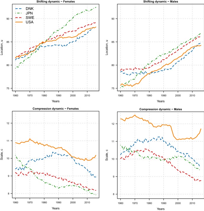
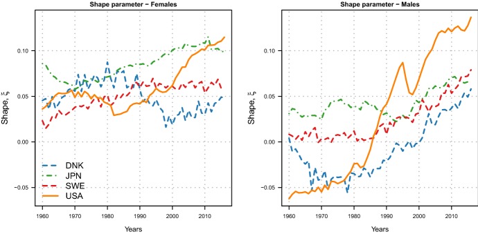
Here, we illustrate this property of the LS family by assessing the evolution of the two dynamics in four high-longevity countries, namely Denmark, Japan, Sweden and the USA. For each country, we fitted all the models of the LS family for adult females and males aged 30–110+ during 1960–2016, and we selected the best fitting model using the Bayesian Information Criterion (BIC, Schwarz 1978, see Appendix C for additional details and computational procedure). The Minimal Generalized Extreme–Value (MinGEV) model is the best specification for both genders in the four countries (see Table 4 in Appendix D for the BIC and rankings of the different models). Figure 3 shows the estimated location u and scale c parameters, while the shape estimates are reported in Fig. 9 in Appendix D.

Table 4.

BIC values (divided by 100) of nine LS models for adult females and males in Denmark, Japan, Sweden and the USA, 1960–2016

Model	DNK		JPN		SWE		USA
	F	M	F	M	F	M	F	M
MinGEV	106	81	2172	799	203	105	1738	1331
Ga–Go	128	84	4607	1237	295	130	3693	2318
Gomp	142	92	5240	1433	309	137	4937	3989
Kann	236	111	7182	2529	476	232	8774	5829
Weib	775	479	22,265	13,026	1533	1110	36,699	32,631
MaxGEV	1457	872	43,370	23,773	3373	2234	61,906	37,915
Logis	1951	1507	32,937	25,744	3457	2934	76,047	60,910
Norm	2546	1824	57,583	37,984	5268	4027	102,331	71,574
LargEV	8116	6986	149,526	118,413	16,008	13,829	307,781	243,955

The models are listed by ascending order of BIC for Danish females

Fig. 3.

Estimated location u and scale c parameters of the Minimal Generalized Extreme–Value model for female (left) and male (right) adults aged 30–110+ in four high-longevity countries during 1960–2016.

Source (Figs. 3–11): authors’ calculations based on data from the Human Mortality Database (2018). (Color figure online)

Fig. 9.

Estimated shape $\xi$ parameters of the Minimal Generalized Extreme–Value model for female (left) and male (right) adults aged 30–110+ in four high-longevity countries during 1960–2016. (Color figure online)

From the top panels of Fig. 3, it is possible to determine the beginning of the shifting dynamic in the different countries by gender. For females, mortality started to shift before the 1960: indeed, the location parameter has been linearly increasing during all years in each country, albeit at different rates. Japanese females experienced the fastest rate of mortality postponement, which shows some signs of deceleration in most recent years; in addition, a lack of shifting mortality for Danish females clearly emerges during 1980–1995, a period coinciding with their stagnation of life expectancy (Christensen et al. 2010; Lindahl-Jacobsen et al. 2016a, b). For males, the postponement of mortality started at different points in time in the four countries: while Japan was already experiencing this dynamic during the 1960s, the postponement started in the early 1970s in the USA, in the early 1980s in Sweden and in the early 1990s in Denmark.

From the bottom panels of Fig. 3, the compression dynamic of mortality can be assessed (decreasing values of c correspond to compression). For females, a linear decreasing trend can be observed in Sweden and the USA, starting around the 1970s; in Japan, the decrease is very rapid until the 1990s, after which a period of stagnation occurred; and in Denmark, mortality first expanded for about 20 years at the beginning of the period (1965–1985), and then, it started to compress again. For males, very different trends of compression, stagnation and expansion can be observed at different points in time.

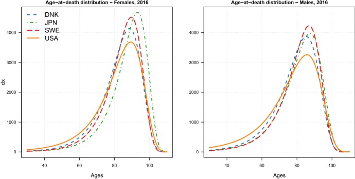
On top of assessing changes in the two dynamics, the LS parameters readily allow a cross-country comparison on the level of the two dynamics. A first interesting observation is that both females and males in the USA are lagging behind other countries in terms of both dynamics. The higher scale parameters in the USA correspond to a greater variability of the age-at-death distribution, which translates into a higher number of “premature” deaths (i.e. deaths occurring at young adult ages). Figure 10 in Appendix D reports the estimated MinGEV age-at-death distributions in 2016 for the four countries: the share of premature deaths for the USA females and males is indeed higher than for the other three countries.

Fig. 10.

Age-at-death distributions in 2016 for female (left) and male (right) adults aged 30–110+ in four high-longevity countries corresponding to the Minimal Generalized Extreme–Value model estimates

Another interesting observation is that location parameters for Denmark are below those for Sweden, while the scale parameters are higher. A possible interpretation is that the different smoking behaviour of Danish and Swedish has been a major reason for this difference. Denmark is one of the few high-income countries that experienced stagnation in life expectancy in recent decades (Lindahl-Jacobsen et al. 2016b), which was paralleled by stagnation in lifespan inequality. Smoking has been indicated as the single most important factor in explaining the lower life expectancy (Sundhedsministeriet 1994; Jacobsen et al. 2004, 2006; Lindahl-Jacobsen et al. 2016a) and the higher lifespan disparity in Denmark compared to Sweden (Aburto et al. 2018).

Furthermore, Japanese women experienced the greatest shift of mortality as well as more compression compared to the other countries. The very fast improvements in mortality since the end of the Second World War have brought them to be the “best practice” or most longevous population worldwide since the 1980s (see Oeppen and Vaupel 2002, Fig. 2). The Japanese age profile of mortality has been shaped from over 35 years of best practice population and is unique even among the closely competing countries such as South Korea and Hong Kong (Vallin and Meslé 2016; Kontis et al. 2017).

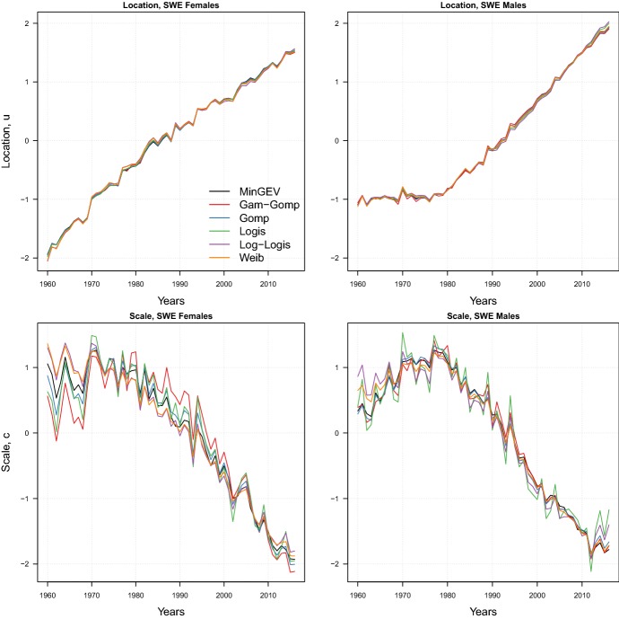
Two important points are worth being mentioned here. First, the assessment of the shifting and compression dynamics would be the same if we had employed a different model of the LS family. Figure 11 in Appendix D shows the location u and scale c rescaled estimates for six models of the LS family fitted on Swedish adult females and males. The figure shows that the location and scale estimates are very consistent across models: the same patterns of shifting and compression dynamics emerge from the different LS models. Second, time trends of the location and scale parameters for the USA and Japan are in line with the empirical findings of shift and compression illustrated by Canudas-Romo (2008) and Ouellette and Bourbeau (2011): trends of the modal age at death and of the variability around (in the former) and above (in the latter) the mode closely resemble our results. Moreover, the trends of u for Swedish and Danish females are remarkably similar to the trends of their temporary life expectancy between ages 50 and 85 (see Lindahl-Jacobsen et al. 2016a, Fig. 1a).

Fig. 11.

Location u and scale c rescaled estimates of six LS models for female and male adults aged 30–110+ in Sweden during 1960–2016

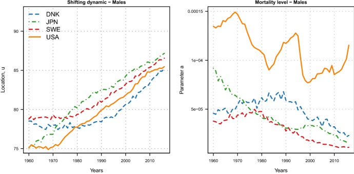
The analyses above, and in particular the assessment of the shifting dynamic, could not be performed based on the classic formulation of parametric models shown in the first column of Table 1. Figure 4 shows the Gamma–Gompertz (GG) estimates of the parameters u (for the GG LS model) and a (for the classic GG model) for males in the same four countries during 1960–2016. The estimates of u for the GG LS model are very close to those of the MinGEV model shown in Fig. 3 (mean absolute percentage difference of 0.3%). In the right panel of Fig. 4, the time trend of the parameter a reflects changes in the level of the force of mortality at the starting age of the analysis. As such, it does not allow to disentangle mortality changes due to the shifting dynamic as captured by the u parameter in the left panel. The trends of the two parameters (after reverting u or a) are indeed not comparable: in the USA, for example, the trend of a is quite erratic, while the parameter u shows an unequivocal beginning of the shifting dynamic from the 1970s.

Fig. 4.

Estimated Gamma–Gompertz parameters u (LS model, left) and a (classic model, right) for male adults aged 30–110+ in four high-longevity countries during 1960–2016. Note: The y-axis of the left panel is identical to the one in the upper right panel of Fig. 3 for comparison purposes. (Color figure online)

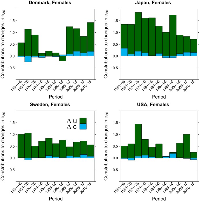
Finally, we present a decomposition of mortality changes into shift and compression effects for the four countries. Our methodology is based and extends the decomposition method introduced by Bergeron-Boucher et al. (2015) to the LS-like parameterization of the Gompertz model. Appendix E reports the formulas and computational procedures that we have used for this analysis. Figure 5 shows the decomposition of changes in life expectancy at age 30 by location (shifting) and scale (compression) contributions in the Gompertz model for females in the four countries from 1960 until 2015 in 5-year intervals.

Fig. 5.

Trends over time of the contributions of the location u (green) and scale c (light blue) Gompertz parameters to changes in female life expectancy at age 30 for females in Denmark, Japan, Sweden and the USA, 1960–2015. (Color figure online)

The figure shows that changes in the location parameter, hence shifting mortality, are the main components driving changes in life expectancy during the period 1960–2015. Conversely, the contributions of changes in the scale parameter are limited and even negatives in some periods. With respect to our previous discussions, the stagnation of the location parameter for Danish females between 1977 and 1995 is reflected in the small changes in life expectancy during this period. Moreover, the fast increase in the location parameter experienced by Japanese females has been the main contributor to the remarkable gains in life expectancy. These results are in line with those reported by Bergeron-Boucher et al. (2015, Fig. 7, Appendix C).

Correlation and Bias of Parameter Estimates

It is well known that a high correlation between the estimators of model parameters is an undesirable property, as “it shows a kind of inaccuracy of the estimators” (Gupta and Székely 1994, p. 588). Reducing the correlation of the maximum likelihood estimators (MLE) of parametric models is therefore a beneficial task, as it improves parameter interpretability and reduces estimation bias. In particular, Gupta and Székely (1994) have shown that location–scale distributions can generally be re-parameterized so that the maximum likelihood estimators are asymptotically independent.

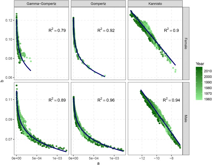
Missov et al. (2015) have shown that the MLE of the parameters a and b of the classic Gompertz model in Eq. (5) are highly (negatively) correlated. This is in general true for the parametric models in Table 1 that are expressed in their classic notation $\mu (x)$. Figure 6 shows the MLE of the typical a and b parameters of the Gamma–Gompertz, Gompertz and Kannisto mortality models for the thirty-three Human Mortality Database (HMD) countries listed above from 1960 until the most recent year by gender. Each point on the graph corresponds to a set of estimated parameters for a single country in a given year.

Fig. 6.

Maximum likelihood estimates and $R^2$ of a linear model for the classic parameters a and b for the Gamma–Gompertz, Gompertz and Kannisto model for thirty-three HMD countries from 1960 until the most recent year by gender. The a parameter was transformed in $a^{0.1}$ to linearize the relationship for the two Gompertz cases

The estimated parameter b tends to decrease as a increases for all models, following a power function for the two Gompertz’s specifications and a linear function for the Kannisto model. The variability around the two estimated parameters is very small: indeed, the $R^2$ of a linear model between a and b (after a suitable power transformation of the parameter a for the two Gompertz cases) is always very high (average $R^2$ of 0.90).

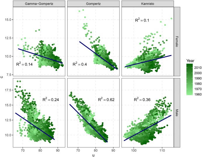
This rather high correlation between the estimators of classic parametric models can be reduced by re-parameterizing them in terms of the LS family. Figure 7 shows the MLE of the LS parameters u and c for the same models, countries and years by gender. From the graphs, it is clear that the relationship between the LS estimates is much weaker than for the classic ones. The variability around the LS parameters is higher, and the $R^2$ of the linear regression between u and c is significantly reduced (average $R^2$ of 0.31). Furthermore, the relationship is not always negative as in the previous case: for the Kannisto model, increases in u tend to correspond to increases in c.

Fig. 7.

Maximum likelihood estimates and $R^2$ of a linear model for the LS parameters u and c for the Gamma–Gompertz, Gompertz and Kannisto model for thirty-three HMD countries from 1960 until the most recent year by gender

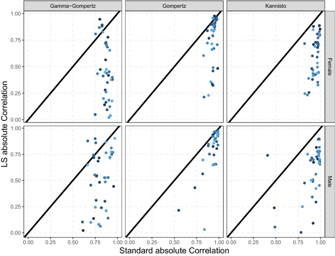
The weaker relationship of the LS estimates between countries is generated by a lower correlation of u and c with respect to a and bwithin countries. Figure 8 shows the within-country absolute correlation of the two set of estimated parameters for the three models: each point on the graph corresponds to the absolute correlation of the classic and LS parameters within one country during all the years considered in the analysis (1960 until the most recent available year) by gender. The great majority of points in Fig. 8 fall below the diagonal, confirming that the absolute correlation between estimators of classic models’ parameter can be significantly reduced by using the LS family.

Fig. 8.

Within-country absolute correlation of the classic and LS parameterization of the Gamma–Gompertz, Gompertz and Kannisto model for thirty-three HMD countries from 1960 until the most recent year by gender

Finally, we perform an experiment that demonstrates the reduction in estimation bias when using the LS family versus the classic models’ parameterization. Specifically, we consider Swedish adult female mortality in 2000, and we estimate the Weibull, Logistic and Gompertz LS parameters u and c. We consider these estimates to be the “true” model parameters, and we derive the corresponding true a and b of the classic models via the formulas in Table 1. Then, we produce 100 simulations of age-specific Poisson death counts using the true hazard and the observed exposure times. For each simulation, we estimate the LS and classic model’s parameters, and we compute the relative absolute bias (AB) for each parameter $\theta$ using the formula:

$$\begin{array}{c}\hfill \text{AB}=\frac{|\widehat{\theta }-\theta |}{\theta },\end{array}$$ 12

where $\widehat{\theta }$ is the estimated value of the true parameter $\theta$ (Pletcher 1999). Table 2 reports the AB averaged over 100 simulations for the classic and LS parameters’ estimates of the Weibull, Logistic and Gompertz models.

Table 2.

Relative absolute bias (AB, in percentage terms) averaged over 100 simulations for the Weibull, Logistic and Gompertz classic parameters a and b, and the LS parameters u and c estimated on simulated Swedish adult female deaths in 2000

Model	AB
	a	b	u	c
Weibull	0.043	0.294	0.001	0.005
Logistic	0.344	0.352	0.044	0.351
Gompertz	3.048	0.327	0.037	0.326

The table shows that the AB for the LS estimates is always lower than for the classic model parameterization: employing the LS formulas improves the precision of parameters’ estimates. These results are in line with those of Missov et al., who performed a somewhat similar simulation experiment for the Gompertz model and showed that “a model misspecification leads to a relatively small bias in estimatedM [i.e. u in the LS framework] in comparison to the bias in the estimateda” (Missov et al. 2015, p. 1039).

Discussion and Conclusion

In this article, we have shown that many mortality models used in the demographic and actuarial literature can be re-parameterized in terms of a general and flexible family of models, the family of location–scale (LS) models. The models belonging to this family are characterized by two parameters that have a direct demographic interpretation: the location and scale parameters capture the shifting and compression dynamics of mortality changes.

The study of compression and shifting mortality is an important issue in demographic research, as both dynamics translate differently into survival function, mortality density and hazard distributions (Bergeron-Boucher et al. 2015). Mortality compression is associated with a rectangularization of the survival curve and with decreasing variability in the distribution of ages at death (Wilmoth and Horiuchi 1999; Cheung et al. 2005). Mortality shifting is associated with a parallel shift of the force of mortality to lower ages (Bongaarts 2005) and of the death distribution to higher ages (Canudas-Romo 2008), while retaining their original shape. As we have shown in Sect. 3.1, the estimation of the parameters of the LS family allows an assessment of the level and trend of these two mortality dynamics.

As such, re-parameterizing classic models in their LS formulation is very useful in aiding parameter interpretability and comparability across different populations. We have shown as illustration in Sect. 3.1 the analysis of the shifting and compression dynamics of mortality changes in four high-longevity countries by gender during 1960–2016: the LS estimated parameters readily allow to examine and compare the two dynamics within and between countries.

In addition, the LS parameterization has an important statistical advantage over classic models: the rather high correlation between estimators of classic models’ parameterization is significantly reduced within the LS framework, and thus, statistical estimation is facilitated. The lower correlation, in turn, further improves parameter interpretability and reduces estimation bias. As an illustration, we have shown in Sect. 3.2 that the correlation of the classic Gamma–Gompertz, Gompertz and Kannisto parameters for females and males aged 30–110+ in thirty-three Human Mortality Database countries is significantly higher than the LS parameterization, both within and between countries. Moreover, we performed simulation experiments to demonstrate the reduction in estimation bias for the Weibull, Logistic and Gompertz models when using the LS framework instead of the classic models’ formulas.

Another potentially important advantage deriving from the lower correlation is that the LS parameters could be forecasted more appropriately. The main advantages of using parameterization functions for forecasting mortality are the smoothness of forecast rates across age and the interpretability of the model’s parameters (Bell 1997; Booth and Tickle 2008). Nevertheless, forecasting via well-known laws of mortality has been very limited due to the very high correlation between parameter’s estimators (Booth and Tickle 2008). The lower correlation of the LS estimators could thus overcome this relevant issue. Parametric forecasts of mortality obtained with classic and the LS models are beyond the scope of the current paper and will be explored and compared in future work.

Although we have shown that several mortality models belong to the LS family, it should be noted that the family does not embrace the full spectrum of parametric models. Additive hazard models developed for adult mortality (e.g. the Makeham and the Gamma–Gompertz–Makeham models) as well as for the entire age range, such as the Siler (1979), the Heligman and Pollard (1980) and the CoDe (de Beer and Janssen 2016) models, do not belong to the LS family.

Nevertheless, the LS family reconciles several parametric mortality models under a unique framework, it readily allows the assessment of the shifting and compression dynamics of mortality changes, and it aids statistical estimation due to lower correlation between estimates of the model parameters. In turn, the latter could be further exploited for forecasting purposes. Re-parameterizing classic demographic models in terms of the LS family therefore offers great advantages, and the family should be considered for parametric mortality analysis.

Electronic supplementary material

Below is the link to the electronic supplementary material.

Appendix A: Weibull and the Log–Location–Scale Family

Here, we provide a similar derivation of Sect. 2.3 to show that the Weibull model belongs to the log–location–scale (LLS) family of mortality models.

Among its various parameterizations, the Weibull model can be expressed in the form:

$$\begin{array}{c}\hfill \mu (x)=ab{(ax)}^{b-1},x>0,\end{array}$$ A.1

where $a>0$ and $b>0$ are parameters (Lawless 2011). From the life table functions introduced in Sect. 2.1, we can then derive the density function f(x) of the Weibull model:

$$\begin{array}{c}\hfill f(x)=\mu (x)l(x)=\frac{b}{x}{(ax)}^b\text{exp}\left[-,{(ax)}^b\right].\end{array}$$ A.2

The Weibull model can be re-parameterized in terms of the LLS family. In particular, the LLS Weibull model for the force of mortality is

$$\begin{array}{c}\hfill \mu (x)=\frac{1}{cx}{\mu }_{\mathrm{LLS}}\left(\frac{ln(x)-u}{c}\right)=\frac{1}{cx}\text{exp}\left(\frac{ln(x)-u}{c}\right),\end{array}$$ A.3

where $u\in \mathbb{R}$ and $c>0$ are the location and scale parameters, respectively. The corresponding LLS density function of the Weibull model can be expressed as:

$$\begin{array}{cc}\hfill f(x)& =\frac{1}{cx}{f}_{\mathrm{LLS}}\left(\frac{ln(x)-u}{c}\right)\hfill \\ \hfill & =\frac{1}{cx}\text{exp}\left[\frac{ln(x)-u}{c},-,\text{exp},\left(\frac{ln(x)-u}{c}\right)\right].\hfill \end{array}$$ A.4

Indeed, if we let the location and scale parameters be $u=-ln(a)$ and $c=\frac{1}{b}$, and we substitute them in Eqs. (A.3) and (A.4), we obtain the classic Weibull formulas in Eqs. (A.1) and (A.2). As such, the Weibull model belongs to the LLS family of mortality models defined in Eqs. (2) and (4).

Appendix B: Location–Scale Functional form of Twelve Parametric Models of Mortality

Table 3 presents the classic, location–scale (LS) and log–location–scale (LLS) functional forms f(x), $f_{\mathrm{LS}}(·)$ and $f_{\mathrm{LLS}}(·)$ of the mortality models presented in Sect. 2.4.

Appendix C: Derivation of the Best Fitting Parametric Model

The selection of the best fitting parametric model can generally be made along different metrics and criterion. In this article, the estimation of a model’s parameter is achieved by maximum likelihood (Sect. 2.5); within a Poisson framework, the Bayesian Information Criterion (BIC, Schwarz 1978) is therefore a natural metric to compare different models, as it provides a good trade-off between model parsimony and accuracy.

Specifically, within a Poisson framework, the deviance is often used as a measure of discrepancy between observed and fitted data, and it is defined as:

$$\begin{array}{c}\hfill \text{Dev}=2\sum _y\sum _x\left[D_{x,y},,ln,\left(\frac{D_{x,y}}{{\widehat{D}}_{x,y}}\right),-,(D_{x,y}-{\widehat{D}}_{x,y})\right],\end{array}$$ C.1

where $D_{x,y}$ and ${\widehat{D}}_{x,y}$ denote the observed and fitted number of deaths at age x and year y, respectively. This is a “badness of fit” measure, as higher values correspond to worse models in terms of goodness of fit.

In the two-dimensional age and time setting, the BIC can then be computed as:

$$\begin{array}{c}\hfill \text{BIC}=\text{Dev}+ln(mn)\text{ED}\end{array}$$ C.2

where m and n are the dimensions (length) of age and time, respectively. ED denotes the effective dimension, or total number of parameters, of a model. Lower BIC values are associated with better models, and the trade-off between accuracy and parsimony is accounted for by the two components of the BIC.

Appendix D: Section 3.1: Additional Results

Here, we present some additional results corresponding to the analyses of Sect. 3.1.

Table 4 shows the BIC and rankings of the different LS models. From the table, it emerges that the Minimal Generalized Extreme–Value (MinGEV) model is the best specification for both genders in the four countries.

Figure 9 shows the estimated shape $\xi$ parameters of the MinGEV model for the four countries by sex during 1960–2016.

Figure 10 shows the estimated MinGEV age-at-death distributions for the four countries by sex in 2016. From the figure, it is possible to observe that the share of premature deaths for the USA females and males is higher than for the other three countries. In addition, the smaller compression of the USA distribution of deaths compared to the other countries clearly emerges from the two graphs.

Figure 11 shows the location u and scale c estimates for six models of the LS family fitted to Swedish adult female and male mortality during 1960–2016. The parameters have been rescaled for comparability, and while here we focus on Sweden, the results are the same for the other countries.

The figure shows that the location and scale estimates are very consistent across models: the former are always extremely close to each other, as well as the latter which are characterized by a slightly higher volatility. As such, the very same patterns of shifting and compression dynamics emerge from employing different LS models due to the similarity of the models’ estimates.

Appendix E: Decomposition of Mortality Changes into Location and Scale Effects

Here, we decompose changes in life expectancy at age 30 (${\dot{e}}_{30,t}$) into two components:

$$\begin{array}{c}\hfill {\dot{e}}_{30,t}=\mathrm{\Delta }u+\mathrm{\Delta }c,\end{array}$$ E.1

where $\mathrm{\Delta }u$ and $\mathrm{\Delta }c$ are the gains in life expectancy resulting from the changes in the location (shift) and scale (compression) parameters, respectively.

Taking advantage of the findings reported in Fig. 11, namely the consistency and comparability of the location–scale parameters across different specification of the LS family, we focus on the decomposition of the Gompertz model. Specifically, we extend the methodology presented by Bergeron-Boucher et al. (2015) to the LS-like parameterization of the Gompertz model.

Equation (7) introduced the LS-like parameterization of the Gompertz model. Here, we make explicit the time dependency of the model by letting the location and scale parameters be a function of time t:

$$\begin{array}{c}\hfill {\mu }_{x,t}=\frac{1}{c_t}{\text{e}}^{\frac{x-u_t}{c_t}}.\end{array}$$ E.2

Let a dot on top of a variable denote its derivative with respect to time (Vaupel and Canudas-Romo 2003). The change over time in the force of mortality (${\dot{\mu }}_{x,t}$) can be decomposed into respective components of change for the location (${\dot{u}}_t$) and scale (${\dot{c}}_t$) parameters:

$$\begin{array}{cc}\hfill {\dot{\mu }}_{x,t}& ={\dot{u}}_t\left[-,\frac{{\mu }_{x,t}}{c_t}\right]+{\dot{c}}_t\left[-,\frac{{\mu }_{x,t}}{c_t},\left(1,+,\frac{x-u_t}{c_t}\right)\right]\hfill \\ \hfill & ={\dot{u}}_t{f}_u({\mu }_{x,t})+{\dot{c}}_t{f}_c({\mu }_{x,t}),\hfill \end{array}$$ E.3

where $f_u({\mu }_{x,t})$ and $f_c({\mu }_{x,t})$ are weighting function of the hazard rate for the location and scale parameters, respectively.

Similarly to the force of mortality, we can derive the time change of life expectancy. Specifically, life expectancy at age 30 can be expressed as:

$$\begin{array}{c}\hfill e_{30,t}={\int }_{30}^{\omega }{l}_{a,t}{d}_a,\end{array}$$ E.4

where $l_{a,t}$ is the survival function at age a and time t. Changes in life expectancy at age 30 (${\dot{e}}_{30,t}$) can thus be written as:

$$\begin{array}{c}\hfill {\dot{e}}_{30,t}={\int }_{30}^{\omega }{\dot{l}}_{a,t}{d}_a=-{\int }_{30}^{\omega }{l}_{a,t}{\int }_{30}^a{\dot{\mu }}_{x,t}{d}_x{d}_a,\end{array}$$ E.5

where ${\dot{l}}_{a,t}$ is the time derivative of the survival function. If we substitute Eq. (E.3) into Eq. (E.5), we can decompose the changes in life expectancy at age 30 (${\dot{e}}_{30,t}$) into changes due to the location and scale parameters as:

$$\begin{array}{c}\hfill {\dot{e}}_{30,t}=\underset{\mathrm{\Delta }u}{\underbrace{{\dot{u}}_t{\int }_{30}^{\omega }{l}_{a,t}{\int }_{30}^a{f}_u({\mu }_{x,t})d_x{d}_a}}+\underset{\mathrm{\Delta }c}{\underbrace{{\dot{c}}_t{\int }_{30}^{\omega }{l}_{a,t}{\int }_{30}^a{f}_c({\mu }_{x,t})d_x{d}_a}}.\end{array}$$ E.6

The first term in Eq. (E.6) represents the gain in life expectancy resulting from a change in location ($\mathrm{\Delta }u$), corresponding to a shifting pattern, while the second term is the gain in life expectancy produced by a change in variability ($\mathrm{\Delta }c$), indicating a compression pattern. These are the equivalent terms of Eq. (E.1) in the Gompertz model. Specifically, we employ discrete approximations to estimate derivatives such as those in Eq. (E.6) (see Bergeron-Boucher et al. 2015, Appendix B).

Funding

UB was supported by an INED-iPOPs doctoral contract, the University of Southern Denmark and the Max Planck International Research Network on Aging.

References

- Aburto JM, Wensink M, van Raalte A, Lindahl-Jacobsen R. Potential gains in life expectancy by reducing inequality of lifespans in Denmark: An international comparison and cause-of-death analysis. BMC Public Health. 2018;18(1):831. doi: 10.1186/s12889-018-5730-0. [DOI] [PMC free article] [PubMed] [Google Scholar]
- Beard RE. Some aspects of theories of mortality, cause of death analysis, forecasting and stochastic processes. Biological Aspects of Demography. 1971;999:57–68. [Google Scholar]
- Bell WR. Comparing and assessing time series methods for forecasting age-specific fertility and mortality rates. Journal of Official Statistics. 1997;13(3):279–303. [Google Scholar]
- Bennett S. Log-logistic regression models for survival data. Journal of the Royal Statistical Society. Series C (Applied Statistics) 1983;32(2):165–171. [Google Scholar]
- Bergeron-Boucher M-P, Ebeling M, Canudas-Romo V. Decomposing changes in life expectancy: Compression versus shifting mortality. Demographic Research. 2015;33(14):391–424. doi: 10.4054/DemRes.2015.33.14. [DOI] [Google Scholar]
- Bongaarts J. Long-range trends in adult mortality: Models and projection methods. Demography. 2005;42(1):23–49. doi: 10.1353/dem.2005.0003. [DOI] [PubMed] [Google Scholar]
- Booth H, Tickle L. Mortality modelling and forecasting: A review of methods. Annals of Actuarial Science. 2008;3(1–2):3–43. doi: 10.1017/S1748499500000440. [DOI] [Google Scholar]
- Brillinger DR. A biometrics invited paper with discussion: The natural variability of vital rates and associated statistics. Biometrics. 1986;42(4):693–734. doi: 10.2307/2530689. [DOI] [PubMed] [Google Scholar]
- Canudas-Romo V. The modal age at death and the shifting mortality hypothesis. Demographic Research. 2008;19:1179–1204. doi: 10.4054/DemRes.2008.19.30. [DOI] [Google Scholar]
- Cheung SLK, Robine J-M. Increase in common longevity and the compression of mortality: The case of Japan. Population Studies. 2007;61(1):85–97. doi: 10.1080/00324720601103833. [DOI] [PubMed] [Google Scholar]
- Cheung SLK, Robine J-M, Paccaud F, Marazzi A. Dissecting the compression of mortality in Switzerland, 1876–2005. Demographic Research. 2009;21(19):569–598. doi: 10.4054/DemRes.2009.21.19. [DOI] [Google Scholar]
- Cheung SLK, Robine J-M, Tu EJ-C, Caselli G. Three dimensions of the survival curve: Horizontalization, verticalization, and longevity extension. Demography. 2005;42(2):243–258. doi: 10.1353/dem.2005.0012. [DOI] [PubMed] [Google Scholar]
- Christensen K, Davidsen M, Juel K, Mortensen L, Rau R, Vaupel JW. The divergent life-expectancy trends in Denmark and Sweden—and some potential explanations. In: Crimmins EM, Preston SH, Cohen B, editors. International differences in mortality at older ages: Dimensions and sources. Washington: National Academies Press; 2010. [PubMed] [Google Scholar]
- Colchero F, Rau R, Jones OR, Barthold JA, Conde DA, Lenart A, Nemeth L, Scheuerlein A, Schoeley J, Torres C, Zarulli V, Altmann J, Brockman DK, Bronikowski AM, Fedigan LM, Pusey AE, Stoinski TS, Strier KB, Baudisch A, Alberts SC, Vaupel JW. The emergence of longevous populations. Proceedings of the National Academy of Sciences. 2016;113(48):E7681–E7690. doi: 10.1073/pnas.1612191113. [DOI] [PMC free article] [PubMed] [Google Scholar]
- Congdon P. Statistical graduation in local demographic analysis and projection. Journal of the Royal Statistical Society. Series A (Statistics in Society) 1993;156(2):237–270. doi: 10.2307/2982731. [DOI] [PubMed] [Google Scholar]
- de Beer J, Janssen F. A new parametric model to assess delay and compression of mortality. Population Health Metrics. 2016;14(1):46. doi: 10.1186/s12963-016-0113-1. [DOI] [PMC free article] [PubMed] [Google Scholar]
- de Moivre A. Annuities on lives: Or, the valuation of annuities upon any number of lives as also of reversions. London: William Person; 1725. [Google Scholar]
- Fries JF. Aging, natural death, and the compression of morbidity. New England Journal of Medicine. 1980;303(3):130–135. doi: 10.1056/NEJM198007173030304. [DOI] [PubMed] [Google Scholar]
- Gampe, J. (2010). Human mortality beyond age 110. In Supercentenarians (pp. 219–230). Springer.
- Gigliarano C, Basellini U, Bonetti M. Longevity and concentration in survival times: The log-scale-location family of failure time models. Lifetime Data Analysis. 2017;23(2):254–274. doi: 10.1007/s10985-016-9356-1. [DOI] [PubMed] [Google Scholar]
- Gompertz B. On the nature of the function expressive of the law of human mortality, and on a new mode of determining the value of life contingencies. Philosophical Transactions of the Royal Society of London. 1825;115:513–583. doi: 10.1098/rstl.1825.0026. [DOI] [PMC free article] [PubMed] [Google Scholar]
- Graunt, J. (1662). Natural and political observations made upon the bills of mortality. In: W. F. Willcox (eds) London American edition. Baltimore: John Hopkins Press, 1939.
- Gupta A, Székely G. On location and scale maximum likelihood estimators. Proceedings of the American Mathematical Society. 1994;120(2):585–589. doi: 10.1090/S0002-9939-1994-1207537-3. [DOI] [Google Scholar]
- Halley E. An estimate of the degrees of the mortality of mankind. London: Philosophical Transactions of the Royal Society; 1693. [Google Scholar]
- Heligman L, Pollard JH. The age pattern of mortality. Journal of the Institute of Actuaries. 1980;107(01):49–80. doi: 10.1017/S0020268100040257. [DOI] [Google Scholar]
- Horiuchi S, Ouellette N, Cheung SLK, Robine J-M. Modal age at death: Lifespan indicator in the era of longevity extension. Vienna Yearbook of Population Research. 2013;11:37–69. doi: 10.1553/populationyearbook2013s37. [DOI] [Google Scholar]
- Human Mortality Database. (2018). University of California, Berkeley (USA) and Max Planck Institute for Demographic Research (Germany). Available at www.mortality.org or www.humanmortality.de (data downloaded on 25 May 2018).
- Jacobsen R, Keiding N, Lynge E. Causes of death behind low life expectancy of Danish women. Scandinavian Journal of Public Health. 2006;34(4):432–436. doi: 10.1080/14034940500489842. [DOI] [PubMed] [Google Scholar]
- Jacobsen R, Osler M, Lynge E, Keiding N. Women’s death in scandinavia: What makes Denmark different? European Journal of Epidemiology. 2004;19(2):117–121. doi: 10.1023/B:EJEP.0000017834.35943.bd. [DOI] [PubMed] [Google Scholar]
- Johnson, N. L., Kotz, S., & Balakrishnan, N. (1995). Continuous univariate distributions, volume 2. In: Wiley series in probability and mathematical statistics: Applied probability and statistics.
- Kannisto V. Measuring the compression of mortality. Demographic Research. 2000 doi: 10.4054/DemRes.2000.3.6. [DOI] [PubMed] [Google Scholar]
- Kannisto V, Lauritsen J, Thatcher AR, Vaupel JW. Reductions in mortality at advanced ages: Several decades of evidence from 27 countries. Population and Development Review. 1994;20(4):793–810. doi: 10.2307/2137662. [DOI] [Google Scholar]
- Keyfitz N. Choice of function for mortality analysis: Effective forecasting depends on a minimum parameter representation. Theoretical Population Biology. 1982;21(3):329–352. doi: 10.1016/0040-5809(82)90022-3. [DOI] [Google Scholar]
- Kontis V, Bennett JE, Mathers CD, Li G, Foreman K, Ezzati M. Future life expectancy in 35 industrialised countries: Projections with a bayesian model ensemble. The Lancet. 2017;389(10076):1323–1335. doi: 10.1016/S0140-6736(16)32381-9. [DOI] [PMC free article] [PubMed] [Google Scholar]
- Lawless JF. Statistical models and methods for lifetime data. Hoboken: Wiley; 2011. [Google Scholar]
- Lenart A, Missov TI. Goodness-of-fit tests for the Gompertz distribution. Communications in Statistics-Theory and Methods. 2016;45(10):2920–2937. doi: 10.1080/03610926.2014.892323. [DOI] [Google Scholar]
- Lindahl-Jacobsen R, Oeppen J, Rizzi S, Möller S, Zarulli V, Christensen K, Vaupel JW. Why did Danish women’s life expectancy stagnate? The influence of interwar generations’ smoking behaviour. European Journal of Epidemiology. 2016;31(12):1207–1211. doi: 10.1007/s10654-016-0198-7. [DOI] [PubMed] [Google Scholar]
- Lindahl-Jacobsen R, Rau R, Jeune B, Canudas-Romo V, Lenart A, Christensen K, Vaupel JW. Rise, stagnation, and rise of Danish women’s life expectancy. Proceedings of the National Academy of Sciences. 2016;113(15):4015–4020. doi: 10.1073/pnas.1602783113. [DOI] [PMC free article] [PubMed] [Google Scholar]
- Makeham WM. On the law of mortality and the construction of annuity tables. Journal of the Institute of Actuaries. 1860;8(6):301–310. [Google Scholar]
- Meeker WQ, Escobar LA. Statistical methods for reliability data. Hoboken: Wiley; 2014. [Google Scholar]
- Missov TI, Lenart A. Gompertz-makeham life expectancies: Expressions and applications. Theoretical Population Biology. 2013;90:29–35. doi: 10.1016/j.tpb.2013.09.013. [DOI] [PubMed] [Google Scholar]
- Missov TI, Lenart A, Nemeth L, Canudas-Romo V, Vaupel JW. The Gompertz force of mortality in terms of the modal age at death. Demographic Research. 2015;32(36):1031–1048. doi: 10.4054/DemRes.2015.32.36. [DOI] [Google Scholar]
- Missov TI, Vaupel JW. Mortality implications of mortality plateaus. SIAM Review. 2015;57(1):61–70. doi: 10.1137/130912992. [DOI] [Google Scholar]
- Mukhopadhyay, N. (2000). Probability and statistical inference. CRC Press.
- Mullen K, Ardia D, Gil D, Windover D, Cline J. DEoptim: An R package for global optimization by differential evolution. Journal of Statistical Software. 2011;40(6):1–26. doi: 10.18637/jss.v040.i06. [DOI] [Google Scholar]
- Myers GC, Manton KG. Compression of mortality: Myth or reality? The Gerontologist. 1984;24(4):346–353. doi: 10.1093/geront/24.4.346. [DOI] [PubMed] [Google Scholar]
- Oeppen J, Vaupel JW. Broken limits to life expectancy. Science. 2002;296(5570):1029–1031. doi: 10.1126/science.1069675. [DOI] [PubMed] [Google Scholar]
- Ouellette N, Bourbeau R. Changes in the age-at-death distribution in four low mortality countries: A nonparametric approach. Demographic Research. 2011;25:595–628. doi: 10.4054/DemRes.2011.25.19. [DOI] [Google Scholar]
- Perks W. On some experiments in the graduation of mortality statistics. Journal of the Institute of Actuaries. 1932;63(1):12–57. doi: 10.1017/S0020268100046680. [DOI] [Google Scholar]
- Pletcher SD. Model fitting and hypothesis testing for age-specific mortality data. Journal of Evolutionary Biology. 1999;12(3):430–439. doi: 10.1046/j.1420-9101.1999.00058.x. [DOI] [Google Scholar]
- Preston SH, Heuveline P, Guillot M. Demography: Measuring and modeling population processes. Oxford: Blackwell; 2001. [Google Scholar]
- R Development Core Team. (2017). R: A language and environment for statistical computing. R Foundation for Statistical Computing, Vienna, Austria.
- Rothenberg R, Lentzner HR, Parker RA. Population aging patterns: The expansion of mortality. Journal of Gerontology. 1991;46(2):S66–S70. doi: 10.1093/geronj/46.2.S66. [DOI] [PubMed] [Google Scholar]
- Schwarz G. Estimating the dimension of a model. The Annals of Statistics. 1978;6(2):461–464. doi: 10.1214/aos/1176344136. [DOI] [Google Scholar]
- Ševčíková H, Li N, Kantorová V, Gerland P, Raftery AE. Age-specific mortality and fertility rates for probabilistic population projections. Cham: Springer International Publishing; 2016. pp. 285–310. [Google Scholar]
- Siler W. A competing-risk model for animal mortality. Ecology. 1979;60(4):750–757. doi: 10.2307/1936612. [DOI] [Google Scholar]
- Sundhedsministeriet (1994). Levetiden i Danmark [Life Expectancy in Denmark] (Sundhedsministeriet, Copenhagen). Danish.
- Tabeau, E. (2001). A review of demographic forecasting models for mortality. In Forecasting mortality in developed countries (pp. 1–32). Springer.
- Thatcher, A. R., Kannisto, V., & Vaupel, J. W. (1998). The force of mortality at ages 80 to 120. In Monographs on population aging (Vol. 5). Odense: Odense University Press.
- Thiele TN. On a mathematical formula to express the rate of mortality throughout the whole of life, tested by a series of observations made use of by the Danish Life Insurance Company of 1871. Journal of the Institute of Actuaries and Assurance Magazine. 1871;16(5):313–329. doi: 10.1017/S2046167400043688. [DOI] [Google Scholar]
- Vallin, J. & Meslé, F. (2016). Highest life expectancies: Which leader after Japan? In Annual Meeting of the Population Association of America, Washington, DC.
- Vaupel JW, Canudas-Romo V. Decomposing change in life expectancy: A bouquet of formulas in honor of Nathan Keyfitz’s 90th birthday. Demography. 2003;40(2):201–216. doi: 10.1353/dem.2003.0018. [DOI] [PubMed] [Google Scholar]
- Vaupel JW, Carey JR, Christensen K, Johnson TE, Yashin AI, Holm NV, Iachine IA, Kannisto V, Khazaeli AA, Liedo P, et al. Biodemographic trajectories of longevity. Science. 1998;280(5365):855–860. doi: 10.1126/science.280.5365.855. [DOI] [PubMed] [Google Scholar]
- Vaupel JW, Manton KG, Stallard E. The impact of heterogeneity in individual frailty on the dynamics of mortality. Demography. 1979;16(3):439–454. doi: 10.2307/2061224. [DOI] [PubMed] [Google Scholar]
- Weibull W. A statistical distribution function of wide applicability. Journal of Applied Mechanics. 1951;103:293–297. [Google Scholar]
- Willekens F. Gompertz in context: The gompertz and related distributions. In: Tabeau E, van den Berg Jeths A, Heathcote C, editors. Forecasting mortality in developed countries, European studies of population. Dordrecht: Springer; 2001. pp. 105–126. [Google Scholar]
- Wilmoth, J., Andreev, K., Jdanov, D., Glei, D., Boe, C., Bubenheim, M., Philipov, D., Shkolnikov, V., & Vachon, P. (2007). Methods protocol for the human mortality database. Last Revised: May 31, 2007 (Version 5).
- Wilmoth JR, Deegan LJ, Lundström H, Horiuchi S. Increase of maximum life-span in Sweden, 1861–1999. Science. 2000;289(5488):2366–2368. doi: 10.1126/science.289.5488.2366. [DOI] [PubMed] [Google Scholar]
- Wilmoth JR, Horiuchi S. Rectangularization revisited: Variability of age at death within human populations. Demography. 1999;36(4):475–495. doi: 10.2307/2648085. [DOI] [PubMed] [Google Scholar]
Associated Data
This section collects any data citations, data availability statements, or supplementary materials included in this article.