Wall-Modeled Large-Eddy Simulation of a High Reynolds Number Separating and Reattaching Flow

Abstract

The performance of two wall models based on Reynolds-averaged Navier-Stokes is compared in large-eddy simulation of a high Reynolds number separating and reattaching flow over the NASA wall-mounted hump. Wall modeling significantly improves flow prediction on a coarse grid where the large-eddy simulation with the no-slip wall boundary condition fails. Low-order statistics from the wall-modeled large-eddy simulation are in good agreement with the experiment. Wall-pressure fluctuations from the resolved-scale solution are in good agreement with the experiment, whereas wall shear-stress fluctuations modeled entirely through the wall models appear to be significantly underpredicted. Although the two wall models produce comparable results in the upstream attached flow region, the nonequilibrium wall model outperforms the equilibrium wall model in the separation bubble and recovery region where the key assumptions in the equilibrium model are shown to be invalid.

I. Introduction

THE ability to accurately predict separated flows is critical in the design of airborne devices because their optimal performance (e.g., maximum lift force) as well as its rapid loss are found near incipient separation. Some attempts have been made to establish scaling laws in adverse pressure gradient flows with and without separation, but with only limited success due to the nature of the outer part of the shear layer being influenced strongly by upstream and boundary conditions (see [1] and references therein). A universal description of separated flows is therefore deemed infeasible, and numerical simulation is a preferred way of investigating individual flows of interest. Large-eddy simulation (LES) is particularly suited for predicting separate flows because LES resolves the energetic large-scale eddies that are directly influenced by boundary conditions, whereas modeling the effect of the small-scale eddies that tend to be more universal. In particular, dynamic models [2–4] for the unclosed subgrid-scale (SGS) stresses allow the model coefficients to be determined solely from the resolved-scale information available in LES. Successful applications of LES to separated flows can be found in [5–11].

LES, however, has rarely been employed for practical applications owing to its prohibitive cost. This is because the state-of-art SGS models underperform when the grid is coarse, often producing insufficient Reynolds shear stress especially in the near-wall region [12,13]. An obvious solution is to employ fine computational meshes to resolve the stress-producing, small near-wall eddies. However, their size relative to the boundary-layer thickness becomes rapidly smaller as the Reynolds number is increased, and the cost of wall-resolved LES (WRLES) of high Reynolds number wall-bounded flows approaches that of direct simulation [14]. The routine use of such costly tools for practical engineering flows is far beyond the capacity of current high-performance computing platforms, and this deficiency has long excluded the use of LES in design and optimization of aerodynamic devices. Instead, low-fidelity techniques with fast turnaround times (e.g., Reynolds-averaged Navier–Stokes, RANS) are preferred to explore the high-dimensional space of design variables with a multitude of simulations.

Wall-modeled LES (WMLES) aims to render LES a predictive but affordable methodology by removing such crucial technological impediments. WMLES bypasses the computationally demanding near-wall region by employing large grid spacings that scale with the flow thickness. In realistic external aerodynamics configurations, the reduced number of degrees of freedom (and potentially larger computational time steps in explicit time advancements) in WMLES can result in a factor of hundred- to thousand-fold reduction in the time-to-solution [14]. With hybrid RANS/LES methods, WMLES is now perceived as a viable alternative to costly resolved simulations [15]. In WMLES, inaccuracy of the SGS models on coarse grids is compensated for by the modified wall boundary conditions. The modeled boundary conditions augment the total shear stress in the near-wall region, which otherwise would be significantly underpredicted with the no-slip condition. Wall models take the near-wall LES solution as input and produce the LES wall boundary condition of Neumann, Dirichlet, or Robin types, corresponding to shear stress [16–25], velocity [26,27], and mixed boundary conditions [28], respectively. The first two approaches draw on RANS technology or a local law of the wall, whereas the third is based on a pure LES filtering perspective. These can be broadly termed wall-stress models in that they augment the wall stress through the enhanced wall shear stress or the nonzero Reynolds shear stress at the wall.

In most WMLES methodologies, an LES solution obtained with a formal SGS model is defined everywhere in the computational domain, and the coupling of LES with the RANS component of wall models (if any) takes place only through the boundary condition. The former allows that the wall models are fed much more accurate LES information than are the RANS wall functions. The latter, in particular, makes WMLES appreciably less susceptible to some chronic problems of hybrid RANS/LES methods (e.g., detachededdy simulation, DES), such as logarithmic-layer mismatch and grid-induced separation [29]. These problems are caused by the LES and RANS solutions tied explicitly on the same grid at the governing equation level, and their cure requires careful calibration of the parameters controlling the RANS-to-LES transition.

It is worthwhile to mention the recent activities for developing LES SGS models with improved performance on coarse grids. A new SGS model based on a grid-independent length scale produced reasonably accurate prediction of mean and turbulent statistics in coarse LES of plane channel flow (Re_τ = 2000) without relying on wall models or DES approaches [30,31]. Although such efforts have shown potential to enable affordable and accurate LES of high Reynolds number wall turbulence without explicit wall modeling, substantial efforts for further model validation and development are needed in flows involving complex geometries and higher Reynolds numbers.

It has been reported in the literature that WMLES predicts separated flows reasonably well. These predictions include separation and reattachment on flat plates and periodic hills [27,32], trailing-edge separations of hydrofoils and airfoils [22,23], a multi-element airfoil at a high-lift configuration [33], and shock/boundary-layer interactions [24,34]. This finding is promising because the statistical closures embedded in many wall models perform poorly in the separated regions when employed in pure RANS calculations. Although WMLES is now receiving close attention in the computational fluid dynamics community, the fact that few model-comparison studies have been reported is discouraging. Indeed, the only study comparing performance of different wall models in separated flows is the pioneering work in [22]. However, the Reynolds number considered there was relatively low (WRLES of the same flow required only 8 million grid points).

In this paper, we report WMLES of a high Reynolds number separating and reattaching flow over the NASA wall-mounted hump using two RANS-based wall models. The local friction Reynolds-number range of approximately 2000 ~ 7000 is considered. The flow configuration, numerical setup, and wall-modeling approaches are reviewed in Sec. II. The flow statistics obtained from LES with and without wall models are compared to the experimental measurement and previous numerical studies in Sec. III. An analysis of the importance of the nonequilibrium terms in the wall model and the breakdown of the equilibrium assumption is also presented. Conclusions are given in Sec. IV.

II. Computational Details

A. Numerical Method

The numerical method used in the present study is documented in detail in [35]; hence, only a brief summary is given here. The governing equations for LES are the spatially filtered Navier-Stokes equations for a compressible viscous medium obeying an ideal gas law. These equations are solved using the unstructured-grid finite volume solver Charles developed at Cascade Technologies, Inc. The code solves the integral form of the governing equations for the conserved flow variables stored at the centroids of the computational cells. A third-order explicit Runge-Kutta scheme is used for the time advancement. For the spatial discretization (reconstruction) of the advection terms, we blend the nondissipative central flux and the dissipative upwind flux computed with an approximate Riemann solver [36]:

$$\mathit{F}=(1-\alpha ){\mathit{F}}_{\text{central}}+\alpha {\mathit{F}}_{\text{upwind}}, 0\le \alpha \le 1$$ (1)

This scheme is second-order accurate on general unstructured grids. The upwind flux is added to ensure numerical stability. However, we emphasize that the proportion of the upwind flux α is not a static parameter, but it scales with local departure of the global advection matrix (constructed with the central scheme) from a skew-symmetric matrix. As a result, numerical dissipation is introduced only in regions with poor grid quality (e.g., elements with high skewness or hanging nodes), and α is effectively 0 on regular Cartesian grids. For the grids employed in the present study, the upwind proportion is less than 1.5% (α < 0.015) in the regions with nonzero Reynolds stresses. The small-scale near-wall eddies and the large eddies passing through the separated shear layer, which are important in the dynamics of the separating and reattaching flows, therefore remain largely unaffected by numerical dissipation. We use the dynamic Smagorinsky model [3,4] to close the SGS stress and heat flux in the LES.

B. Wall Models

We consider two standard zonal wall-stress models in the present work: a nonequilibrium wall model (NEQWM) and an equilibrium stress wall model (EQWM). Details regarding the wall-model equations, implementation, and their validations are documented in [23,35,37,38]; hence, only a brief summary is given here. In both approaches, the LES equations are solved on coarse grids where use of the no-slip wall boundary condition is no longer adequate. The stress boundary conditions, obtained from the wall models, are applied at the wall instead. The wall models solve simplified or full Navier–Stokes equations on a separate near-wall domain. The wall-model domain is often taken to be a small fraction of the local boundary-layer thickness (e.g., 0.1δ). The instantaneous LES data and the no-slip condition are enforced on the top and wall boundaries of the wall models, respectively. At each time step, the viscous stress and the heat flux required to update the wall-adjacent LES solution are obtained directly from the wall-model solution (see Fig. 1). The wall-model grid has fine resolution in the wall-normal direction to impose the no-slip wall condition, but it usually maintains the same wall-parallel mesh content as that of the primal LES grid.

Fig. 1.

Pictorial description of the wall-flux modeling in WMLES, adopted from [35].

The nonequilibrium wall model solves the unsteady three-dimensional RANS equations on a separate near-wall grid. The wall-model equations therefore have the same form as that of the primal LES. RANS parameterization of the unresolved turbulence in the wall model is natural because only the statistical ensemble of the unresolved eddies can be represented with large near-wall grid spacings and time steps [39]. We deploy a mixing-length turbulence model with a dynamic correction, which excludes the proportion of the resolved fluctuations in the NEQWM from the modeled stress [23].

The equilibrium wall model assumes the presence of an equilibrium boundary layer in which the total shear stress is in equilibrium with the wall-shear stress [40]. This assumption is equivalent to neglecting all the terms in the NEQWM except for the wall-normal diffusion. The EQWM then reduces to a simple system of two coupled ordinary differential equations for each wall face that is solved along the wall-normal direction [22,38,41]. These equations are solved on a one-dimensional grid defined implicitly along the local wall-normal direction. The solution procedure involves inversions of the tridiagonal systems obtained from one-dimensional finite-volume discretization, and therefore the EQWM is computationally efficient.

C. Flow Configuration, Computational Domain, and Grid Information

The experiment with no flow control reported in [42] is used as reference in the present study. A relatively thick, fully developed turbulent boundary layer (δ/c ~ 0.1) grows along the flat plate portion upstream of the hump under a nearly zero-pressure gradient (see Fig. 2). The flow approaching the hump experiences a mild adverse pressure gradient (APG) due to the high stagnation pressure near the leading edge. Upon the flow reaching the hump, a very thin boundary layer (δ/c = O(10⁻³) ~ O(10⁻²)) redevelops along the hump forebody from the leading edge, which accelerates under a strong favorable pressure gradient. The aft body of the hump has a concave shape with a sharp curvature change near the apex, around which the flow expands and separates quickly under a strong APG. Therefore, the separation location is largely fixed by the geometry, unlike smooth body separations caused by the gradual development of the APG (e.g., airfoil and diffuser at incipient stall conditions). Downstream of the apex, a recirculation region with a closed separation bubble forms. The separated shear layer reattaches at x/c = 1.11 in the experiment. This configuration has been a challenging benchmark for state-of-the-art RANS methods. Rumsey et al. [43] reported that RANS models performed poorly, predicting the reattachment location far downstream of the experimental location. This failure was attributed to the inability of the RANS models to produce sufficient Reynolds shear stress in the separated shear layer. LES with dynamic SGS models showed better predictions of the bubble size and the reattachment location [44,45].

Fig. 2.

Computational domain with mesh and boundary-layer thickness (δ/c) information. n_x, n_y, and n_z are the number of boundary-layer thickness resolving cells in the streamwise, wall-normal, and spanwise directions, respectively. Δx and Δz are the grid spacings in the x and z directions, respectively. Δy₁ is the wall-normal grid spacing of the wall-adjacent cells (i.e., twice the distance between the cell center and the wall). The background color contour is for the mean streamwise velocity normalized with the inlet freestream velocity (U/U_∞).

The size of the computational domain is L_x × L_y × L_z = 4.64c × 0.909c × 0.6c. The hump geometry is placed on the bottom wall between x/c = 0 and 1. The top wall has a slight constriction between x/c ≈ −0.5 and x/c ≈ 1.6 to account for the blockage effect due to the side plates that were present in the wind-tunnel experiment. This modification of the top-wall geometry was adopted in most of the reported RANS and LES calculations [43–45]. The inlet and outlet of the domain are located at x/c = −2.14 and 2.5, respectively. The adequacy of the box size in the span wise direction, along which a periodic boundary condition is applied, was evaluated by examining the decay of the velocity autocorrelations and the effect of the domain size on key flow statistics. Figure 3 shows that the streamwise velocity correlation near the separation bubble remains largely negative with a short spanwise domain (L_z/c = 0.3), implying that the streamwise velocity fluctuations of the opposite signs (supposedly induced by a single integral vortex) remain strongly correlated even at the maximum separation. This domain size is therefore too restrictive, and the dominant flow structures in the separated region are contaminated by the artificial self-correlation induced by the periodicity. With a wider domain (L_z/c = 0.6) the correlations drop much closer to zero, although the streamwise correlation remains at small negative values at the maximum separation. However, we believe the present computational domain is large enough to expect the flow statistics to be insensitive to any further increase in the domain size, based on a very small change in the wall force distributions by the domain size increase from L_z/c = 0.3 to 0.6 (Fig. 4). It is also noted that the present spanwise domain size is the largest among all reported calculations (see Table 1).

Fig. 3.

Spanwise autocorrelations of the streamwise (red solid line), vertical (blue dash-dotted line), and spanwise (green dashed line) velocities from WMLES with the EQWM. The correlations are calculated near the center of the separation bubble at a) (x, y) = (0.915,0.052), b) (x, y) = (0.915,0.11), and c) (x, y) = (1.1,0.052). For the simulation with a short spanwise domain (L_z/c = 0.3), only the streamwise velocity correlations are shown, which extend up to r_z/c = 0.15.

Fig. 4.

a) Skin friction coefficients, and b) wall-pressure coefficients along the bottom wall from WMLES with the EQWM with different spanwise domain sizes. Blue dashed-dotted line, L_z/c = 0.3; red solid line, L_z/c = 0.6.

Table 1.

Principal parameters of the present and past simulation studies^a

Authors (type)	Number of cells (main simulation)	Inflow generation	Lx/c (main/inflow)	Lz/c
Present (WMLES, G1)	11.7 million	Synthetic turbulence	4.64/0	0.6
You et al. [44] (LES)	7.5 million	Recycle	4.5/not reported	0.2
Avdis et al. [45] (WMLES)	9.4 million	Recycle	2.81/2.14	0.4

^aFor LES with the NEQWM, the number of cells is 11.7 million (LES) + 4 million (WM) = 15.7 million including the wall-model grid. Two numbers in the L_x/c are the streamwise domain size for the main hump simulation and the inflow-recycle simulation (if any). “Synthetic turbulence” and “recycle” refer to the inflow generation methods of [46,47], respectively.

The inlet freestream Mach number is kept at M = 0.2 in all simulations for comparison to the incompressible experiment. The chord Reynolds number is Re_c = U_∞c/v = 935,892, where U_∞ is the inlet freestream velocity, and v is the kinematic viscosity. The friction Reynolds number at the inlet (x/c = −2.14) (estimated with the local WMLES solution) is around 1900, and it increases beyond 5000 at x/c > 2.2, where the equilibrium boundary layer redevelops downstream of the reattachment point. Although the chord Reynolds number is only moderately high, wall modeling is required due to the high Reynolds number attached boundary layer on the flat plate portion and the coarse grids employed in the present study.

Three LES grids are employed in the present study. In the baseline LES grid (hereafter referred to as G1), the numbers of cells in the streamwise and the wall-normal directions are N_x = 848 and N_y = 110, respectively. The grid is nested in the spanwise direction leveraging the flexibility of the unstructured grid solver. At y/c > 0.5, where no complex flow structures exist, the spanwise grid resolution is kept low at N_z = 40. The meshes below y/c = 0.5 are refined in two levels using a grid adaptation tool (Adapt), resulting in N_z = 80 in 0.2 <y/c < 0.5 and N_z = 160 in y/c < 0.2. The number of cells in the grid G1 then totals 11.7 million. The grid G1 is very coarse, having Δx⁺ ≥ 200, Δz⁺ ≥ 100, and $\Delta y_1^{+}\ge 40$ in the most attached region (see Fig. 5). A metric that is more relevant for characterizing the grid resolution in WMLES is the number of cells used to resolve a δ₉₉-long length in each direction. The standards for this density suggested in the literature fall in the range of 10 ~ 30 [14,48]. The grid G1 satisfies this condition well in the attached region outside the hump (see Fig. 2). However, the cell density is extremely low in the attached region on the hump, especially close to the hump leading edge (0.05 < x/c < 0.15) where the very thin boundary layer is represented with fewer than three LES cells. This was necessary to keep the computational cost affordable because the cost of resolving this thin layer dominates the total cost as discussed in [15]. However, the fact that the WMLES predictions before the separation at x/c = 0.65 agree well with the experiment (see Sec. III) implies that the poorly resolved leading-edge region (and potentially the use of wall models outside the boundary layer in this region by complying to the third grid-point matching rule [41]) have limited impact on the solution quality. Similar compromises in the LES grid resolution were reported in some recent WMLES studies, yet with successful predictions of external flows with separations (e.g., leading edge of the stalling NACA 4412 airfoil [23,35,49] and slat of the MD 30P/30N multi-element airfoil [33,50]).

Fig. 5.

Grid spacings on the bottom wall in a) absolute unit (Δ/c), and b) wall unit (Δ⁺ ≡ u_τΔ/v, where $u_{\tau }^2=\left|{\tau }_w\right|/\rho$) in the baseline grid G1. Red solid line, Δx (tangential grid spacing); black dash-dotted line, Δz (spanwise grid spacing); blue dotted line, Δy₁ (wall-normal grid spacing). The friction velocity u_τ is based on the local wall-shear stress τ_w.The hump geometry spans the range 0 ≤ x/c ≤ 1.

The second grid G2 is obtained from G1 by refining twice the first four layers of the wall-adjacent cells near the hump (−0.5 ≤ x/c ≤ 1.6) in the wall-normal direction. The number of cells in the grid G2 increases by 10% compared to G1, totaling 12.9 million. The third grid G3 with 36.3 million cells is constructed by refining the grid G2 further in the streamwise and spanwise directions in a region encompassing the hump (−0.6 < x/c < 1.6, 0 < y/c < 0.2). The complete grid convergence study is not carried out in the present work because it defeats the purpose of wall modeling. However, it will be shown in Sec. III that a largely converged WMLES solution is obtained with the grid G2.

The wall-model grid in the NEQWM has the same wall-parallel mesh content as that in the LES grids. In both wall models, about 40 stretched cells are used in the wall-normal direction to apply the no-slip wall condition. The height of the wall-model layer (h_wm) is fixed at h_wm/c = 0.004 in all calculations. This complies with the suggestion of [41], who showed that at least three LES cells below η = h_wm required in WMLES to avoid using the LES solution that had been highly contaminated by numerical and modeling errors as the wall-model input.

Table 1 compares the domain size and the number of grid points from the present and past computational studies. The number of grid points in the table pertains only to the main hump simulation. If the cost related to the inflow generation and difference in the domain size are taken into account, the present WMLES would have at least 2 ~ 4 times fewer degrees of freedom compared to the LES/WMLES studies in [44,45]. In the present study, the inflow data are generated with a technique that does not require a companion recycle simulation, and therefore the cost of inflow generation is negligible (see Sec. II.D).

D. Boundary Conditions

The symmetry condition is imposed on the top wall. The subsonic-outlet Navier-Stokes characteristic boundary condition [51] is applied at the outlet. A periodic boundary condition is used along the spanwise direction. The wall-stress obtained from the wall model is applied on the bottom wall as a Neumann boundary condition. The top and bottom walls are assumed to be thermally adiabatic.

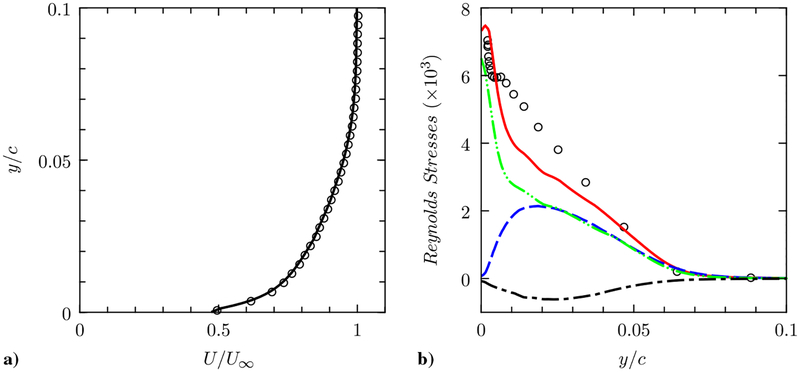
At the inflow plane located at x/c = −2.14, synthetic signals constructed with a digital filtering technique [46] are imposed to provide turbulent inflow data that match the experiment. This technique generates a sequence of random fluctuating signals that matches the target mean and covariance (the Reynolds stresses). Because only the mean and the streamwise turbulence intensity are available from the experiment, the missing Reynolds stress components were prescribed from the data from a boundary-layer LES [52] at a comparable Reynolds number. Figure 6 shows that the mean velocity at the inflow plane matches the experiment very well and that agreement of the streamwise intensity is acceptable. Figure 7 compares the mean velocity and the Reynolds stresses from the present WMLES at a downstream location before the hump (x/c = −0.81) to the data from a previously reported LES study [45]. Excellent agreement is observed. We therefore conclude that the inflow treatment in the present study closely reproduces the turbulence state in the experiment and that the inflow has evolved from random signals to realistic turbulence well before reaching the hump.

Fig. 6.

Profiles of a) mean streamwise velocity, and b) Reynolds stresses at the inflow plane (x/c = −2.14). Lines, present WMLES with the NEQWM; circles, experiment [42]. In Fig. 6b, red solid line, $\langle {u^{\prime }}^2\rangle /U_{\infty }^2$; green dash-dot-dotted line, $\langle {w^{\prime }}^2\rangle /U_{\infty }^2$; blue dashed line, $\langle {v^{\prime }}^2\rangle /U_{\infty }^2$; black dash-dotted line, $\langle u^{\prime }{v}^{\prime }\rangle /U_{\infty }^2$.

Fig. 7.

Profiles of a–b) mean streamwise velocity, and c) Reynolds stresses at a downstream location (x/c = −0.81). Lines, present WMLES with the NEQWM; squares, [45] (WMLES); in Fig. 7b, the dashed line represents the log law (U⁺ = 2.44 log y⁺ + 5.1). In Fig. 7c, red solid line, $\langle {u^{\prime }}^2\rangle /U_{\infty }^2$; green dash-dot-dotted line, $\langle {w^{\prime }}^2\rangle /U_{\infty }^2$; blue dashed line, $\langle {v^{\prime }}^2\rangle /U_{\infty }^2$; black dash-dotted line, $\langle u^{\prime }{v}^{\prime }\rangle /U_{\infty }^2$.

E. Cost of Wall Modeling

All simulations in the present study were carried out with 512 cores on the Pinto cluster, a modest-sized high-performance computing platform operated by Los Alamos National Laboratory. The cluster has 2464 CPU cores (Intel Xeon E5–2670 2.6 GHz) on 154 compute nodes (16 cores/node), with 32 GB/node memory and Qlogic InfiniBand Fat-Tree interconnect. All calculations took less than 50 wall-clock hours to advance 20 flow-through times c/U_∞. The average wall-clock times spent for integrating 10 simulation time steps were 1.6, 2.2, and 3.3 s for the no-slip LES (no wall model), the LES with the EQWM, and the LES with the NEQWM, respectively. The extra costs of wall modeling for the EQWM and the NEQWM are therefore about 40% and 100% of the standalone no-slip LES, respectively. The higher cost of the NEQWM is due to the matrix inversion associated with the fully implicit time integration. In general, the cost of wall modeling is a substantial fraction of the standalone LES. However, this cost should be deemed affordable because the grids employed in WMLES of high Reynolds number flows are already significantly coarser than the grids used for WRLES.

III. Results

A. Grid Convergence

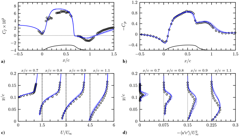
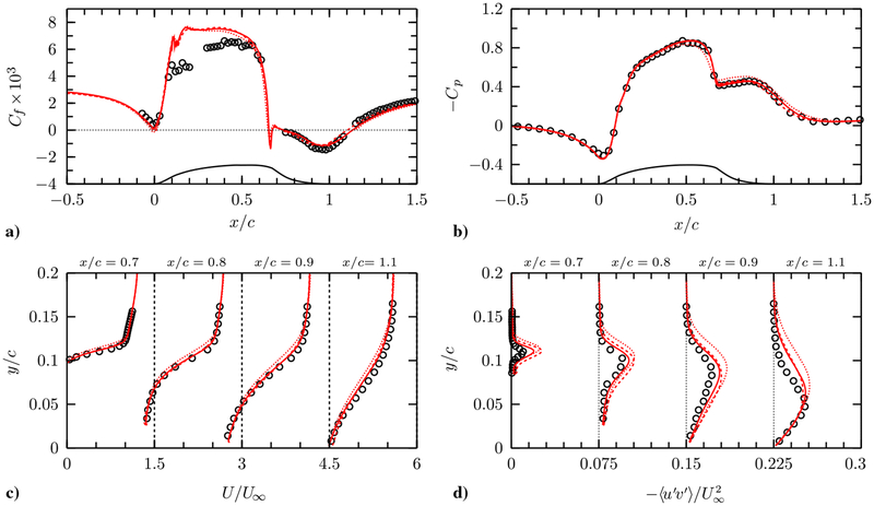
Figures 8 and 9 show the results obtained with the three grids described in Sec. II.C. LES with the NEQWM has mostly converged on the grid G2. A slower and less monotonic convergence is found with the EQWM in the separated region. Although the results obtained with the two wall models exhibit comparable degrees of agreement with the experiment, small but persistent outperformance of the NEQWM is observed in low-order statistics. The most notable difference is found in the skin friction distribution in the separation and recovery regions (x/c > 0.7). It is worth pointing out that C_f from the EQWM does not improve with the grid refinement, whereas C_f from the NEQWM obtained on the coarse grid is already in good agreement with the experiment.

Fig. 8.

Grid convergence of the LES + EQWM: coarse grid (G1), short-dashed line; medium grid (G2), long-dashed line; fine grid (G3), solid line: a) skin friction coefficient, b) wall-pressure coefficient, c) mean streamwise velocity, and d) Reynolds shear stress.

Fig. 9.

Grid convergence of the LES + NEQWM: coarse grid (G1), short-dashed line; medium grid (G2), long-dashed line; fine grid (G3), solid line: a) skin friction coefficient, b) wall-pressure coefficient, c) mean streamwise velocity, and d) Reynolds shear stress.

Although not shown for brevity, it was observed with the grids G2 and G3 that the mean velocity and wall-pressure distribution from the no-slip LES (no wall modeling) are only marginally worse than those from the wall-modeled calculations. The grids G2 and G3 are thus already approaching the wall-resolved limit where wall modeling is insignificant (also deducible from Fig. 5b), and the momentum loss evaluated with the no-slip condition is reasonably accurate. On the contrary, on the coarsest grid G1, the effect of wall modeling is evident, and performance of the two wall models is contrasted best. Because the main purpose of the present study is to contrast the wall-model performance in a practical condition of their deployment, the remainder of this paper will focus largely on delineating the results obtained with the coarse grid G1 unless stated otherwise.

B. Instantaneous Flow Field

Figure 10 visualizes the vortical structures present in the baseline grid (G1) calculations. In the no-slip LES, flow separation is apparently weaker than that found in the wall-modeled cases. Vortical structures are observed more sparsely than those found in the wall-modeled cases, especially in the separated region where large structures whose size is of the order of the shear-layer thickness are to be found predominantly.

Fig. 10.

Vortical structures identified by the isosurfaces of the second invariant of the velocity gradient tensor Q, colored with the streamwise velocity (G1 grid): a) no-slip LES (no wall model), b) LES with the NEQWM, and c) LES with the EQWM.

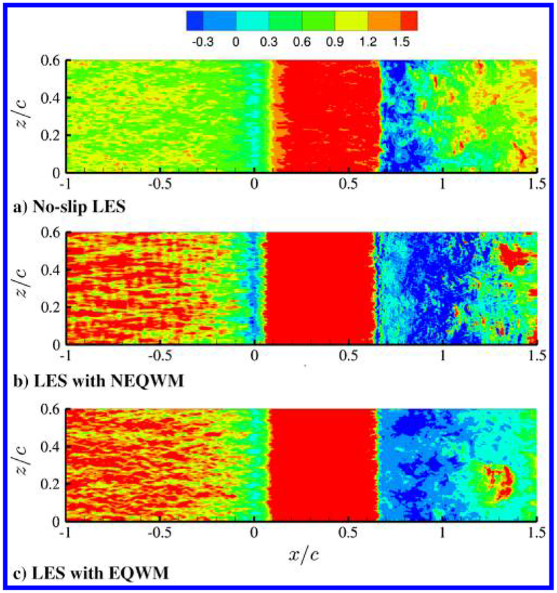
Figure 11 compares the instantaneous tangential wall-shear stress (τ_w) obtained from the same calculations. In WMLES, τ_w is obtained directly from the wall-model solution, whereas in the no-slip LES, it is the viscous flux evaluated with the LES velocity in the wall-adjacent control volumes and the zero-velocity condition on the wall. Apparently, τ_w in flat-plate portion (x/c < 0) from the no-slip LES is significantly underpredicted compared to that from WMLES. This is related to suppression of the stress-carrying motions and inherent underestimation of the viscous wall flux on a very coarse LES grid. Flow in the no-slip LES separates near the apex of the hump, but it has much weaker backflow and reattaches too early.

Fig. 11.

Contour of the instantaneous wall-tangential shear stress (G1 grid): a) no-slip LES (no wall model), b) LES with the NEQWM, and c)LES with the EQWM.

τ_w from the NEQWM and the EQWM are qualitatively similar, albeit with some difference. First, a weak separation near the leading edge of the hump is observed from the NEQWM, which is absent in the EQWM. Evidence of the leading-edge separation is not reported in the experiment, but it is observed in the resolved LES of [44]. Second, the backflow in the main separation region appears to be much stronger in the NEQWM than in the EQWM. Mean and fluctuations of τ_w after the reattachment are also higher in the NEQWM than in the EQWM. The trends in the NEQWM are in fact in better agreement with the experiment than those in the EQWM, as evidenced in Figs. 12 and 13.

Fig. 12.

a) Skin friction coefficient, and b) pressure coefficient along the bottom wall. Lines are from the present simulations run with the baseline grid (G1). Red dashed line, LES with the NEQWM; blue dashed-dotted line, LES with the EQWM; green solid line, no-slip LES; circles, experiment [42].

Fig. 13.

a) Tangential wall shear-stress fluctuations in the upstream flat-plate region, and b) wall-pressure fluctuations (${C^{\prime }}_p=2p_{w,\text{rms}}/\rho U_{\infty }^2$) near the hump. Lines are from the present simulations run with the baseline grid (G1). Red dashed line, LES with the NEQWM; blue dashed-dotted line, LES with the EQWM; green solid line, no-slip LES; circles, experiment [42].

C. Mean Flow and Turbulence Statistics

In this section, detailed flow statistics (including the mean velocity, Reynolds stresses, and mean forces exerted on the wall) from the (WM)LES calculations are compared to the experimental data and previous numerical studies. The separation bubble will be also characterized in terms of the separation and reattachment locations.

Figure 12a compares the skin friction coefficients $C_f=2{\tau }_w/\rho U_{\infty }^2$ from the present calculations to the measurement [42]. The no-slip LES data (no wall modeling) deviate significantly from the reference data, demonstrating that the LES grid is too coarse for direct application of the no-slip wall boundary condition. The use of wall models greatly improves the skin friction prediction. It is worth examining how the skin friction distribution differs in the two wall models because this alone accounts for the difference between the LES solutions obtained with different wall models (recall that LES uses the wall-shear stress boundary condition provided by the wall model). The difference in C_f is most pronounced in the separated and recovery regions. In these regions (x/c > 0.7), agreement with the experimental data is much better in the NEQWM than in the EQWM. In the pre-separation region on the hump (0 < x/c < 0.6), C_f from the NEQWM deviates from the experimental data slightly more than those from the EQWM, but this minor difference has a negligible influence on the mean velocity development up to the separation point (see Fig. 14). Last, little difference is found within the zero-pressure gradient flat-plate portion (x/c < −0.7), as expected.

Fig. 14.

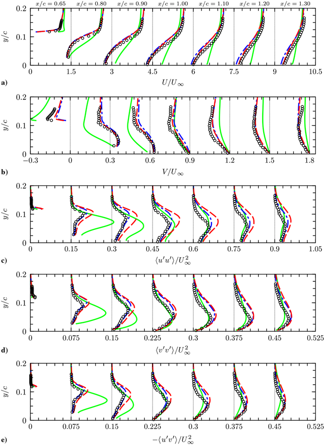
The mean velocity and Reynolds stress profiles from the present simulations run with the baseline grid (G1). Red dashed line, LES with the NEQWM; blue dashed-dotted line, LES with the EQWM; green solid line, no-slip LES; circles, experiment [42]. Profiles are shifted along the abscissa by multiples of 1.5, 0.3, 0.15, 0.075, and 0.075 for U, V, 〈u′ u′〉, 〈v′ v′〉, and 〈u′ v′〉, respectively.

Figure 12b shows the wall-pressure coefficients ($C_p=2\left(\langle p_w\rangle -p_{\infty }\right)/\rho U_{\infty }^2$). In the no-slip LES, flattening of C_p observed in the experiment at 0.6 < x/c < 1 has almost disappeared due to the too-weak separation. Additionally, the pressure minimum on the hump apex is significantly underpredicted due to the overly accelerated flow. The pressure coefficients from the WMLES are in good agreement with the experiment. C_p obtained with the NEQWM is slightly more accurate than that obtained with the EQWM in the separated and recovery regions (x/c > 0.9).

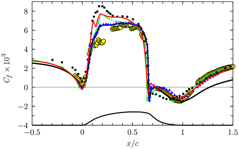
Figure 15 compares the present WMLES calculations to the previous numerical studies carried out with different turbulence modeling techniques and near-wall treatments, including two-dimensional (2-D) steady RANS with Spalart-Allmaras (SA) model [53], SA-based improved delayed DES (IDDES) [54], WMLES with an algebraic wall model [45], and resolved LES with no wall modeling [44]. Several observations can be made. All LES-based calculations (including the present study) produce a local peak in the skin friction in the hump forebody (x/c ≈ 0.2), which is absent in the experiment and the RANS-based calculations (steady RANS and IDDES). The 2-D RANS result, obtained with a grid resolution in the x–y plane (816 × 217) comparable to that of the grid G1, predicts a significantly delayed reattachment (RANS results obtained with more sophisticated two-equation and Reynolds-stress transport models also produced too large separation bubbles; see [53].) WMLES with an algebraic stress model performs reasonably well, but with notable deviation from the experiment in the upstream attached flow region as well as in the separation bubble. Among all simulations, the present WMLES with the NEQWM shows the best agreement with the resolved LES. Overall, the resolved LES, the present WMLES with the NEQWM, and the IDDES are equally in good agreement with the experiment in the separation and recovery regions. It is worth mentioning, however, that the IDDES results required deploying the new DES length-scale definition and calibrations proposed recently and that the widely used standard DES and delayed DES approaches failed catastrophically [54].

Fig. 15.

Skin friction predictions from the present and previous numerical studies. Red solid line, LES with the NEQWM (present study, grid G1); green dash-dot-dotted line, resolved LES [44]; black dash-triple-dotted line, 2-D RANS with Spalart-Allmaras one-equation model [53]; circles, experiment [42]; triangles, IDDES (Δ_sla-based, [54]); squares, WMLES [45] with Werner-Wengle wall model [19].

The wall shear-stress fluctuations from the WMLESs in the zero-pressure gradient region (Fig. 13a) are significantly lower than the value expected at this Reynolds number (${\tau }_{w,\text{rms}}^{+}\approx 0.42$) [55] (the experiment does not report the shear-stress fluctuations). On the contrary, the wall-pressure fluctuations from the WMLESs (Fig. 13b) are in good agreement with the experiment, consistent with the findings reported in [37].

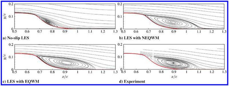
Figures 14a and 14b show the mean streamwise and vertical velocity profiles. Various streamwise locations from near the apex of the hump to the downstream of the reattachment point are considered (the flow reattaches at x/c = 1.1 in the experiment). The no-slip LES clearly yields poor mean velocity prediction on the grid G1. In the no-slip LES, the boundary layer on the hump carries too-high momentum due to the significantly underpredicted wall-shear stress. Consequently, the separation bubble is too small, and the flow reattaches too early (see Fig. 16). The velocity profiles after the reattachment are also grossly mispredicted with too high momenta. With wall modeling, prediction of the mean velocity improves substantially. In WMLES, the velocity profiles immediately before the separation (x/c = 0.65) are in close agreement with the experiment, implying that the attached flow on the hump is now better reproduced. The profiles in the separated and recovery regions are in reasonable agreement with the measurement. Consistent with the trend observed in the C_f prediction, the velocity predictions with the NEQWM are superior to those with the EQWM in the recovery region (x/c > 1). Prediction of the Reynolds stresses also improves significantly with wall modeling, especially in the separated region. Although the state-of-the-art RANS models tend to underpredict the maximum Reynolds shear stress by more than 50% [43], agreement of the present WMLES results with the experiment is satisfactory. For the Reynolds stresses, the EQWM prediction is more accurate than that of the NEQWM, although the difference is minor.

Fig. 16.

Averaged streamlines in the vicinity of the hump (baseline grid G1): a) no-slip LES, b) LES with the NEQWM, c) LES with the EQWM, and d) experiment [42].

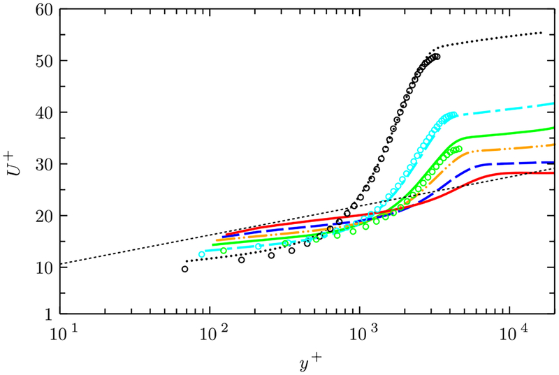
Figure 17 highlights the recovery of the perturbed boundary layer to an equilibrium boundary layer. Immediately after the reattachment (x/c = 1.2), the mean velocity profile resembles the laminar profile. The recovery is slow where the standard logarithmic layer has not fully recovered by x/c =2.2, corresponding to a downstream advection from the reattachment over a distance on the order of 1δ. The Reynolds number of the new equilibrium boundary layer is about Re_τ ≈ 10⁴, which is substantially higher than that of the upstream flat-plate flow (Re_τ ≈ 2000).

Fig. 17.

Mean streamwise velocity in wall units in the recovery (post-reattachment) region. Lines are from the LES with the NEQWM (grid G1) taken at x/c = 1.2, 1.3, 1.39, 1.5, 1.7, and 2.2 (top to bottom at y⁺ ≈ 10⁴). The straight dashed line denotes the log law (U⁺ = 2.44 log y⁺ + 5.1). Symbols are from the experiment [42].

Table 2 summarizes the separation bubble characteristics from all simulations carried out with different grid resolutions and wall boundary conditions. These include the separation and reattachment locations (identified with C_f = 0), the size of the separation bubble, and the percent error in the bubble length. Overall, LES with the two wall models predicts the reattachment location and the bubble length in close agreement with the experiment.

Table 2.

Separation bubble characteristics^a

Case	Separation xs/c	Reattachment xr/c	Bubble length (xr − xs)/c	Δ, %
Current LES (no-slip + G1)	0.690	0.855	0.165	−63
Current LES (NEQWM + G1)	0.65	1.135	0.485	9
Current LES (EQWM + G1)	0.672	1.138	0.466	5
Current LES (no-slip + G2)	0.649	1.032	0.383	− 14
Current LES (NEQWM + G2)	0.655	1.102	0.447	0.4
Current LES (EQWM + G2)	0.680	1.084	0.404	−9
Current LES (no-slip + G3)	0.656	1.096	0.440	− 1.1
Current LES (NEQWM + G3)	0.674	1.131	0.457	2.7
Current LES (EQWM + G3)	0.677	1.121	0.444	−0.2
[44] (WRLES)	0.641	1.09	0.449	1
[42] (experiment)	0.665(±0.005)	1.11(±0.003)	0.445	— —

^aNote that there is a ±2% uncertainty in the bubble length reported in the experiment.

D. Validity of the Equilibrium Wall Model

The source of underperformance of the EQWM in the separated and recovery regions is further analyzed by quantifying the nonequilibrium contributions neglected in the EQWM and by examining the validity of the constant-stress layer assumption. This would, in principle, require an a priori analysis of flow fields obtained with fully resolved simulations as in the work of [56], but such analysis is infeasible in the present study due to the high Reynolds number. Instead, our analysis is based on the NEQWM solution from the present study. This a posteriori analysis still has a practical value by elucidating how certain simplifying assumptions can manifest into the skin friction error in actual WMLES computations.

For this analysis, we use the incompressible form of the NEQWM equation. This is legitimate because the Mach number is less than 0.1, and the density variation is within 0.5% of the reference state in the domain of the NEQWM. The time and spanwise-averaged streamwise momentum equation in the NEQWM can be rearranged in the form of the EQWM as

$$\langle \frac{\partial }{\partial y}\left[\left(v+v_{t,wm}\right)\frac{\partial u}{\partial y}\right]\rangle =S_1$$ (2)

where the nonequilibrium source term S₁ in the right-hand side is defined as the sum of following terms (S₁= A₁ + P₁ − V₁):

$$\text{advection\hspace{0.17em}}{A}_1=\frac{\partial {\langle u\rangle }^2}{\partial x}+\frac{\partial \langle u\rangle \langle v\rangle }{\partial y}+\frac{\partial {\langle u^{\prime }\rangle }^2}{\partial x}+\frac{\partial \langle u^{\prime }{v}^{\prime }\rangle }{\partial y}$$ (3)

$$\text{pressure\hspace{0.17em}gradient\hspace{0.17em}}{P}_1=\frac{1}{\rho }\frac{\partial \langle P\rangle }{\partial x}$$ (4)

$$\text{lateral\hspace{0.17em}diffusion\hspace{0.17em}}{V}_1=\langle \frac{\partial }{\partial x}\left[\left(v+v_{t,wm}\right)\frac{\partial u}{\partial x}\right]\rangle$$ (5)

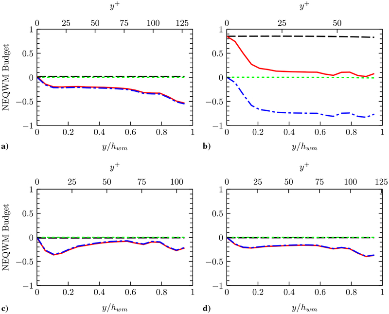
Figure 18 shows the profiles of the above NEQWM budget terms at four streamwise stations: at an attached region upstream of the hump (x/c = −0.8), within the separation bubble (x/c = 1), and in the recovery region (x/c =1.5 and 2). Note that the nonequilibrium contribution S₁ is nonzero everywhere. Streamwise diffusion is negligibly small in all regions, as expected. Pressure gradient is nearly constant along the wall-normal direction. In the attached regions, advection has the predominant contribution, and all other terms are negligible. At x/c = 2, the flow in the NEQWM has recovered from separation to exhibit a budget distribution similar to that in the upstream attached region. The characteristics in the separated region differ distinctly from those in the attached regions. Pressure gradient and advection have a significantly larger contribution throughout the inner portion of the separation bubble (x/c = 1). These terms largely balance each other, except in the close vicinity of the wall, where the advection vanishes due to the no-slip condition.

Fig. 18.

Budget of the mean streamwise momentum equation in the NEQWM as functions of the wall-normal distance normalized by the wall-model layer thickness h_wm and viscous wall unit v/u_τ. Blue dash-dotted line, advection A₁; black long dashed line, pressure gradient P₁; green short dashed line, lateral diffusion V₁; red solid line, total nonequilibrium source (S₁ = A₁ + P₁ – V₁): a)x/c = −0.8, b) x/c = 1, c)x/c = 1.5, and d)x/c = 2. The budget terms are normalized with the hump chord c and the freestream velocity U_∞.

Based on the budget analysis, it can now be further deduced how the wall-shear stress in the NEQWM would change by omitting the nonequilibrium contribution S₁, as is done in the EQWM. Integrating Eq. (2) at a fixed streamwise location in the vertical direction (from the wall to the matching location), the following expression for the wall-shear stress in the NEQWM is obtained:

$${\tau }_w={\langle \left(\mu +{\mu }_{t,wm}\right)\frac{\partial u}{\partial y}\rangle }_{y=h_{wm}}+\rho {\int }_0^{h_{wm}}-S_1\left(y\right)\text{d}y$$ (6)

From Fig. 18, the second term in Eq. (6) has positive and negative contributions to τ_w in the attached and separated regions, respectively. Therefore, neglecting S₁(i.e., EQWM) would result in under- and overprediction of τ_w in the attached and separated regions, respectively. This result is consistent with the trend of the skin friction from the EQWM, compared to that from the NEQWM (for instance, see Fig. 12a at x/c = 1 and 1.5).

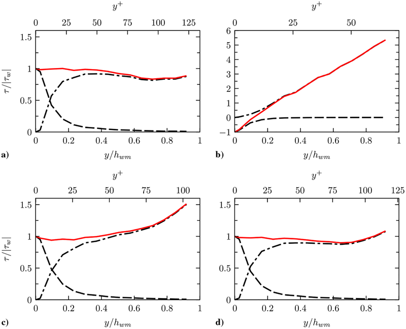
The validity of the EQWM assumption can be also assessed through the profiles of the total shear stress from the NEQWM. Recall that the EQWM by construction assumes that the sum of the viscous and turbulent shear stresses is constant along the wall-normal direction. Figure 19 shows the profiles of the shear stresses at the same streamwise stations as those considered in Fig. 18. As expected, the equilibrium assumption seems reasonable in the upstream attached region (x/c = −0.8) and in the recovery region far downstream of the reattachment point (x/c = 2). However, the constant total stress assumption ceases to hold within the separation bubble and close to the reattachment, where considerable total stress gradients are found.

Fig. 19.

Profiles of the shear stresses in the NEQWM as functions of the wall-normal distance normalized by the wall-model thickness h_wm and viscous wall unit v/u_τ. Dashed line, viscous shear stress(〈μ(∂u/∂y)〉); dash dotted line, turbulent shear stress (〈μ_t,wm(∂u/∂y)〉 − 〈u′ v′〉); red solid line, total shear stress (viscous + turbulent): a) x/c = −0.8, b) x/c = 1, c) x/c = 1.5, and d) x/c = 2.

IV. Conclusions

Large-eddy simulations with two wall-modeling techniques have been applied to a separated and reattaching flow over the NASA wall-mounted hump. It was shown that WMLES predicts the mean and turbulence statistics reasonably well on a coarse grid where the no-slip LES fails. The more elaborate and costly nonequilibrium model outperformed the equilibrium model, especially in predicting the mean velocity and mean forces exerted on the wall (skin friction and wall-pressure coefficients) in the separated and recovery regions. The source of the EQWM’s underperfoimance in the separation and recovery regions was traced back to the invalidity of the equilibrium assumption in these regions. It was shown quantitatively that the assumptions of the constant-stress layer and negligible nonequilibrium effects are largely invalid in these regions, leading to the erroneous skin friction predictions. Wall modeling significantly improved the prediction of wall-pressure fluctuations in the separated region, whereas wall shear-stress fluctuations modeled entirely through the wall models appear to be significantly underpredicted.

Nomenclature

C_f

skin friction coefficient

C_p

wall-pressure coefficient

c

hump chord length, m

M

Mach number

P

pressure, kg/(m • s²)

Re

Reynolds number

T

temperature, K

U, V, W

mean velocity in x, y, and z directions, m/s

u_τ

friction velocity, m/s

x, y, z

coordinates in the streamwise, vertical, and spanwise directions, m

δ

99% boundary-layer thickness, m

μ

dynamic viscosity, kg/(m • s)

v

kinematic viscosity, m²/s

ρ

density, kg/m³

τ_w

wall-tangential shear stress, Pa

Subscripts

w

quantity defined on the wall

∞

reference state at the inlet freestream

Superscripts

′

fluctuation with respect to the mean

+

quantity in wall unit (nondimensionalized with ν and u_τ)

References

- [1].Skote M, and Henningson DS, “Direct Numerical Simulation of a Separated Turbulent Boundary Layer,” Journal of Fluid Mechanics, Vol. 471, November 2002, pp. 107–136. doi: 10.1017/S0022112002002173 [DOI] [Google Scholar]
- [2].Germano M, Piomelli U, Moin P, and Cabot WH, “A Dynamic Subgrid-Scale Eddy-Viscosity Model,” Physics of Fluids A, Vol. 3, No. 7, 1991, pp. 1760–1765. doi: 10.1063/1.857955 [DOI] [Google Scholar]
- [3].Lilly DK, “A Proposed Modification of the Germano Subgrid-Scale Closure Method,” Physics of Fluids A, Vol.4, No. 3, 1992, pp. 633–635. doi: 10.1063/1.858280 [DOI] [Google Scholar]
- [4].Moin P, Squires K, Cabot W, and Lee S, “A Dynamic Subgrid-Scale Model for Compressible Turbulence and Scalar Transport,” Physics of Fluids, Vol. 3, No. 11, 1991, pp. 2746–2757. doi: 10.1063/1.858164 [DOI] [Google Scholar]
- [5].Mittal R, and Moin P, “Suitability of Upwind-Biased Finite Difference Schemes for Large-Eddy Simulation of Turbulent Flows,” AIAA Journal, Vol. 35, No. 8, 1997, pp. 1415–1417. doi: 10.2514/2.253 [DOI] [Google Scholar]
- [6].Kravchenko AG, and Moin P, “Numerical Studies of Flow over a Circular Cylinder at ReD = 3900,” Physics of Fluids, Vol. 12, No. 2, 2000, pp. 403–417. doi: 10.1063/1.870318 [DOI] [Google Scholar]
- [7].You D, and Moin P, “A Dynamic Global-Coefficient Subgrid-Scale Eddy-Viscosity Model for Large-Eddy Simulation in Complex Geometries,” Physics of Fluids, Vol. 19, No. 6, 2007, Paper 065110. [Google Scholar]
- [8].You D, Ham F, and Moin P, “Discrete Conservation Principles in Large-Eddy Simulation with Application to Separation Control over an Airfoil,” Physics of Fluids, Vol. 20, No. 10, 2008, Paper 101515. doi: 10.1063/1.3006077 [DOI] [Google Scholar]
- [9].Verma A, and Mahesh K, “A Lagrangian Subgrid-Scale Model with Dynamic Estimation of Lagrangian Time Scale for Large Eddy Simulation of Complex Flows,” Physics of Fluids, Vol. 24, No. 8, 2012, Paper 085101. doi: 10.1063/1.4737656 [DOI] [Google Scholar]
- [10].Fröhlich J, Mellen CP, Rodi W, Temmerman L, and Leschziner MA, “Highly Resolved Large-Eddy Simulation of Separated Flow in a Channel with Streamwise Periodic Constrictions,” Journal of Fluid Mechanics, Vol. 526, March 2005, pp. 19–66. doi: 10.1017/S0022112004002812 [DOI] [Google Scholar]
- [11].Bose ST, “Explicitly Filtered Large-Eddy Simulation: With Application to Grid Adaptation and Wall Modeling,” Ph.D. Dissertation, Stanford Univ., Stanford, CA, 2012. [Google Scholar]
- [12].Jiménez J, and Moser RD, “Large-Eddy Simulations: Where Are We and What Can We Expect?” AIAA Journal, Vol. 38, No. 4, April 2000, pp.605–612. doi: 10.2514/3.14451 [DOI] [Google Scholar]
- [13].Sayadi T, and Moin P, “Large Eddy Simulation of Controlled Transition to Turbulence,” Physics of Fluids, Vol. 24, No. 11, 2012, Paper 114103. [Google Scholar]
- [14].Choi H, and Moin P, “Grid-Point Requirements for Large Eddy Simulation: Chapman’s Estimates Revisited,” Physics of Fluids, Vol. 24, No. 1, 2012, Paper 011702. [Google Scholar]
- [15].Slotnick J, Khodadoust A, Alonso J, Darmofal D, Gropp W, Lurie E, and Mavriplis D, “CFD Vision 2030 Study: A Path to Revolutionary Computational Aerosciences,” NASA CR-2014–218178, 2014. [Google Scholar]
- [16].Deardorff JW, “The Numerical Study of Three Dimensional Turbulent Channel Flow at Large Reynolds Numbers,” Journal of Fluid Mechanics, Vol. 41, No. 2, 1970, pp. 453–480. doi: 10.1017/S0022112070000691 [DOI] [Google Scholar]
- [17].Schumann U, “Subgrid Scale Model for Finite Difference Simulations of Turbulent Flows in Plane Channels and Annuli,” Journal of Computational Physics, Vol. 18, No. 4, 1975, pp. 376–404. doi: 10.1016/0021-9991(75)90093-5 [DOI] [Google Scholar]
- [18].Piomelli U, Ferziger J, Moin P, and Kim J, “New Approximate Boundary Conditions for Large Eddy Simulations of Wall-Bounded Flows,” Physics of Fluids A, Vol. 1, No. 6, 1989, pp. 1061–1068. doi: 10.1063/1.857397 [DOI] [Google Scholar]
- [19].Werner H, and Wengle H, “Large-Eddy Simulation of Turbulent Flow over and Around a Cube in a Plate Channel,” Turbulent Shear Flows, Vol. 8, Springer, Berlin, 1993, pp. 155–168. [Google Scholar]
- [20].Balaras E, Benoccis C, and Piomelli U, “Two-Layer Approximate Boundary Conditions for Large-Eddy Simulations,” AIAA Journal, Vol. 34, No. 6, 1996, pp. 1111–1119. doi: 10.2514/3.13200 [DOI] [Google Scholar]
- [21].Cabot W, and Moin P, “Approximate Wall Boundary Conditions in Large-Eddy Simulation of High Reynolds Number Flow,” Flow, Turbulence and Combustion, Vol. 63, Nos. 1–4, 2000, pp. 269–291. doi: 10.1023/A:1009958917113 [DOI] [Google Scholar]
- [22].Wang M, and Moin P, “Dynamic Wall Modeling for Large-Eddy Simulation of Complex Turbulent Flows,” Physics of Fluids, Vol. 14, No. 7, 2002, pp. 2043–2051. doi: 10.1063/1.1476668 [DOI] [Google Scholar]
- [23].Park GI, and Moin P, “An Improved Dynamic Non-Equilibrium Wall-Model for Large Eddy Simulation,” Physics of Fluids, Vol. 26, No. 1, 2014, Paper 015108. doi: 10.1063/1.4861069 [DOI] [Google Scholar]
- [24].Kawai S, and Larsson J, “Dynamic Non-Equilibrium Wall-Modeling for Large Eddy Simulation at High Reynolds Numbers,” Physics of Fluids, Vol. 25, No. 1, 2013, Paper 015105. doi: 10.1063/1.4775363 [DOI] [Google Scholar]
- [25].Yang XIA, Sadique J, Mittal R, and Meneveau C, “Integral Wall Model for Large Eddy Simulations of Wall-Bounded Turbulent Flows,” Physics of Fluids, Vol. 27, No. 2, 2015, Paper 025112. [Google Scholar]
- [26].Chung D, and Pullin DI, “Large-Eddy Simulation and Wall Modelling of Turbulent Channel Flow,” Journal of Fluid Mechanics, Vol. 631, July 2009, pp. 281–309. doi: 10.1017/S0022112009006867 [DOI] [Google Scholar]
- [27].Cheng W, Pullin DI, and Samtaney R, “Large-Eddy Simulation of Separation and Reattachment of Flat Plate Turbulent Boundary Layer,” Journal of Fluid Mechanics, Vol. 785, December 2015, pp. 78–108. doi: 10.1017/jfm.2015.604 [DOI] [Google Scholar]
- [28].Bose ST, and Moin P, “A Dynamic Slip Boundary Condition for Wall-Modeled Large-Eddy Simulation,” Physics of Fluids, Vol. 26, No. 1, 2014, Paper 015104. doi: 10.1063/1.484953 [DOI] [Google Scholar]
- [29].Spalart PR, “Detached-Eddy Simulation,” Annual Review of Fluid Mechanics, Vol. 41, 2009, pp. 181–202. doi: 10.1146/annurev.fluid.010908.165130 [DOI] [Google Scholar]
- [30].Piomelli U, Rouhi A, and Geurts BJ, “A Grid-Independent Length Scale for Large-Eddy Simulations,” Journal of Fluid Mechanics, Vol. 766, March 2015, pp. 499–527. doi: 10.1017/jfm.2015.29 [DOI] [Google Scholar]
- [31].Rouhi A, Piomelli U, and Geurts B, “Dynamic Subfilter-Scale Stress Model for Large-Eddy Simulations,” Physical Review Fluids, Vol. 1, No. 4, 2016, Paper 044401. doi: 10.1103/PhysRevFluids.1.044401 [DOI] [Google Scholar]
- [32].Balakumar P, Park GI, and Pierce B, “DNS, LES, and Wall-Modeled LES of Separating Flow over Periodic Hills,” Proceedings of the Summer Program 2014, Center for Turbulence Research, Stanford Univ., Stanford, CA, 2014, pp. 407–415. [Google Scholar]
- [33].Bodart J, Larsson J, and Moin P, “Large Eddy Simulation of High-Lift Devices,” 21st AIAA Computational Fluid Dynamics Conference, AIAA Paper 2013–2724, 2013. [Google Scholar]
- [34].Bermejo-Moreno I, Campo L, Larsson J, Bodart J, Helmer D, and Eaton JK, “Confinement Effects in Shock Wave/Turbulent Boundary Layer Interactions Through Wall-Modelled Large-Eddy Simulations,” Journal of Fluid Mechanics, Vol. 758, November 2014, pp. 5–62. doi: 10.1017/jfm.2014.505 [DOI] [Google Scholar]
- [35].Park GI, and Moin P, “Numerical Aspects and Implementation of a Two-Layer Zonal Wall Model for LES of Compressible Turbulent Flows on Unstructured Meshes,” Journal of Computational Physics, Vol. 305, January 2016, pp. 589–603. doi: 10.1016/j.jcp.2015.11.010 [DOI] [Google Scholar]
- [36].Toro E, Spruce M, and Speares W, “Restoration of the Contact Surface in the HLL-Riemann Solver,” Shock Waves, Vol. 4, No. 1, 1994, pp.25–34. doi: 10.1007/BF01414629 [DOI] [Google Scholar]
- [37].Park GI, and Moin P, “Space-Time Characteristics of Wall-Pressure and Wall Shear-Stress Fluctuations in Wall-Modeled Large Eddy Simulation,” Physical Review Fluids, Vol. 1, No. 2, 2016, Paper 024404. doi: 10.1103/PhysRevFluids.1.024404 [DOI] [PMC free article] [PubMed] [Google Scholar]
- [38].Bodart J, and Larsson J, “Wall-Modeled Large Eddy Simulation in Complex Geometries with Application to High-Lift Devices,” Annual Research Briefs 2011, Center for Turbulence Research, Stanford Univ., Stanford, CA, 2011, pp. 37–48. [Google Scholar]
- [39].Piomelli U, and Balaras E, “Wall-Layer Models for Large-Eddy Simulations,” Annual Review of Fluid Mechanics, Vol. 34, 2002, pp.349–374. doi: 10.1146/annurev.fluid.34.082901.144919 [DOI] [Google Scholar]
- [40].Degraaff DB, and Eaton JK, “Reynolds-Number Scaling of the Flat-Plate Turbulent Boundary Layer,” Journal of Fluid Mechanics, Vol. 422, 2000, pp. 319–346. doi: 10.1017/S0022112000001713 [DOI] [Google Scholar]
- [41].Kawai S, and Larsson J, “Wall-Modeling in Large Eddy Simulation: Length Scales, Grid Resolution, and Accuracy,” Physics of Fluids, Vol. 24, No. 1, 2012, Paper 015015. doi: 10.1063/1.3678331 [DOI] [Google Scholar]
- [42].Greenblatt D, Paschal KB, Yao CS, Harris J, Schaeffler NW, and Washburn AE, “A Separation Control CFD Validation Test Case, Part 1: Baseline and Steady Suction,” 2nd AIAA Flow Control Conference, AIAA Paper 2004–2220, June-July 2004. [Google Scholar]
- [43].Rumsey CL, Gatski TB, Sellers WL III, Vasta VN, and Viken A, “Summary of the 2004 Computational Fluid Dynamics Validation Workshop on Synthetic lets,” AIAA Journal, Vol. 44, No. 2, 2006, pp. 194–207. doi: 10.2514/1.12957 [DOI] [Google Scholar]
- [44].You D, Wang M, and Moin P, “Large-Eddy Simulation of Flow over a Wall-Mounted Hump with Separation Control,” AIAA Journal, Vol. 44, No. 11, 2006, pp. 2571–2577. doi: 10.2514/1.21989 [DOI] [Google Scholar]
- [45].Avdis A, Lardeau S, and Leschziner M, “Large Eddy Simulation of Separated Flow over a Two-Dimensional Hump with and Without Control by Means of a Synthetic Slot-Jet,” Flow, Turbulence and Combustion, Vol. 83, No. 3, 2009, pp. 343–370. doi: 10.1007/s10494-009-9218-y [DOI] [Google Scholar]
- [46].Klein M, Sadiki A, and Janicka J, “A Digital Filter Based Generation of Inflow Data for Spatially Developing Direct Numerical or Large Eddy Simulations,” Journal of Computational Physics, Vol. 186, No. 2, 2003, pp.652–665. doi: 10.1016/S0021-9991(03)00090-1 [DOI] [Google Scholar]
- [47].Lund TS, Wu X, and Squires KD, “Generation of Turbulent Inflow Data for Spatially-Developing Boundary Layer Simulations,” Journal of Computational Physics, Vol. 140, No. 2, 1998, pp. 233–258. doi: 10.1006/jcph.1998.5882 [DOI] [Google Scholar]
- [48].Chapman DR, “Computational Aerodynamics Development and Outlook,” AIAA Journal, Vol. 17, No. 12, 1979, pp. 1293–1313. doi: 10.2514/3.61311 [DOI] [Google Scholar]
- [49].Iyer PS, Park GI, and Malik MR, “A Comparative Study of Wall Models for LES of Turbulent Separated Flow,” Proceedings of the Summer Program 2016, Center for Turbulence Research, Stanford Univ., Stanford, CA, 2016, pp. 325–334. [Google Scholar]
- [50].Bodart J, and Larsson J, “Sensor-Based Computation of Transitional Flows Using Wall-Modeled Large Eddy Simulation,” Annual Research Briefs 2012, Center for Turbulence Research, Stanford Univ., Stanford, CA, 2012, pp. 229–240. [Google Scholar]
- [51].Poinsot TJ, and Lele SK, “Boundary Conditions for Direct Simulations of Compressible Viscous Flows,” Journal of Computational Physics, Vol. 101, No. 1, 1992, pp. 104–129. doi: 10.1016/0021-9991(92)90046-2 [DOI] [Google Scholar]
- [52].Schlatter P, Li Q, Brethouwer G, Johansson AV, and Henningson DS, “Simulations of Spatially Evolving Turbulent Boundary Layers up to Reθ = 4300,” International Journal of Heat and Fluid Flow, Vol. 31, No. 3, 2010, pp. 251–261. doi: 10.1016/j.ijheatfluidflow.2009.12.011 [DOI] [Google Scholar]
- [53].Rumsey CL, “NASA Langley Research Center Turbulence Modeling Resource,” NASA Langley Research Center, Hampton, VA, https://turbmodels.larc.nasa.gov/nasahump_val_sa.html [retrieved Sept. 2016]. [Google Scholar]
- [54].Guseva EK, Garbaruk AV, and Strelets MK, “Assessment of Delayed DES and Improved Delayed DES Combined with a Shear-Layer-Adapted Subgrid Length-Scale in Separated Flows,” Flow, Turbulence and Combustion, Vol. 98, No. 2, 2017, pp. 481–502. doi: 10.1007/s10494-016-9769-7 [DOI] [Google Scholar]
- [55].Mathis R, Marusic I, Chernyshenko S, and Hutchins N, “Estimating Wall-Shear-Stress Huctuations Given an Outer Region Input,” Journal of Fluid Mechanics, Vol. 715, January 2013, pp. 163–180. doi: 10.1017/jfm.2012.508 [DOI] [Google Scholar]
- [56].Hickel S, Touber E, Bodart J, and Larsson J, “A Parametrized Non-Equilibrium Wall-Model for Large-Eddy Simulations,” Proceedings of the Summer Program 2012, Center for Turbulence Research, Stanford Univ., Stanford, CA, 2012, pp. 229–240. [Google Scholar]