An Investigation of CNN Models for Differentiating Malignant from Benign Lesions Using Small Pathologically Proven Datasets

Abstract

Cancer has been one of the most threatening diseases to human health. There have been many efforts devoted to the advancement of radiology and transformative tools (e.g. non-invasive computed tomographic or CT imaging) to detect cancer in early stages. One of the major goals is to identify malignant from benign lesions. In recent years, machine deep learning (DL), e.g. convolutional neural network (CNN), has shown encouraging classification performance on medical images. However, DL algorithms always need large datasets with ground truth. Yet in the medical imaging field, especially for cancer imaging, it is difficult to collect such large volume of images with pathological information. Therefore, strategies are needed to learn effectively from small datasets via CNN models. To forward that goal, this paper explores two CNN models by focusing extensively on expansion of training samples from two small pathologically proven datasets (colorectal polyp dataset and lung nodule dataset) and then differentiating malignant from benign lesions. Experimental outcomes indicate that even in very small datasets of less than 70 subjects, malignance can be successfully differentiated from benign via the proposed CNN models, the average AUCs (area under the receiver operating curve) of differentiating colorectal polyps and pulmonary nodules are 0.86 and 0.71, respectively. Our experiments further demonstrate that for these two small datasets, instead of only studying the original raw CT images, feeding additional image features, such as the local binary pattern of the lesions, into the CNN models can significantly improve classification performance. In addition, we find that our explored voxel level CNN model has better performance when facing the small and unbalanced datasets.

1. Introduction

As reported from World Health Organization (WHO), cancer is the second leading cause of death globally, and is responsible for an estimated 9.6 million deaths in 2018 (WHO, 2018). Globally, about 1 in 6 deaths is due to cancer (WHO, 2018). Lung and colorectal cancers are the most common strains of cancer, resulting in around 2.09 and 1.80 million deaths in the year of 2018 (WHO, 2018). In recent years, efforts have been devoted to the advancement of radiology and transformative tools (e.g. non-invasive computed tomographic or CT imaging) to detect and diagnose cancers in the early stage, which would significantly increase the survival rates of cancer patients (Forstner et al., 1995; Gurney, 1996; Bipat et al., 2004; Chen et al., 2004; International Early Lung Cancer Action Program Investigators, 2006; Doi, 2007; Frangioni, 2008; Popovtzer et al., 2008). While the early detection rate has significantly increased, the false positive (FP) detection rate has also increased significantly, rendering a challenging task for reducing the FP rate for the diagnosis or true detection, particular for the differentiation of malignance from benign detections (Wang et al., 2008; Jayasurya et al., 2010; Sun et al., 2013; Zięba et al., 2014). This differentiation or classification problem is most related to the machine learning (ML) filed, where a learning algorithm is trained firstly to learn from a dataset (which includes some identifiable labels) to identify some patterns and make relevant decisions corresponding to identifiable labels and then the learning algorithm is expect to perform well for a desired task, for example differentiating malignant from benign lesions. Despite great progress in the ML field, better classification algorithms are always desired to achieve better classification performance. A good classification algorithm is extremely desirable for cancer diagnosis because of limited datasets with pathologically proven ground truth available for the training (Ciompi et al., 2015; Hua et al., 2015; Rouhi et al., 2015; Shen et al., 2015; Ribeiro et al., 2016; Sun et al., 2016; Zhang et al., 2017; Shen et al., 2017).

In recent years, machine deep learning (DL) algorithm based artificial intelligence (AI) has been a hot trend to assist experts to ease the burden of their jobs with reasonably good or better performance in all fields (Ngiam et al., 2011; Mnih et al., 2013; Deng and Yu, 2014; Schmidhuber, 2015; LeCun et al., 2015). DL algorithms, e.g. convolutional neural network (CNN), have shown encouraging classification performance on medical images (Lo et al., 1995; Sahiner et al., 1996; Li et al., 2014; Milletari et al., 2016; Liu et al., 2018; Zhang et al., 2018). Compared with traditional ML/pattern recognition algorithms, the major advantage of CNN is that the CNN architectural model can autonomously learn to extract high-level features to pursue the best classification performance. Instead of designing the handcrafted features for classification, CNN designs proper models to learn distinguishable features from input data, yield the corresponding optimal classification results, and achieve a good generalization performance for the prediction. It is worth noting that, due to the huge number of parameters that need to be trained for the designed model, DL algorithms always need large datasets to satisfactorily train the model and obtain meaningful features for better performance. For example, the ImageNet is a widely used and growing image dataset with around 14,197,122 labeled images (Deng et al., 2009). In the medical imaging field, especially in the cancer imaging area, it is very difficult and extremely expensive to collect large number of images from patients with pathologically proven ground truth. Therefore, the available datasets are always small in volume.

To effectively learn from small medical imaging datasets via CNN models, some reports focus on expanding the training dataset volume (Dellana and Roy, 2016; Wong et al., 2016; Wigington et al., 2017; Salamon and Bello, 2017; Yedroudj et al., 2018). For example, a new concept called “transfer learning” uses huge datasets like ImageNet with natural images to initialize and optimize the weights of the model, then to fine the weights by using the medical images (Van Opbroek et al., 2015; Tajbakhsh et al., 2016; Shin et al., 2016). However, whether natural images have the similar patterns as the medical images are under debated, especially when the medical images are quite unique (like CT images), thus this option is interesting but lacks fundamental understanding between natural images and medical images. Another example is expanding the medical images at multi-scale, which means cutting the original raw images into patches at different level of field of vision (Shen et al., 2015; Keuper et al., 2016; Quan et al., 2016). This way can significantly improve the size of the training dataset based on the original medical images, however, some challenges will be encountered, e.g. how to assign the labels to those patches when some patches only contain a few polyp/nodule tissues, will those patches affect the performance, etc.? Thus, how to study small dataset via CNN models is still a tough challenge.

For the purpose of relieving the challenges in the medical applications of small pathologically proven datasets, we proposed two CNN models to investigate their learning capability and classification performance between malignant and benign polyps/nodules. The first model is multi-channel-multi-slice two-dimensional CNN model (MCMS-2D CNN). The advantage of the MCMS-2D CNN model is that expanding the training datasets offers an opportunity to (1) use multi-channel strategy to include all kinds of feature maps available, like the original raw images, the local binary pattern (LBP) maps (to include the texture information), the histogram of gradient (HOG) maps and the gradient of images (to include the edge information), and (2) learn abstract features from multi-slice images of each polyp/nodule volume. It is worth noting that pathologically proven datasets are always small and unbalanced. To better deal with unbalanced datasets, we designed the second CNN model, which is voxel-level one-dimensional CNN model (V-1D CNN). The advantage of V-1D CNN is that the training datasets can be expanded significantly by treating the inputs at the image voxel level (the number of voxels can be very large even though the dataset is small). For example, one polyp/nodule volume may contain hundreds of image voxels, thus using voxel level inputs will significantly expanding the training datasets. By this simple, innovative idea, we will learn and predict each voxel in the training stage. And after gather all the information from voxels, we would expect to have an improved model to label each polyp/nodule as either malignant or benign. We agree that when we generate inputs at voxel level, noises will be inevitability produced into the training datasets. However, it is a tradeoff problem, the benefits are more training samples and their local information can be used to improve the classification performance.

The rest of the paper is designed as follows: in the Method section, we will present the above-mentioned two pathologically proven datasets of polyps and nodules and describe the proposed two CNN models. In the Results section, we will show the classification performance of these two CNN models and report quantitative measures on the classification performance. In the Discussion and Conclusion section, we will summarize the major contributions and outline the weaknesses of the proposed two CNN models for our future research interest to overcome them.

2. Method

In this study, we proposed two CNN models to study the classifier to differentiate malignant from benign nodules/polyps on small datasets. The proposed pipeline is consisting of four major steps: (1) extracting and generating the inputs for the CNN models; (2) designing the CNN models to study the differences between malignant and benign; (3) adopting the validation approach to evaluate the performance of the model we learned; and (4) studying the performance of the model via statistical analysis.

2.1. Datasets and Inputs of CNN Models

As we know, most publicly available cancer image datasets are not pathologically proven, e.g. a very commonly used dataset: LIDC-IDRI (Armato et al., 2011). Although many studies have used non-pathologically proven datasets and achieved very good classification performance to differentiate malignant from benign lesions, without the ground truth for the labels to confirm their classification performance, their clinical impacts are limited. For example, Litjens et al. (2017) mentioned that for many nodules in the LIDC dataset, the experts have different opinions and different labels (marked lesions belonging to one of three categories (“nodule > or =3 mm,” “nodule <3 mm,” and “non-nodule > or =3 mm”), thus bias will be inevitable included for the labelling, which is called “label noise”. Another example is shown in Han et al. (2015), they mentioned that according to the rules of constructing the LIDC-IDRI database, the malignancy assessments are defined in five levels, i.e., 1, 2, 3, 4, and 5, from benign to malignant. Since group “3” means the malignancy of the corresponding nodule is uncertain, thus the nodules with label “3” could be treated in two different ways in the study, i.e. either “3” belongs to benign class or “3” belongs to malignant class. It is interested to see that the classification performances of the two ways are largely different (one is about 0.91 AUC, another one is about 0.78 AUC). Thus, further experiments on pathologically proven datasets are needed. As one major motivation of this study, two small pathologically proven datasets were used to evaluate our CNN models. The data information is listed in Table 1. The sample sizes of the two pathologically proven datasets are relatively small (both N <70). Specifically, the lung nodule dataset is quite unbalanced (73% malignant). For our pathologically proven datasets, experts went through the 3D CTC images slice by slice and identified the suspicious region of interest (ROI), then drawn the boundaries, so these two datasets are clinically meaningful.

Table 1.

Two pathologically proven small datasets.

Dataset	Malignant N (%)	Benign N (%)	Total	Pathological Report
Colorectal Polyps	32 (51%)	31 (49%)	63	Yes
Lung Nodules	49 (73%)	18 (27%)	67	Yes

Dataset 1:

The patient, who was scheduled for CT scan at University of Wisconsin, USA, was recruited to this study under informed consent after approval by the Institutional Review Board. Tube voltage is 120 kVp and dose is followed by automatic exposure control. A total of 59 patients with 63 polyp masses, including 31 benign and 32 malignant. In the category of benign, four sub-categories are recorded from the pathology reports, they are Serrated Adenoma (3 cases), Tubular Adenoma (2 cases), Tubulovillous Adenoma (21 cases), Villous Adenoma (5 cases). In the category of malignant, it is Adenocarcinoma only (32 cases). In total, 51% are males and 49% are females. The patient age ranges from 45.9 to 91.6 years old (mean age of 66.5 years old). The size of the polyp masses ranges from 3 to 8 cm (mean of 4.2cm). The patients were scanned by a routine clinical non-contrast CT scanning protocol covering the entire abdomen volume. Each abdominal CT image volume consists of more than 400 image slices, each image slice has an array size of 512×512, and each image element or voxel is nearly cubic with edge size of 1mm. Contour of each polyp image slice inside the CT abdominal image volume was drawn by experts on a slice-by-slice manner using a semi-automated segmentation algorithm. Because of a relatively large polyp size, every drawn polyp contour can be allocated into an image array size of 48×48. Depending on the size of the polyp volume, the number of the 48×48 image slices can vary from 17 to 103. The routing CT scan, the drawn polyp borders, and the pathological labels of each polyp were inputted for the proposed CNN-based machine learning pipeline for polyp classification.

Dataset 2:

The patient, who was scheduled for CT-guided lung nodule needle biopsy at Stony Brook University Hospital, USA, was recruited to this study under informed consent after approval by the Institutional Review Board. Tube voltage is 120 kVp and dose is followed by automatic exposure control. A total of 66 patients with 67 lung nodules, including 18 benign and 49 malignant. The average age of the patients is 69.5 years old, ranging from 33 to 91 years old, and 52% of the patients are males and 48% are females. The diameter of these nodules ranges from 0.91 to 13.08 cm (mean size of 3.15 cm). Each patient underwent a routine clinical non-contrast CT scanning protocol covering nearly the entire chest volume, resulting in more than 200 image slices of 512×512 array size, and each image voxel is nearly cubic with edge size of 1mm. The border of each nodule image slice inside the routine patient CT scan was drawn by experts on a slice-by-slice manner using a semi-automated segmentation algorithm. All the drawn nodule image slices can be allocated into an image array size of 32×32. Depending on the size of the nodule volume, the number of the 32×32 image slices can vary from 5 to 61. The routing CT scan, the drawn nodule borders, and the pathological labels of each lung nodule were inputted for the CNN-based machine learning pipeline for classification of the lung nodules.

As we mentioned in the introduction that CNN models require huge training samples to train the models and update the associated weights, the key problem of our pathologically proven dataset is the small sample sizes (both Ns < 70). When the sample size is small, it is very challenging to optimize the weights for optimal CNN model performances. Thus, we would like to emphasize that one of the major goals of this study is to investigate both 1D and 2D CNN models for their potential to mitigate the challenge.

In addition to augmenting the training samples from the raw CT images (in the datasets) by the 2D CNN models, we also explore the gain by including different image features of the raw images as the input data, like LBP, HOG, and so on. The assumption here is that under the condition of small dataset sample size, manually providing classical image features as the inputs can help to obtain optimal weights or the abstract features for the CNN classification with less demand of training samples and sophisticated training processes. More details about the image features are provided below.

2.1.1. LBP Feature

Local Binary Pattern (LBP) is a very famous and efficient texture operator. It labels the pixels of an image via thresholding the neighborhood of each pixel and considering the result as a binary number (Ojala et al., 1996). In the image processing and computer vision field, LBP is a very popular operator to extract the texture information from local regions, which contributes a lot in texture analysis. LBP related algorithms has been very successful in image processing and computer vision field, e.g. face analysis and medical imaging analysis. Especially, in medical image field, LBP is always a key feature that we would like to utilize to classify the different class of images (Unay et al., 2007; Nanni et al., 2010; Nanni et al., 2012).

2.1.2. Gradient Feature

Gradient of an image will record the change in the intensity or color along a direction in an image. In image processing and computer vision field, the gradient is one of the most important characteristics of the images. For example, for the purpose of detecting the edges, Canny edge detector will be utilized based on the image gradient. In details, image gradients can be used to extract information and thus gradient images are always created. Like the LBP feature, image gradient also contains very important discriminate information and, therefore, it is commonly used in the image classification, registration and reconstruction fields (Chakraborty et al., 1996; Mudigonda et al., 2000).

2.1.3. HOG Feature

In the object detection field, histogram of oriented gradients (HOG) is a very commonly used feature descriptor, which focus on discovering and computing the occurrences of gradient orientation within the local regions (Dalal and Triggs, 2005). The major concept is that the appearance and shape of the object can be well represented by the information from the distribution of gradients in local regions. Thus, HOG feature descriptor can provide representative features for the objects and then those features have great performance in the tasks of classification problem, especially in the medical imaging analysis (Song et al., 2012; Song et al., 2013).

2.2. Architecture of the Proposed CNN Models

CNN is one of the popular supervised learning algorithms in the DL field (Lo et al., 1995; Sahiner et al., 1996; Li et al., 2014; Milletari et al., 2016; Liu et al., 2018; Zhang et al., 2018). It has super advantages in the tasks of detection and classification, e.g. one of the major advantages is CNN models can be thought of the automatic feature extractors from the image. A CNN model is usually composed of alternate convolutional and pooling layers to extract higher level features to describe the original inputs, then several fully connected layers (FCL) are followed to perform classification. In this study, considering the small datasets we have, we designed two CNN models accordingly: one is the MCMS-2D CNN model, and the other is the V-1D CNN model. These two models have their own architectures and advantages, but the common thing is that they are designed to expand the training samples and pursuing better classification performance. Details of each model are shown in the following parts.

2.2.1. Multi-Channel-Multi-Slice-2D CNN Model

The basic concept of MCMS-2D CNN model is that during the training process, we can not only provide raw images but also provide some meaningful image features from the deformation of raw images as the training samples. To be more specific, when we adopt the CNN model to do the classification, usually we don’t need to manually design the features from input images, after the training process is completed, model will automatically extract the effective features from the inputs for the task of classification. However, in this study, the dataset is too small, which means it is hard to provide enough training samples for the CNN model. This will lead to insufficient learning and would be hard for the model to extract meaningful features and achieve the good classification performance. So, we decide to directly feed some image features to the model and let the model study meaningful features both from raw images and image features. We assume that by feeding proper image features, it will be easier for the model to study and extract high-level features from the training samples and achieve better classification performance.

As shown in Figure 2, multiple channels are utilized for studying different image features separately for this model. The number of channels of the CNN model is not pre-determined but depends on the data fitting. Starting from channel #1, the number of channels keep increasing by adding more image feature types until the classification performance cannot be improved, i.e. if channel #3 (Gradient image feature slices) cannot improve the performance, it will be discarded and channel #4 (HOG image feature slices) will be the next one waiting to be tested. At the end, the number of channels is determined when the best performance achieved. The image features mentioned in Section 2.1 will be the major focus for this study. In details, for each polyp/nodule, we have segmented CT images (ROI drawn by experts from the original CT slices) and extracted their corresponding images features. Each CT image slice can generate its corresponding image feature slices, hence, for each polyp/nodule, same size of the dataset is obtained for each image feature type, i.e. each polyp/nodule has the same number of the CT image slices, LBP image feature slices, HOG image feature slices and gradient image feature slices. In addition, the multi-slice concept is introduced into the models. Although the number of the raw CT slices is different from each polyp/nodule, we would like to fix ‘m’, which is the number of the slices we picked up along the top slice of the polyp/nodule to the bottom slice by a certain interval. Then we use those slices to represent the corresponding polyp/nodule. For each channel of the MCMS-2D CNN model, the size of the training inputs will be fixed as M * n * n , where M is equals to m * obj_train, and n is the length of the input slices, obj_trainis the number of the polyp/nodule in the training dataset. The label of each slice is based on the label of its belonging polyp/nodule from the pathological report. Then, regarding how to decide ‘m’, we have two principles. First, we want ‘m’ to be large, bigger ‘m’ will generate larger training dataset with more slices in total, which will benefit the training process of proposed CNN model. Second, we don’t want ‘m’ to be too large because many small polyps/nodules may not have that many slices to use. So, this is a kind of trade off problem. In the MCMS-2D CNN model, kernel size is set to 5 * 5 by experimental experience, dropout layer is employed to improve overfit on neural networks after the last convolutional layer, batch-normalization layer is added for higher speed of training and better classification performance, ReLU is used as the activation function. Please refer to Table 2 about the structure of the CNN model.

Figure 2.

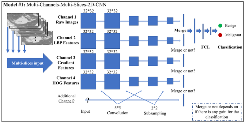
The major architecture of MCMS-2D CNN model.

Table 2:

Architecture of a standard two-channel MCMS-2D CNN model for Polyp dataset with parameters

2D-CNN	Channel 1	Channel 2
structure1	2D Convolutional Layer (5*5, 64)	2D Convolutional Layer (5*5, 64)
structure2	Activation “Relu”	Activation “Relu”
structure3	BatchNormalization	BatchNormalization
structure4	MaxPooling2D (2*2, strides=l)	MaxPooling2D (2*2, strides=l)
structure5	2D Convolutional Layer (5*5, 128)	2D Convolutional Layer (5*5, 128)
structure6	Activation “Relu”	Activation “Relu”
structure7	BatchNormalization	BatchNormalization
structure8	MaxPooling2D (2*2)	MaxPooling2D (2*2)
structure9	2D Convolutional Layer (5*5, 128)	2D Convolutional Layer (5*5, 128)
structure10	Activation “Relu”	Activation “Relu”
structure11	MaxPooling2D (2*2)	MaxPooling2D (2*2)
structure12	Dropout (0.5)	Dropout (0.5)
structure13	Flatten()	Flatten()
structure14	Merge(channel 1 &channel 2)
structure15	Dense
structure16	Dense
structure17	Dense, activation=softmax

2.2.2. Voxel-Level-ID CNN Model

In Section 2.2.1, we proposed the MCMS-2D CNN model with multi-channel and multislices inputs. Multi-channel can provide more feature maps and multi-slices can expand training samples significantly. However, the training samples from one subject/case is still small, resulting in only approximately dozens of slices with several channels. This is still far away from the expectation of training CNN models. So, we would like to pay more attention on how to significantly expand the training samples in this V-1D CNN model. The basic concept of V-1D CNN model is to generate training samples at the voxel-level. Instead of working on the whole slice each time for the classification, we would like to dedicate deep into the voxel level, study and abstract meaningful features for each voxel with a relatively small region of interested (ROI). In this way, the training samples can be extremely expanded. As an initial attempt, we would like to collect the intensity attributes surrounding each voxel and stretch those attributes as a 1D vector for the training dataset. An example is shown in the Figure 3B. In the V-1D CNN model, we will predict a label on the voxel level, either malignant or benign, by differentiating the pattern of their intensity attribute vectors.

Figure 3.

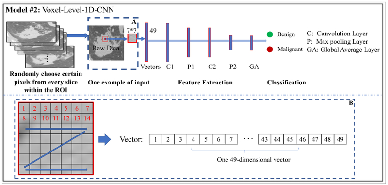
The major architecture of V-1D CNN model. Box A shows an example of extracting ROI from the voxel. Box B shows the details about how we stretch those attributes of ROI as a 1D vector for the training.

For this model, certain number of voxels are randomly chosen from each whole polyp/nodule volume to represent the characteristic of the whole volume of polyp/nodule. Their labels are given based on the label of whole polyp/nodule from the pathological report. In details, the total number of voxels we are prepared to select are prorated to each slice based on the size of polyp/nodule area for each slice, then the attributes of selected voxels are reshaped into vectors as the input, and then feed those vectors into the V-1D CNN model for the classification. The ROI is set to 7 * 7 as shown in Figure 3. Several 1D convolutional layers are added to the model, two convolutional layers are used for illustration, the size of the filter is set to 21 and 11, the number of the filter is set to 32 and 64, respectively. Global average layer is used to generate fully connected layer with output labels. ReLU is used as the activation function. Please refer to Table 3 for more details about the architecture of the V-1D CNN model.

Table 3:

Architecture of a standard V-1D CNN model for Lung nodule dataset with parameters

1D-CNN
structure1	1D Convolutional Layer (21,32)
structure2	BatchNormalization
structure3	Activation “Relu”
structure4	Maxpooling1D (2)
structure5	1D Convolutional Layer (11,64)
structure6	BatchNormalization
structure7	Activation “Relu”
structure8	Maxpooling1D (2)
structure9	GlobalAveragePooling1D
structure10	Dense, activation=softmax

2.2.3. Voting Algorithm

The above-mentioned CNN models are working on either slice level or voxel level, thus, voting algorithm will be utilized to gather the class of the polyp/nodule for each slice/voxel and then predict a final label for every testing polyp/nodule volume. Specifically, for the MCMS-2D CNN model, we will validate every slice of each testing polyp/nodule and determine whether malignant slices are significant. If significant, the polyp/nodule will be labeled as “1”, otherwise, labeled as “0”. For the V-1D CNN model, we will count the malignant voxels and benign voxels (voxels within the boundaries drawn by experts) and determine whether malignant voxels are significant. If malignant voxels are significant, the polyp/nodule will be labeled as “1”, otherwise, labeled as “0”. The general steps are summarized into the pseudocodes as follows:

Voting algorithm

function vote (x):

Input: x represents prediction labels of each slice/voxel of testing polyp/nodule

Output: Final label of the testing polyp/nodule

M(x) = the number of slices/voxels that x belongs to malignant (label of “1”);

B(x) = the number of slices/voxels that x belongs to benign (label of “0”);

Significant(x) = M(x)/(M(x)+B(x));

Whether Significant(x) is significant (e.g. we use 0.5 as a threshold to judge significant)

If yes,

then the testing polyp/nodule is labeled as “1”

If no,

then the testing polyp/nodule is labeled as “0”

Return the final label

After the application of the voting algorithm, the information from each slice/voxel can be gathered and summarized. Based on the voting strategies, we will have the final predictive label for each testing polyp/nodule.

2.3. Validation Strategy

Cross-validation is a validation technique for assessing how the results of a statistical analysis will generalize to an independent dataset. It is mainly used in settings where the goal is prediction, and one wants to estimate how accurately a predictive model will perform in practice. To evaluate the classification performance of the proposed CNN models, the cross-validation algorithm is utilized. Due to the small sample sizes, two most extreme cross-validation approaches are considered in this study: two-fold and leave-one-out cross-validations.

For the two-fold cross-validation, the whole sample is randomly divided into two equal parts. One part is used for training and the other is used for validation. Two-fold validation is an extreme case that the training set is the smallest compared to other fold validation (e.g. 10-fold or 5-fold validation). Therefore, the two-fold validation may have the worst performance of classification.

For the leave-one-out cross-validation, one polyp/nodule will be randomly selected at each time. All the polyps/nodules are used as the training set, and the left one is used for validation, repeat this procedure until all the polyps/nodules have been chosen as the left one and been used as the validation from the trained CNN models. The leave-one-out cross-validation is another extreme and it has the largest training set. Therefore, it may have the best classification performance. However, the shortage of the leave-one-out cross-validation is that sometimes overfitting may happen, and bias may be encountered in unbalanced datasets.

In summary, for the two small and unbalanced datasets, both two-fold and leave-one-out cross-validations were used to evaluate the classification performance for the proposed models. Multiple runs are adopted for both the two-fold cross-validation and the leave-one-out cross-validation, e.g. twenty runs for two-fold strategy and ten runs for leave-one-out strategy for proposed models, then the classification performances are averaged as the final performance. Due to the page limit, the results of two-fold cross validation under the toughest condition will be presented in this paper. The leave-one-out cross-validation is summarized in the Appendix as reference.

2.4. Statistical Analysis

To thoroughly understand the classification performance of the proposed models, the following commonly used validation measurements are used:

True positive (TP): malignant correctly identified as malignant.

False positive (FP): benign incorrectly identified as malignant.

True negative (TN): benign correctly identified as benign.

False negative (FN): malignant incorrectly identified as benign.

Accuracy (ACC): The correct prediction from the whole dataset.

$$ACC=\frac{TP+TN}{wholevalidationdataset}$$ (1)

True positive rate (TPR):

$$TPR=TP/\left(TP+FN\right)$$ (2)

False positive rate (FPR):

$$FPR=FP/\left(FP+TN\right)$$ (3)

Area under the curve (AUC): It is used in classification analysis in order to determine which of the used models predicts the classes best. An example of its application is receiver operating characteristic (ROC) curves. In ROC, the FPR is defined as x-axis and TPR is defined as y-axis.

Sensitivity (SE): the ability of the test to correctly identify those patients with the disease.

$$Sensitivity=\frac{TP}{TP+FP}$$ (4)

Specificity (SP): the specificity of a clinical test refers to the ability of the test to correctly identify those patients without the disease.

$$Specificity=\frac{TN}{TN+FN}$$ (5)

Based on above-mentioned validation measurements, we can have a better knowledge about the model we trained. In addition, AUC, ACC, SE and SP are used to evaluate the classification performance from different viewpoints. Also, we can use these measurements to compare the classification performance between different models. The advantages and disadvantages of proposed models can be well represented from these measurements.

3. Results

The proposed CNN models are implemented using Keras (the Python Deep Learning library) and Quadra P4000 is used as the GPU. Four different statistical measurements (i.e. AUC, ACC, SE and SP) are used for testing the validation performance. Two-fold cross validation strategy are used to show the classification performance in the results part.

3.1. Malignant-Benign Classification Performance on the Polyp Dataset

The MCMS-2D CNN model is applied on the polyp dataset. For each run, 31 polyps (16 malignant and 15 benign polyps) are randomly chosen as the training dataset, 32 remaining polyps (16 malignant and 16 benign polyps) are then automatically recognized as the validation dataset. Two channels are finally determined as raw images and LBP feature maps. In each channel, the size of each slice is set to 48*48, the total number of convolutional layers are three for each channel separately. The filter size is 5*5 and the number of filters for each layer is 64, 128 and 128, respectively. Twenty slices are used to represent one polyp volume. Please refer to Table 2 for more details about the architecture of the proposed CNN model.

3.1.1. Two-Fold Cross-Validation via MCMS-2D CNN Model

The average result of two-fold cross-validation are shown in Table 4. Both AUC (Mean±SD): 0.86±0.06 and ACC (Mean±SD): 0.83±0.06 are relatively consistent across the different runs. The results indicate that the MCMS-2D CNN model has reasonably good classification performance. In addition, the SE and SP are quite good, which have very important clinical impact. For the diagnosis on the pathologically proven datasets, SE represents the probability to correctly recognize the malignant polyp and it is clinically important because we should not ignore any malignant lesion. Then, to reveal the effectiveness of our proposed model, comparison experiments are adopted.

Table 4.

Classification performance of the MCMS-2D CNN model on the polyp dataset (Mean±SD).

Model	AUC	ACC	Sensitivity	Specificity
MCMS-2D CNN Model	0.86±0.06	0.83±0.06	0.85±0.07	0.79±0.11

3.1.2. Comparison between the Proposed Model and state-of-the-art Models

To better understand the classification performance of the MCMS-2D CNN model on the polyp dataset, we compared it to a traditional machine learning algorithm, i.e. the optimized Haralick texture model (Song et al., 2014; Hu et al., 2016), and several well-known CNN models, i.e. VGG-16 (Simonyan and Zisserman, 2014), VGG-19 (Simonyan and Zisserman, 2014) and AlexNet (Krizhevsky et al., 2012), the parameters from those models are carefully designed and optimized. The well published optimized Haralick texture model uses the Random Forest (RF) strategy to choose the representative features to do the classification, please refer to (Song et al., 2014; Hu et al., 2016) for more technique details. The classification results of all the comparison models are shown in the Appendix Table C1, the comparisons among those models are provided in the Figure 4. Compared our proposed CNN model with optimized Haralick texture model, the AUCs of two models are similar. However, the MCMS-2D CNN model has higher ACC, SE and SP than the optimized Haralick texture model. In addition, the standard deviations of the MCMS-2D CNN model is a little bit smaller than the optimized Haralick texture model, which means that the MCMS-2D CNN model has more consistent classification performance in different runs. Compared our proposed CNN model with other well-known CNN models, we can clearly identify that our proposed CNN model outperforms those well-known CNN models on this polyp dataset. Among three well-known CNN models, VGG-16 has better classification performance, AlexNet is the second and VGG-19 gets the worst performance.

Figure 4.

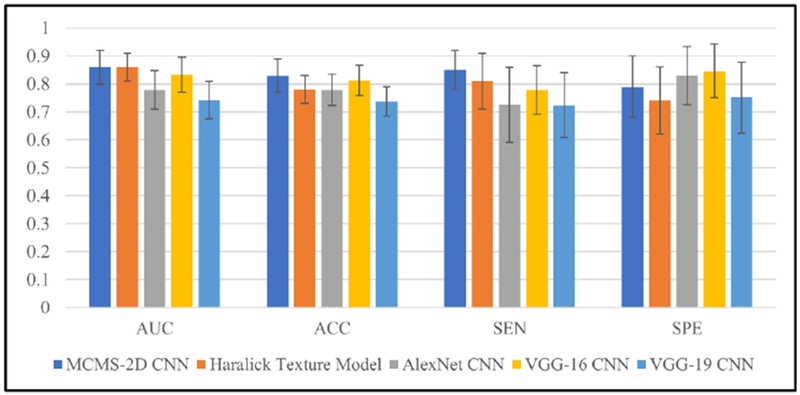
Classification performance from different models on the polyp dataset. For each validation measurement, results of all 5 models are shown by sequence with different color, means and standard deviations are shown in each bar.

We already know well that CNN architecture like VGG-16, VGG-19 and AlexNet work great for the big data classification, however for the small dataset, the classification performance dropped when the layers become deeper (e.g. VGG-16 is about 0.83 AUC, but VGG-19 is only 0.74 AUC). The possible reason is that when the layers go deeper, the advantage is that more abstract information can be extracted, but the disadvantage is also obvious, as more weights need to be trained which requires a larger training dataset. Thus, we believe that for the small medical image dataset, like the proposed pathologically proven dataset in this paper, instead of using those deep CNN architecture with many convolutional layers, some simple CNN architecture (like the MCMS-2D model we proposed) can also solve the classification problem quite well.

3.2. Malignant-Benign Classification Performance on the Lung Nodule Dataset

The lung nodule dataset is much more difficult to be classified than the polyp dataset, because it is not only a small dataset (only 67 lung nodules), but also badly unbalanced (18 benign and 49 malignant nodules). As we know, unbalanced dataset will significantly affect the training procedure, especially for the small dataset. Too small number of the training set from one category will be a big concern for the binary classification problem.

3.2.1. Two-Fold Cross-Validation via MCMS-2D CNN Model

To adopt the two-fold cross-validation for the proposed MCMS-2D CNN model on the lung nodule dataset, 34 nodules (24 malignant and 10 benign nodules) are randomly chosen as the training set in each run, and the remaining 33 nodules (25 malignant and 8 benign modules) are then automatically recognized as the testing set. Two channels are finally determined as raw images and LBP feature images. In each channel, the size of each slice is set to 32*32, and the total number of convolutional layers is two for each channel separately. The filter size is 5*5 and the number of filters for each layer is 64 and 128, respectively. Ten slices will be used to represent one lung nodule.

The classification performance of the MCMS-2D CNN model is shown in Table 5. The classification performance is obviously dropped compared with the performance of the polyp dataset, and it is believed to be reasonable because this dataset is extremely unbalanced. In the training set, there are only 10 benign nodules and 10 slices for each nodule, which means that there are only 100 slices for the benign category. Since the CNN models require large datasets, there is a major concern that insufficient learning may occur in the training process.

Table 5.

Classification performance of MCMS-2D CNN model on lung nodule dataset (Mean±SD).

Model	AUC	ACC	Sensitivity	Specificity
MCMS-2D CNN Model	0.66±0.09	0.77±0.03	0.76±0.09	0.46±0.16

3.2.2. Two-Fold Cross-Validation via V-1D CNN Model

To overcome the challenge of unbalanced, the V-1D CNN model was adopted to analyze the lung nodule dataset. Similar to Section 3.2.1, 34 nodules (24 malignant and 10 benign nodules) are randomly chosen as the training set in each run, and the remaining 33 nodules (25 malignant and 8 benign modules) are then automatically recognized as the testing set. The ROI is set to 7 * 7, two 1D convolutional layers are added to the model, the size of the filter is set to 21 and 11, respectively. In total, 2000 voxels are picked up from each lung nodule volume. The proposed model can extremely expand the training samples, as we mentioned in the Section 2.2.2, and this model should be less affected by insufficient learning problem. Please refer to Table 3 for more details about the architecture of the proposed CNN model. The classification performance of the V-1D CNN model is shown in Table 6.

Table 6.

Classification performance of V-1D CNN model on the lung nodule dataset (Mean±SD).

Model	AUC	ACC	Sensitivity	Specificity
V-1D CNN Model	0.71±0.08	0.78±0.03	0.8±0.11	0.53±0.15

The results show that the V-1D CNN model achieves better performance than the MCMS-2D CNN model, especially for AUC, SE and SP (ACC has less meaning in unbalanced dataset), with approximate 5% improvement in each measure. Although the number of malignant training samples is still much larger than benign training samples, the V-1D CNN model can successfully study the differences between benign and malignant lesions based on the voxel level training samples we generated. The bias caused by the large malignant training set is less in the V-1D CNN model than the MCMS-2D CNN model. The main reason of the V-1D CNN model having overall better performance could be that the V-1D CNN model can offer sufficient training samples even the training dataset is badly unbalanced. This will help to avoid the insufficient learning problem from the category with less cases. As a result, V-1D CNN model is more suitable for the small and unbalanced dataset.

3.2.3. Comparison among Proposed Models and state-of-the-art Models

Similar to the analysis of the polyp dataset, we also tested the lung nodule dataset using the optimized Haralick texture model and well-known CNN models to compare the classification performance with two proposed models, the classification performance results are shown in the Appendix Table D1. The comparison performances among all the models are shown in Figure 5. Between our proposed two CNN models, the MCMS-2D CNN model has inferior classification performance than the V-1D CNN model in all validation measures, which may possibly due to insufficient learning. In addition, among our proposed two models and the optimized Haralick texture model, the optimized Haralick texture model has the lowest values of AUC, ACC and SP but not SE. This finding indicates that CNN models have the potential ability to achieve better classification performance even when the dataset is quite small and unbalanced. Furthermore, we compared the well-known CNN models with our proposed CNN models, the results are very interesting. When we use deep CNN architecture to study this dataset, we found that the specificity measurement is very small (around 0-0.15), but the sensitivity is almost consistent to 1, this phenomenon clearly indicates that it is tough for deep CNN to study this dataset, therefore, most cases are identified as malignancy. The possible reason is that most cases from this dataset are malignancy, it is hard to learn abstract features from benign ones within such a small number of cases, thus no representative and distinguishable features are well trained and learned. This is additional evidence that we should design unique models to deal with small datasets.

Figure 5.

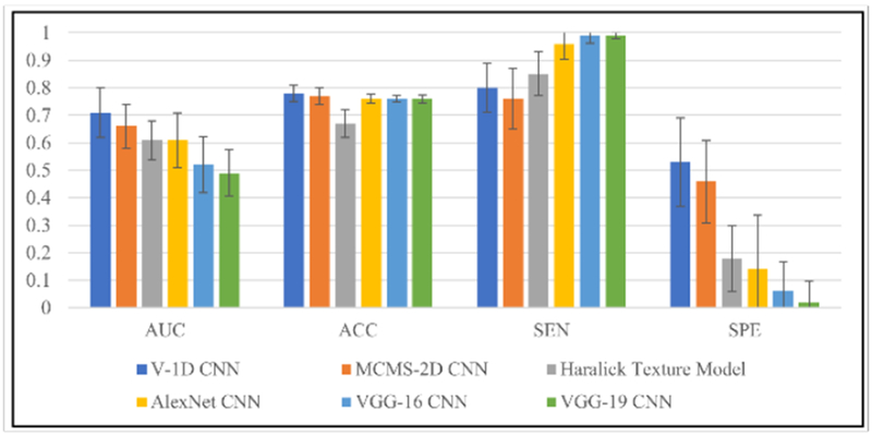
Classification performance from different models on lung nodule dataset. For each validation measurement, results of all the models are shown by sequence with different color. Means and standard deviations are shown in each bar.

By studying large number of local regions from malignant and benign nodules, the V-1D CNN model can achieve around 0.71 AUC and it demonstrates that V-1D CNN model indeed works well for the small and unbalanced datasets. Due to the shortage of the training samples, the MCMS-2D model works a little bit worse, but still achieve reasonable classification performance. We also find that by feeding voxel-level local information into the V-1D CNN model, we can achieve quite good classification performance, that is to say, local information from malignances and benigns are also distinguishable. This is a very interesting finding, we always want to differentiate malignant from benign lesions via whole volume, however, too many overlap information in the whole volumes will bias the results when we identify malignant or benign lesion at whole volume level. Instead, V-1D CNN model gives another way of thinking, we can identify malignant from benign lesions firstly at voxel level and then predict the final label for the whole volume via voting algorithm.

4. Discussion and Conclusion

In this paper, we proposed two CNN models to identify the malignant from benign lesions and adopt the models to two small and unbalanced pathologically proven datasets. This work is at an early stage of the field which adopts deep learning approaches to focus on pathologically proven datasets. The MCMS-2D CNN model can achieve relatively good classification performance in small datasets, and the model is very consistent across different datasets. However, the V-1D CNN model works better for the small and unbalanced dataset. Its power of extremely expanding the training set provides lots of benefits for the classification on the unbalanced dataset. In general, the results demonstrated that the proposed models have their own advantages on studying small datasets. Reasonably good classification performance can be achieved on two datasets, e.g. 0.86 AUC for the polyp dataset and 0.71 AUC for the lung nodule dataset.

The first thing worth noticing again is always about the dataset. We would like to claim again that studying the pathologically proven datasets are necessary. In previous studies, most researches use datasets without the pathologically record, which brings a very serious concern about the ground truth labeling of those nodules/polyps. In order words, how to avoid the labeling noises is crucial. Litjens et al. (2017) showed an example about the widely used lung CT LIDC-IDRI dataset (Armato et al., 2011). In the LIDC-IDRI dataset, pulmonary nodules were annotated by four radiologists independently, those experts reviewed annotations from others, but no consensus was forced. The results showed that only 25% nodules are totally agreed to be a nodule, for the others, they could not reach clearly conclusions (Armato et al., 2011). Han et al. (2015) showed another example that when the label definition of the nodule is different in the LIDC-IDRI dataset, the classification performances are largely different (one is about 0.91 AUC, another one is about 0.78 AUC). Thus, when using those datasets, we should have careful consideration of how to deal with noise and uncertainty. Even though quite good classification performances have been achieved from many studies using datasets without the pathologically record (e.g. studies using the LIDC-IDRI dataset), the real performance of differentiating malignant from benign lesions is still not fully known yet. One simple and straightforward solution is, to use the pathologically proven datasets.

Since the pathologically proven datasets are always small, we need to design a proper CNN model to fit for the small data. In this study, we pointed out that instead of studying the raw CT images only, we would like to study the feature images of the raw CT images too. The strategy is using multi-channel CNN to feed the raw images and their feature images into the model via different channels and study them simultaneously. The main idea is if we don’t have large dataset to thoroughly train the CNN model, can we directly send meaningful feature images to the CNN model and train the CNN model to achieve better classification performance? In Section 2.2.1, we designed our model with multiple channels, and we examined three commonly used feature images to verify our ideas. The conclusion is that additional feature images indeed improved the classification performance of the trained CNN model. In details, when only raw images were used, the classification of MCMS-2D CNN on the polyp dataset is about 0.78 AUC. When the LBP feature images were added as the second channel, the MCMS-2D CNN model can achieve around 0.86 AUC, which is a huge improvement. However, when the third channel was added with either gradient images or HOG feature images, there were no further gains, and this phenomenon is consistent with the lung nodule dataset. This indicates that, adding proper feature images could help to train better classification performance when the dataset is small. Furthermore, the results show that, for the polyp and lung nodule diagnosis, LBP features are more important than gradient images and HOG feature images as it will bring more effective features for the model to differentiate malignant from benign lesions. To show the effectiveness of the MCMS-2D CNN model we proposed, the average AUC of different experiment designs are listed in Table 7.

Table 7.

Average AUC of different experiment designs on the polyp dataset.

	Max-Slice-Raw	Multi-Slices-Raw	MCMS-Raw-LBP-10Slices	MCMS-Raw-LBP-20Slices
AUC	0.76	0.78	0.82	0.86

As shown in Table 7, AUC progressed as more slices and LBP added to the MCMS-2D CNN model. Only 0.76 AUC was achieved when one slice with max region of polyp tissues from each polyp was used to train the CNN model. There was 2% improvement in AUC by using multi slices from each polyp, 4% additional improvement by using multiple channels and finally 4% more improvement by using the proper number of slices for each polyp volume.

However, pathologically proven datasets are not only small but also very unbalanced at times, e.g. the lung nodule dataset in this study. It will become tougher for the MCMS-2D CNN model to overcome the unbalanced problem even with multi-channel and multi-slice inputs. The classification results of differentiating the lung nodule dataset using the MCMS-2D CNN model demonstrated that the number of the inputs were still quite small for the unbalanced dataset. Like studies in Liu et al. (2018), Zhang et al. (2018) and Oliveira and Viana (2018), the voxel level 1D CNN model has its superiority and can achieve reasonably good classification performance. These studies inspired us to propose a V-1D CNN model to extremely expand the training samples at the voxel level and overcome the small and unbalanced issues. From the results shown in the Section 3.2, the results indicate that V-1D CNN model has big advantage to overcome small and unbalanced issues. Its superpower of expanding the training samples can help the CNN model to study from huge number of inputs, which will provide more benefits than the noises the method produced. Of course, the V-1D CNN model has its own concerns and shortages, e.g. 1D signals contains less information when compared with 2D slices or 3D cubes. But, on the other hand, the training samples are expanding significantly, which will help us to train better CNN models with better classification performance. In the V-1D CNN model, two important parameters need more attention. One key factor is to confirm the level of the down-sampling to represent whole polyp/lung nodule. In this study, 1000 and 2000 voxels per polyp/nodule volume were explored and 2000 voxels achieved the best performance. The other one is the size of the ROI (local region) for each voxel, 5*5 square and 7*7 square were explored, and 7*7 square performed better. These two parameters will affect the classification performance a lot and furthermore studies are needed to better understand the relationship between these two parameters and the classification performances and may reveal key information to differentiate malignant from benign lesions.

In addition to the two-fold cross-validation approach, the leave-one-out cross-validation were also utilized, and the results are presented in the Appendix. For the polyp dataset, the MCMS-2D CNN model achieved similar classification performances between the two-fold and leave-one-out cross-validation approaches. For the lung nodule dataset, the two-fold cross-validation approach outperformed the leave-one-out cross-validation approach. This interesting phenomenon demonstrated that bias will be produced into leave-one-out cross-validation when this dataset is not only small but also unbalanced and this bias will greatly affect the MCMS-2D CNN model. However, the classification performance of V-1D CNN model is still quite good and consistent between two-fold and leave-one-out cross-validation performances, indicating that the V-1D CNN model can not only overcome the bias from the unbalanced dataset, but also achieve good classification performance via studying the local information.

In summary, the MCMS-2D CNN model can offer good classification performance if the dataset has reasonably amount of training samples. Another important finding about the MCMS-2D CNN model is that if some typical feature images (e.g. the LBP pattern of the raw images) are manually added as extra inputs, the classification performance can be improved, especially for the small dataset. Furthermore, if the dataset is too small and unbalanced, V-1D CNN model can offer better performance via extremely expanding the training samples. Even though the V-1D CNN model has its own limitations, we find the importance of the voxel-level concept, which can overcome extremely small sample size and unbalanced issues and achieve meaningful results.

The limitations for the proposed CNN models are also provided here for the discussion. First, setting and tuning the parameters from the CNN models are still the key problems but very challenging. For example, for the MCMS-2D CNN model, the number of the slices we want to use largely dependents on the dataset itself, it could be varied a lot for different datasets, which is quite time consuming to search for the proper values; similar to the V-1D CNN model, when we use voxel level concept, the number of the voxels we would like to pick up from the whole volume is quite important and those numbers will significantly impact the classification results, so the down-sampling rate is important but need to be tested to achieve the good result. Second, the proposed CNN models still didn’t fully study all the information from the dataset. In the MCMS-2D CNN model, we fix the number of slices we would like to use for each volume, thus some slices may not be used at all; similar to V-1D CNN model, for the voxels we picked up, the representative features will be generated from 2D matrix into 1D vectors, as we shown in the Figure 3B, some topology information will be missed during this process. Those are the key factors to optimize our proposed models and additional improvement can be expected.

For the future work, on one hand, we will continue collecting polyps/nodules with pathology reports to enrich our pathologically proven datasets. On the other hand, we would like to further optimize the proposed CNN models. For the MCMS-2D CNN model, we would like to firstly study how to better tune the parameters for the model, then we will investigate on collecting and feeding more texture features to the CNN models to pursuit better classification performance. For the V-1D CNN model, we also would like to first study how to better tune the parameters for the model, then apply this voxel-level concept onto voxel-level two-dimensional (V-2D) CNN or voxel-level three-dimensional (V-3D) CNN models to both expanding the training samples and include more information for each voxel. We believe that more information for each voxel will let us study the data better and bring us better classification performance. In addition, we would like to further investigate whether local information could provide additional help to diagnosis malignant/benign lesions and we will optimize our models once we enlarge our pathologically proven datasets.

Figure 1.

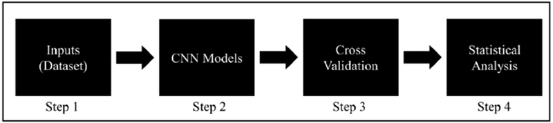
The flowchart of our proposed pipeline.

Highlights.

• Proposed two CNN models to classify small cancer image dataset (Malignance/Benign).

• Combine raw images and LBP features can improve the classification on small data.

• Proposed V-1D model can better study the small and unbalanced dataset.

• Local information from lung nodule significantly improves the M/B classification.

Appendix

A. Leave-One-Out Cross-Validation Performance via the MCMS-2D CNN Model on the Polyp Dataset

Average results of the leave-one-out cross-validation approach for the polyp dataset are shown in the Table A.1. The MCMS-2D CNN model achieved 0.87 AUC, with a standard deviation of 0.02. Both SE and SP are relatively high, and ACC is 0.84. These results demonstrate the robustness of the proposed MCMS-2D CNN Model.

Table A.1.

Classification performance of the MCMS-2D CNN model on the polyp dataset using the leave-one-out cross validation (Mean±SD).

Model	AUC	ACC	Sensitivity	Specificity
MCMS-2D CNN Model	0.87±0.02	0.84±0.02	0.89±0.02	0.75±0.04

B. Leave-One-Out Cross-Validation Performance via the proposed CNN models on the Lung Nodule dataset

Average results of the leave-one-out cross-validation approach for the lung nodule dataset are shown in Table B.1. The performance of MCMS-2D CNN model is poor with an AUC of 0.55 and a SP of 0.22. On the contrary, the V-1D CNN model has better performance, AUC is approximate 0.70 with a standard deviation of 0.04. SE is comparable to the performance of the MCMS-2D CNN mode, while SP is 25% better than the MCMS-2D CNN model.

Table B.1.

Classification performance of proposed CNN models on lung nodule dataset (Mean±SD).

Model	AUC	ACC	Sensitivity	Specificity
MCMS-2D CNN Model	0.55±0.07	0.74±0.01	0.83±0.12	0.22±0.17
V-1D CNN Model	0.70±0.03	0.76±0.03	0.80±0.05	0.47±0.05

The results of Appendix A and Appendix B are averaged from 10 separate runs.

C. Two-Fold Cross-Validation Performance via the comparison models on the Polyp Dataset

Table C.1.

Classification performance of several well-known CNN architectures on polyp dataset.

Model	AUC	ACC	Sensitivity	Specificity
Alex-net CNN	0.78±0.07	0.78±0.06	0.73±0.13	0.83±0.10
Vgg-16 CNN	0.83±0.06	0.81±0.06	0.78±0.09	0.85±0.10
Vgg-19 CNN	0.74±0.07	0.74±0.05	0.72±0.12	0.75±0.13
Haralick Feature RF	0.86±0.05	0.78±0.05	0.81±0.10	0.74±0.12

D. Two-Fold Cross-Validation Performance via the comparison models on the Lung Nodule Dataset

Table D.1.

Classification performance of several well-known CNN architectures on lung nodule dataset.

Model	AUC	ACC	Sensitivity	Specificity
Alex-net CNN	0.61±0.10	0.76±0.02	0.96±0.06	0.14±0.20
Vgg-16 CNN	0.52±0.10	0.76±0.01	0.99±0.03	0.06±0.11
Vgg-19 CNN	0.49±0.08	0.76±0.01	0.99±0.01	0.02±0.08
Haralick Feature RF	0.61±0.07	0.67±0.05	0.85±0.08	0.18±0.12

References

- Armato SG, McLennan G, Bidaut L, McNitt-Gray MF, Meyer CR, Reeves AP, et al. , 2011. The lung image database consortium (LIDC) and image database resource initiative (IDRI): a completed reference database of lung nodules on CT scans. Medical physics, 38(2), 915–931. [DOI] [PMC free article] [PubMed] [Google Scholar]
- Bipat S, Glas AS, Slors FJ, Zwinderman AH, Bossuyt PM, Stoker J, 2004. Rectal cancer: local staging and assessment of lymph node involvement with endoluminal US, CT, and MR imaging—a meta-analysis. Radiology, 232(3), 773–783. [DOI] [PubMed] [Google Scholar]
- Chakraborty A, Staib LH, Duncan JS, 1996. Deformable boundary finding in medical images by integrating gradient and region information. IEEE Transactions on Medical Imaging, 15(6), 859–870. [DOI] [PubMed] [Google Scholar]
- Chen YK, Ding HJ, Su CT, Shen YY, Chen LK, Liao AC, Hung TZ, Hu FL, KAO CH, 2004. Application of PET and PET/CT imaging for cancer screening. Anticancer research, 24(6), 4103–4108. [PubMed] [Google Scholar]
- Ciompi F, de Hoop B, van Riel SJ, Chung K, Scholten ET, Oudkerk M, de Jong PA, Prokop M, van Ginneken B, 2015. Automatic classification of pulmonary peri-fissural nodules in computed tomography using an ensemble of 2D views and a convolutional neural network out-of-the-box. Medical image analysis, 26(1), 195–202. [DOI] [PubMed] [Google Scholar]
- Dalal N, Triggs B, 2005. Histograms of oriented gradients for human detection. In international Conference on computer vision & Pattern Recognition, Vol. 1, pp. 886–893. [Google Scholar]
- Dellana R, Roy K, 2016. Data augmentation in CNN-based periocular authentication. In 2016 6th International Conference on Information Communication and Management, pp. 141–145. [Google Scholar]
- Deng J, Dong W, Socher R, Li LJ, Li K, Li FF, 2009. Imagenet: A large-scale hierarchical image database, pp. 248–255. [Google Scholar]
- Deng L, Yu D, 2014. Deep learning: methods and applications. Foundations and Trends® in Signal Processing, 7(3-4), 197–387. [Google Scholar]
- Doi K, 2007. Computer-aided diagnosis in medical imaging: historical review, current status and future potential. Computerized medical imaging and graphics, 31(4-5), 198–211. [DOI] [PMC free article] [PubMed] [Google Scholar]
- Forstner R, Hricak H, Occhipinti KA, Powell CB, Frankel SD, Stem JL, 1995. Ovarian cancer: staging with CT and MR imaging. Radiology, 197(3), 619–626. [DOI] [PubMed] [Google Scholar]
- Frangioni JV, 2008. New technologies for human cancer imaging. Journal of clinical oncology, 26(24), 4012. [DOI] [PMC free article] [PubMed] [Google Scholar]
- Gurney JW, 1996. Missed lung cancer at CT: imaging findings in nine patients. Radiology, 199(1), 117–122. [DOI] [PubMed] [Google Scholar]
- Han F, Wang H, Zhang G, Han H, Song B, Li L, Moore W, Lu H, Zhao H, Liang Z, 2015. Texture feature analysis for computer-aided diagnosis on pulmonary nodules. Journal of digital imaging, 28(1), 99–115. [DOI] [PMC free article] [PubMed] [Google Scholar]
- Hua KL, Hsu CH, Hidayati SC, Cheng WH, Chen YJ, 2015. Computer-aided classification of lung nodules on computed tomography images via deep learning technique. Onco Targets and therapy, 8. [DOI] [PMC free article] [PubMed] [Google Scholar]
- Hu Y, Liang Z, Song B, Han H, Pickhardt PJ, Zhu W, Duan D, Zhang H, Barish MA, Lascarides CE, 2016. Texture feature extraction and analysis for polyp differentiation via computed tomography colonography. IEEE transactions on medical imaging, 35(6), 1522–1531. [DOI] [PMC free article] [PubMed] [Google Scholar]
- International Early Lung Cancer Action Program Investigators, 2006. Survival of patients with stage I lung cancer detected on CT screening. New England Journal of Medicine, 355(17), 1763–1771. [DOI] [PubMed] [Google Scholar]
- Jayasurya K, Fung G, Yu S, Dehing-Oberije C, De Ruysscher D, Hope A, De Neve W, Lievens Y, Dekker ALAJ, 2010. Comparison of Bayesian network and support vector machine models for two-year survival prediction in lung cancer patients treated with radiotherapy. Medical physics, 37(4), 1401–1407. [DOI] [PubMed] [Google Scholar]
- Keuper M, Tang S, Zhongjie Y, Andres B, Brox T, Schiele B, 2016. A multi-cut formulation for joint segmentation and tracking of multiple objects arXiv preprint arXiv: 1607.06317. [Google Scholar]
- Krizhevsky A, Sutskever I, Hinton GE, 2012. Imagenet classification with deep convolutional neural networks In Advances in neural information processing systems (pp. 1097–1105). [Google Scholar]
- LeCun Y, Bengio Y, Hinton G, 2015. Deep learning. nature, 521(7553), 436. [DOI] [PubMed] [Google Scholar]
- Li Q, Cai W, Wang X, Zhou Y, Feng DD, Chen M, 2014. Medical image classification with convolutional neural network. In 2014 13th International Conference on Control Automation Robotics & Vision, pp. 844–848. [Google Scholar]
- Litjens G, Kooi T, Bejnordi BE, Setio AAA, Ciompi F, Ghafoorian M, van der Laak JAWM, van Ginneken B, Sanchez CI, 2017. A survey on deep learning in medical image analysis. Medical image analysis, 42, 60–88. [DOI] [PubMed] [Google Scholar]
- Liu H, Zhang S, Jiang X, Zhang T, Huang H, Ge F, Zhao L, Li X, Hu X, Han J, Guo L, Liu T, 2018. The Cerebral Cortex is Bisectionally Segregated into Two Fundamentally Different Functional Units of Gyri and Sulci. Cerebral Cortex. [DOI] [PMC free article] [PubMed] [Google Scholar]
- Lo SC, Lou SL, Lin JS, Freedman MT, Chien MV, Mun SK, 1995. Artificial convolution neural network techniques and applications for lung nodule detection. IEEE Transactions on Medical Imaging, 14(4), 711–718. [DOI] [PubMed] [Google Scholar]
- Milletari F, Navab N, & Ahmadi SA, 2016. V-net: Fully convolutional neural networks for volumetric medical image segmentation. In 2016 Fourth International Conference on 3D Vision, pp. 565–571. [Google Scholar]
- Mnih V, Kavukcuoglu K, Silver D, Graves A, Antonoglou I, Wierstra D, Riedmiller M, 2013. Playing atari with deep reinforcement learning arXiv preprint arXiv:1312.5602. [Google Scholar]
- Mudigonda NR, Rangayyan R, Desautels JL, 2000. Gradient and texture analysis for the classification of mammographic masses. IEEE transactions on medical imaging, 19(10), 1032–1043. [DOI] [PubMed] [Google Scholar]
- Nanni L, Lumini A, Brahnam S, 2010. Local binary patterns variants as texture descriptors for medical image analysis. Artificial intelligence in medicine, 49(2), 117–125. [DOI] [PubMed] [Google Scholar]
- Nanni L, Lumini A, Brahnam S, 2012. Survey on LBP based texture descriptors for image classification. Expert Systems with Applications, 39(3), 3634–3641. [Google Scholar]
- Ngiam J, Khosla A, Kim M, Nam J, Lee H, Ng AY, 2011. Multimodal deep learning. In Proceedings of the 28th international conference on machine learning, pp. 689–696. [Google Scholar]
- Ojala T, Pietikainen M, Harwood D, 1996. A comparative study of texture measures with classification based on featured distributions. Pattern recognition, 29(1), 51–59. [Google Scholar]
- Oliveira DAB., Viana MP., 2018. Using 1D Patch-Based Signatures for Efficient Cascaded Classification of Lung Nodules. In International Workshop on Patchbased Techniques in Medical Imaging, pp. 67–75. [Google Scholar]
- Popovtzer R, Agrawal A, Kotov NA, Popovtzer A, Balter J, Carey TE, Kopelman R, 2008. Targeted gold nanoparticles enable molecular CT imaging of cancer. Nano letters, 8(12), 4593–4596. [DOI] [PMC free article] [PubMed] [Google Scholar]
- Quan TM, Hildebrand DG, Jeong WK, 2016. Fusionnet: A deep fully residual convolutional neural network for image segmentation in connectomics arXiv preprint arXiv:1612.05360. [Google Scholar]
- Ribeiro E, Uhl A, Hafner M, 2016. Colonic polyp classification with convolutional neural networks. In 2016 IEEE 29th International Symposium on Computer-Based Medical Systems, pp. 253–258. [Google Scholar]
- Rouhi R, Jafari M, Kasaei S, Keshavarzian P, 2015. Benign and malignant breast tumors classification based on region growing and CNN segmentation. Expert Systems with Applications, 42(3), 990–1002. [Google Scholar]
- Sahiner B, Chan HP, Petrick N, Wei D, Helvie MA, Adler DD, Goodsitt MM, 1996. Classification of mass and normal breast tissue: a convolution neural network classifier with spatial domain and texture images. IEEE transactions on Medical Imaging, 15(5), 598–610. [DOI] [PubMed] [Google Scholar]
- Salamon J, Bello JP, 2017. Deep convolutional neural networks and data augmentation for environmental sound classification. IEEE Signal Processing Letters, 24(3), 279–283. [Google Scholar]
- Schmidhuber J, 2015. Deep learning in neural networks: An overview. Neural networks, 61, 85–117. [DOI] [PubMed] [Google Scholar]
- Shen W, Zhou M, Yang F, Yang C, Tian J, 2015. Multi-scale convolutional neural networks for lung nodule classification. In International Conference on Information Processing in Medical Imaging, pp. 588–599. [DOI] [PubMed] [Google Scholar]
- Shen W, Zhou M, Yang F, Yu D, Dong D, Yang C, Zang Y, Tian J, 2017. Multi-crop convolutional neural networks for lung nodule malignancy suspiciousness classification. Pattern Recognition, 61, 663–673. [Google Scholar]
- Shin HC, Roth HR, Gao M, Lu L, Xu Z, Nogues I, Yao J, Mollura D, Summers RM, 2016. Deep convolutional neural networks for computer-aided detection: CNN architectures, dataset characteristics and transfer learning. IEEE transactions on medical imaging, 35(5), 1285–1298. [DOI] [PMC free article] [PubMed] [Google Scholar]
- Simonyan K, Zisserman A, 2014. Very deep convolutional networks for large-scale image recognition arXiv preprint arXiv: 1409.1556. [Google Scholar]
- Song B, Zhang G, Lu EL, Wang EL, Zhu W, Pickhardt PJ, Liang Z, 2014. Volumetric texture features from higher-order images for diagnosis of colon lesions via CT colonography. International journal of computer assisted radiology and surgery, 9(6), 1021–1031. [DOI] [PMC free article] [PubMed] [Google Scholar]
- Song L, Liu X, Ma L, Zhou C, Zhao X, Zhao Y, 2012. Using HOG-LBP features and MMP learning to recognize imaging signs of lung lesions. In 2012 25th IEEE International Symposium on Computer-Based Medical Systems, pp. 1–4. [Google Scholar]
- Song Y, Cai W, Zhou Y, & Feng DD, 2013. Feature-based image patch approximation for lung tissue classification. IEEE transactions on medical imaging, 32(4), 797–808. [DOI] [PubMed] [Google Scholar]
- Sun T, Wang J, Li X, Lv P, Liu F, Luo Y, Gao Q, Zhu EL, Guo X, 2013. Comparative evaluation of support vector machines for computer aided diagnosis of lung cancer in CT based on a multi-dimensional data set. Computer methods and programs in biomedicine, 111(2), 519–524. [DOI] [PubMed] [Google Scholar]
- Sun W, Zheng B, Qian W, 2016. Computer aided lung cancer diagnosis with deep learning algorithms In Medical imaging 2016: computer-aided diagnosis, Vol. 9785, p. 97850Z. [Google Scholar]
- Tajbakhsh N, Shin JY, Gurudu SR, Hurst RT, Kendall CB, Gotway MB, Liang J, 2016. Convolutional neural networks for medical image analysis: Full training or fine tuning? IEEE transactions on medical imaging, 35(5), 1299–1312. [DOI] [PubMed] [Google Scholar]
- Unay D, Ekin A, Cetin M, Jasinschi R, Ercil A, 2007. Robustness of local binary patterns in brain MR image analysis. In 2007 29th Annual International Conference of the IEEE Engineering in Medicine and Biology Society, pp. 2098–2101. [DOI] [PubMed] [Google Scholar]
- Van Opbroek A, Ikram MA, Vemooij MW, De Bruijne M, 2015. Transfer learning improves supervised image segmentation across imaging protocols. IEEE transactions on medical imaging, 34(5), 1018–1030. [DOI] [PubMed] [Google Scholar]
- Wang CM, Mai XX, Lin GC, Kuo CT, 2008. Classification for breast MRI using support vector machine. In 2008 IEEE 8th International Conference on Computer and Information Technology Workshops, pp. 362–367. [Google Scholar]
- Wigington C, Stewart S, Davis B, Barrett B, Price B, Cohen S, 2017. Data augmentation for recognition of handwritten words and lines using a cnn-lstm network. In 2017 14th IAPR International Conference on Document Analysis and Recognition, Vol. 1, pp. 639–645. [Google Scholar]
- Wong SC, Gatt A, Stamatescu V, McDonnell MD, 2016. Understanding data augmentation for classification: when to warp? In 2016 international conference on digital image computing: techniques and applications, pp. 1–6. [Google Scholar]
- World Health Organization, 2018. Cancer, https://www.who.int/news-room/fact-sheets/detail/cancer.
- Yedroudj M, Chaumont M, Comby F, 2018. How to augment a small learning set for improving the performances of a CNN-based steganalyzer? Electronic Imaging, 2018(7), 1–7. [Google Scholar]
- Zhang R, Zheng Y, Mak TWC, Yu R, Wong SH, Lau JY, Poon CC, 2017. Automatic detection and classification of colorectal polyps by transferring low-level CNN features from nonmedical domain. IEEE journal of biomedical and health informatics, 21(1), 41–47. [DOI] [PubMed] [Google Scholar]
- Zhang S, Liu H, Huang H, Zhao Y, Jiang X, Bowers B, Guo L, Hu X, Sanchez M, Liu T, 2018. Deep Learning Models Unveiled Functional Difference between Cortical Gyri and Sulci. IEEE Transactions on Biomedical Engineering. [DOI] [PMC free article] [PubMed] [Google Scholar]
- Zięba M, Tomczak JM, Lubicz M, Świątck J, 2014. Boosted SVM for extracting rules from imbalanced data in application to prediction of the post-operative life expectancy in the lung cancer patients. Applied soft computing, 14, 99–108. [Google Scholar]