Functional Logistic Mixed-Effects Models for Learning Curves From Longitudinal Binary Data

Abstract

Purpose

We present functional logistic mixed-effects models (FLMEMs) for estimating population and individual-level learning curves in longitudinal experiments.

Method

Using functional analysis tools in a Bayesian hierarchical framework, the FLMEM captures nonlinear, smoothly varying learning curves, appropriately accommodating uncertainty in various aspects of the analysis while also borrowing information across different model layers. An R package implementing our method is available as part of the Supplemental Materials.

Results

Application to speech learning data from Reetzke, Xie, Llanos, and Chandrasekaran (2018) and a simulation study demonstrate the utility of FLMEM and its many advantages over linear and logistic mixed-effects models.

Conclusion

The FLMEM is highly flexible and efficient in improving upon the practical limitations of linear models and logistic linear mixed-effects models. We expect the FLMEM to be a useful addition to the speech, language, and hearing scientist's toolkit.

Supplemental Material

https://doi.org/10.23641/asha.7822568

Research in the speech, language, and hearing sciences often involves longitudinal data analysis (Jia, 2003; Reetzke et al., 2018). Whereas some investigations focus on the developmental trajectories of language learning across different groups (e.g., differences in learning one language vs. two languages in early childhood; Bialystok, Luk, Peets, & Yang, 2010; Pearson, Fernández, & Oller, 1993; Uccelli & Páez, 2007), others focus on the benefits of new intervention strategies for populations with various speech, language, and hearing impairments over time (e.g., speech-in-noise hearing strategies for older adults with hearing loss; Anderson, White-Schwoch, Choi, & Kraus, 2014; Anderson, White-Schwoch, Parbery-Clark, & Kraus, 2013; Burk & Humes, 2008). Trial-by-trial data generated by such experiments are usually treated as binary in nature (e.g., accuracy on a behavioral task), recording whether the participants were successful in their assigned task or not. The underlying “learning curve” may then be defined as the average longitudinal trajectory of the probability of success in the population of interest. In doing so, it is important to accommodate the individual heterogeneity of the participants. For example, in studies examining participant learning across time, one participant may take a longer time to learn a given task relative to others (Wong, Perrachione, & Parrish, 2007; Zatorre, 2013). The experimental designs and scientific questions of interest thus naturally give rise to mixed-effects models, where the primary interest is in estimating the population-level learning curve whereas secondary interests lie in inferring individual variability related to participant-level behavior.

Research employing mixed-effects models for inference in such data sets has focused primarily on linear mixed-effects models or their many variants, including analysis of variance models (Holt, Lee, Dowell, & Vogel, 2018; Ingvalson, Lansford, Fedorova, & Fernandez, 2017; Jia, 2003; Moyle, Ellis Weismer, Evans, & Lindstrom, 2007), often implemented using the lme4 package in R. Such models are, however, not very suitable for modeling quantities with restricted supports, for example, probabilities. In nonlongitudinal static settings, Jaeger (2008) promoted the use of generalized linear models instead, specifically the logistic mixed model. Such models regress logit-transformed probabilities, which are no longer supported only on [0, 1] but can technically take any value on the real line, on associated covariates using traditional linear mixed models. An alternative data transformation is the arcsine function, $\theta =arcsin\sqrt{p}$. However, as noted in Warton and Hui (2011), this transformation lacks both testing power and interpretability. Moreover, this approach still does not solve the problem of the support of the data. Transformed values are in [−π/2, π/2], whereas a linear model formally requires parameters supported on the real line.

The linearity assumption may, however, not satisfy even in the transformed scale. In addition, the individual specific variability may also vary over time. Ignoring these important data features can result in unrealistic estimates of the population, individual-level learning curves, and their uncertainties.

In this article, we address these shortcomings of linear mixed-effects models and generalized linear mixed-effects models by proposing and demonstrating the use of functional logistic mixed-effects models (FLMEMs) for estimating learning curves from longitudinal learning data. Functional data analysis techniques are suited to scenarios when the data and/or parameters can be viewed as functions varying over some domain. For instance, in our motivating applications, the population or individual-level learning curves can be naturally treated as functions of time. Functional statistics arose from the seminal work of Ramsay and Silverman (1997) and, in fact, was originally motivated by the study of growth curves (Lairdl & Ware, 1982; Rice & Silverman, 1991). Most methods for functional data are designed for smooth data on sparse grids as commonly encountered in longitudinal settings. For a review, we refer to Morris (2015). We adapt these techniques to the problem of learning curve estimation, developing flexible hierarchical FLMEMs using mixtures of splines (de Boor, 1978) that relax the restrictive linearity and constant random effects variance assumptions of traditional logistic mixed-effects models. Using data from Reetzke et al. (2018) as a case study, we illustrate the flexibility and efficiency of the proposed approach in improving upon the practical limitations of current gold standard analysis methods.

We adopt a Bayesian route to estimation and inference for the proposed approach (FLMEM). We compare it to the popular models in the literature, such as linear models, logistic linear mixed-effects models (LMEM) and logistic mixed-effects models with higher order terms (LMEM+), all implemented in a frequentist paradigm. As opposed to its classical (or frequentist) counterpart, the Bayesian paradigm treats the model parameters θ as random variables and assigns a probability distribution p(θ), capturing the “prior” belief about those parameters. Inference is then based on the posterior p(θ | data) obtained by combining the prior information with the likelihood evidence p(data | θ) via Bayes' rule as

$$p\left(\mathrm{\theta }|\text{data}\right)=\frac{p\left(\text{data}|\mathrm{\theta }\right)p\left(\mathrm{\theta }\right)}{p\left(\text{data}\right)}.$$ (1)

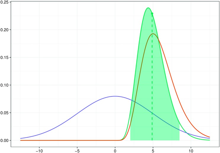
See Figure 1. This yields a coherent framework for estimation and uncertainty quantification based on the information encoded in the entire posterior probability distribution. For most realistic scenarios, the posterior is, however, not available in closed form. Inference is then typically based on samples drawn iteratively from the posterior using Markov chain Monte Carlo (MCMC) algorithms. For an introduction to Bayesian statistics, see Gelman et al. (2013).

Figure 1.

A graphical illustration of the Bayesian inferential regime: the prior (blue), the likelihood (red), and the posterior (green). The dotted line marks the posterior mean. The shaded region shows a 95% credible interval.

The Bayesian approach offers a few practical advantages over classical techniques. Typically, classical methods estimate the parameters by maximizing the data likelihood. Optimization methods may, however, not converge, especially in more complex models. The uncertainty of the estimates is usually assessed using asymptotic results. Bayesian methods, on the other hand, allow building complex models in a hierarchical fashion. MCMC algorithms try to stochastically explore the whole posterior probability space and hence are typically less prone to getting stuck at local optima, even in complex models. Point estimates of the parameters and their finite sample uncertainty estimates can be obtained directly out of the posterior samples. The posterior credible intervals (see Figure 1) also have actual probability interpretation, unlike frequentist confidence intervals.

In the next four sections, we describe the published speech learning experiment (Reetzke et al., 2018) used to demonstrate the utility of FLMEM. Then, the FLMEM is built in steps, starting with the linear mixed model. We first describe results on the speech learning experiment and then show the efficacy of the proposed method in a variety of simulated settings. Concluding remarks sum up the contributions of this work. Additional details, such as the MCMC algorithm to fit the model and so forth, are discussed in the Supplemental Materials.

Speech Learning Experiment

In a recent experiment, the timescale of sensory plasticity following speech learning in adulthood was assayed using electroencephalography paired with an extensive, individualized training paradigm (Reetzke et al., 2018). In this experiment, 20 native English-speaking adults were trained to categorize four Mandarin lexical tones: high-flat, Tone 1; low rising, Tone 2; low dipping, Tone 3; and high falling, Tone 4. On each trial of the experiment, participants listened to a lexical tone stimulus binaurally presented over Sennheiser HD 280 Pro circumaural headphones. Participants were instructed to categorize the stimulus into one of four categories by pressing number keys on a computer (1, 2, 3, or 4). Feedback was presented to the participant based on the accuracy of their response (“right” vs. “wrong”). Each individual participant was monitored until behavioral performance comparable to native Chinese Mandarin–speaking participants was achieved and maintained. Participants were then “overtrained” for an additional 10 days. Two months after training had ceased, participants returned to examine the extent to which learning was “retained.” The data presented here consist of learning curves of different lengths across 20 participants, as participants varied in the number of days it took them to reach native-like proficiency.

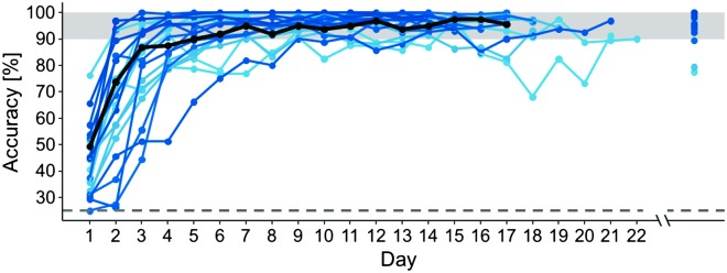
Reetzke et al. (2018) computed individual-level empirical estimates of the probabilities of success by counting the proportion of successes of each participant each time he or she was tested (see Figure 2). A large number of trials, n_i(t) = 180, were utilized to estimate these quantities with precision. The empirical estimates do not accommodate dependencies across adjacent time points or across estimates corresponding to the same individual. Naturally, the empirical probability curves cannot capture the expected smooth behavior of the underlying learning curves.

Figure 2.

Subject-by-day empirical learning curves (n = 20) from the speech training task. The gray region at the top shows the mean accuracy level, along with its standard error limits, for native Chinese participants (target criterion for learners); the dashed gray line at the bottom indicates accuracy of categorizing an input tone into one of four categories purely by random guess (25%). The emphasized black line shows the trajectory of a representative participant across time.

FLMEM

We use the data set from Reetzke et al. (2018) to illustrate different models and their relative advantages and disadvantages. Let y_i(t) be the number of successes obtained by the ith individual at time t in n_i(t) trials, where i = 1, …, n = 20 and t = 1, …, T = 17. In the speech learning experiment, the successes correspond to the correct identification of a presented Mandarin lexical tone as one of the four possible lexical tones. Letting the probability of success by the ith person at the tth time point be denoted by π_i(t), the trials to be independent, the total number of successes in n_i(t) trials follows a binomial distribution as

$$y_i\left(t\right)\mid {\pi }_i\left(t\right)\sim \mathit{Bin}\left\{n_i\left(t\right),{\pi }_i\left(t\right)\right\}.$$ (2)

We are interested in the population-level probability curve, denoted as π(t) sans any individual specific subscript, and how it evolves as the participants get trained over time. In addition, we want to estimate the individual learning curves π_i(t) and quantify their variability around the population baseline.

Linear Probability Models

One possible strategy to analyze the speech learning data may be via a linear mixed-effects model for the probabilities as

$${\pi }_i\left(t\right)={\beta }_0+{\beta }_{1}t+u_i,u_i\sim f_u\left(u_i\right).$$ (3)

Here, β₀ and β₁ are fixed regression coefficients, u_is are individual specific random effects distributed according the zero mean probability law f_u, typically assumed to be a normal distribution with variance ${\mathrm{\sigma }}_u^2$. The population-level average learning behavior is then obtained by integrating out the random effects from the individual-level mixed model as

$$\pi \left(t\right)=\int {\pi }_i\left(t\right)f_u\left(u_i\right)\mathrm{d}{u}_i={\beta }_0+{\beta }_{1}t.$$ (4)

Introducing artificial error terms ϵ_i(t), the linear mixed-effects model can be fitted to the empirical probability estimates plotted in Figure 2, henceforth denoted by ${\widehat{\pi }}_i\left(t\right)$, as

$${\widehat{\pi }}_i\left(t\right)={\beta }_0+{\beta }_{1}t+u_i+{ϵ}_i\left(t\right),$$ (5)

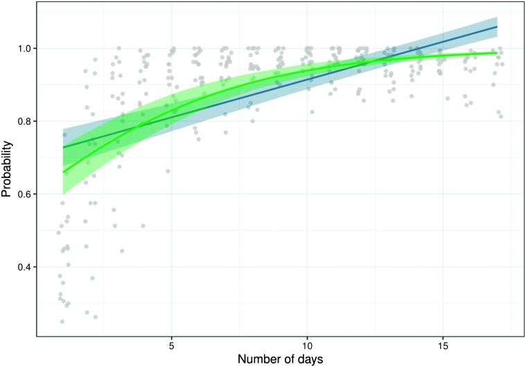
where ϵ_i(t) are error terms explaining the additional variations in ${\widehat{\pi }}_i\left(t\right)$, from the smooth linear curves π_i(t). Such practices are common in the current literature (Holt et al., 2018; Ingvalson et al., 2017; Moyle et al., 2007; Reetzke et al., 2018). Figure 3 shows the population-level estimate, fitting the above model to the sound-to-category data using the lme4 package in R.

Figure 3.

Population probability curve π(t) and its 95% confidence interval estimated by a linear mixed-effects model applied to the empirical success probabilities in the speech learning experiment (blue) superimposed over estimates obtained by fitting a logistic linear mixed-effects model (green).

The model clearly does not respect the restricted parameter space. Probabilities can only lie in the interval [0, 1]. The linear probability model suggests, however, with sufficiently large values of t, π(t) can be made larger than 1, and, for sufficiently small value of t, π(t) can be made even negative. In the sound-to-category data set, this actually happens well within the range of the observed time points.

Logistic Mixed-Effects Models

Generalized linear mixed models alleviate the limitations of linear probability models. The literature on generalized linear models, in particular logistic models, is enormous (Agresti, 2002; Cox, 1958; Cox & Snell, 1989; Dyke & Patterson, 1952). Jaeger (2008) provided an excellent review written for speech and language researchers. A logistic regression model can be viewed as a linear regression model, but on a transformed space. Specifically, in our longitudinal setting, a logistic mixed-effects model (LMEM) can be specified as

$$ln\frac{{\pi }_i\left(t\right)}{1-{\pi }_i\left(t\right)}={\beta }_0+{\beta }_{1}t+u_i,u_i\sim f_u\left(u_i\right).$$ (6)

The probability π_i(t) is then recovered from the model as

$${\pi }_i\left(t\right)=\frac{exp\left({\beta }_0+{\beta }_{1}t+u_i\right)}{1+exp\left({\beta }_0+{\beta }_{1}t+u_i\right)}=\frac{1}{1+exp\left(-{\beta }_0-{\beta }_{1}t-u_i\right)}.$$ (7)

The parameters π_i(t) are now always restricted to be in [0, 1] no matter how large or small t is. Logistic models are thus much better suited to model binomially distributed categorical data.

The population-level probabilities are obtained as before—by integrating out the random effects from the individual-level mixed model as

$$\pi \left(t\right)=\int {\pi }_i\left(t\right)f_u\left(u_i\right)\mathit{d}{u}_i=\int \frac{exp\left({\beta }_0+{\beta }_{1}t+u_i\right)}{1+exp\left({\beta }_0+{\beta }_{1}t+u_i\right)}{f}_u\left(u_i\right)\mathit{d}{u}_i.$$ (8)

Unlike the linear case, however, the above integral cannot be obtained in closed form for typical choices of random effects distributions, including the normal family (Wang & Louis, 2003). For conventional normally distributed random effects, an approximation is given in Zeger, Liang, and Albert (1988) as

$$\pi \left(t\right)=\int \frac{exp\left({\beta }_0+{\beta }_{1}t+u_i\right)}{1+exp\left({\beta }_0+{\beta }_{1}t+u_i\right)}\text{Normal}\left(u_i|0,{\sigma }_u^2\right)\mathrm{d}{u}_i\approx \frac{exp\left({\beta }_0^{\ast }+{\beta }_1^{\ast }t\right)}{1+exp\left({\beta }_0^{\ast }+{\beta }_1^{\ast }t\right)},$$ (9)

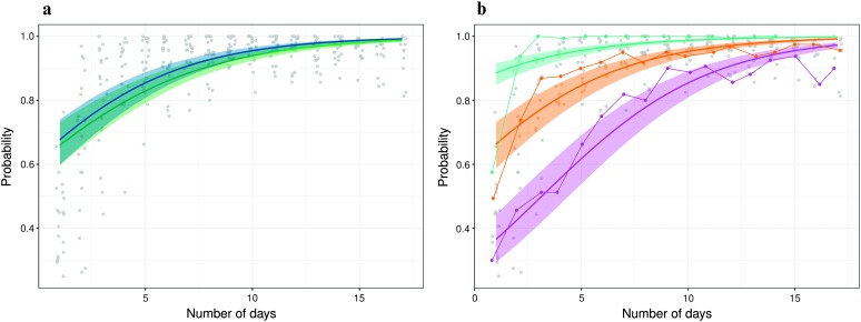
where ${\beta }_0^{\ast }={\beta }_0/{\left\{1+c^2{\sigma }_u^2\right\}}^{1/2}$ and ${\beta }_1^{\ast }={\beta }_1/{\left\{1+c^2{\sigma }_u^2\right\}}^{1/2}$ with $c=\left(16\sqrt{3}\right)/\left(15\pi \right)$. Without the correction, the population-level learning curve tends to get overestimated (see Figure 4a).

Figure 4.

(a) Estimated population probability curve π(t) by the logistic linear mixed-effects model (LMEM) method with (green) and without correction (blue). The shaded areas are the 95% confidence intervals for the mean function π(t). (b) Individual specific probability curves for three individuals and their 95% confidence intervals using the LMEM.

The LMEM, though a significant improvement over linear mixed models, is still very limited in its capacity to model widely varying learning curves. The assumption of linear regression on time cannot satisfy even in the logit-transformed scale. In the example speech learning experiment, for instance, the performances are generally poor at the beginning of the study and then improve rapidly, but never quite reach perfection. This hints at nonlinearity. A linear model on the logit scale typically implies that accuracy would rapidly reach 100%, as in Figure 4a. In particular, the LMEM significantly overestimates the probability of success in initial trials and then underestimates it for middle trials, eventually overestimating it again for the final trials. The estimates of the individual curves obtained by the LMEM method (see Figure 4b) also show similar behavior and are clearly heavily shape restricted. The probabilities in the early trials are again grossly overestimated. See, for example, the green and orange curves in Figure 4b. The opposite effect is seen, in particular in the violet curve, which is highly overestimated in the final trials. Mixed-effects models with higher degree polynomial terms can capture the residual variability, which is not explained by a simple first-degree linear model. It is not clear, however, how many terms should be included in such models. In the next section, we discuss how splines, specifically piecewise polynomial B-splines, can alleviate these problems by locally adapting to different smoothness patterns.

In addition, the individual heterogeneity may also vary over time. In the speech learning experiment, the performances of the participants were generally poor early in the study, and then their learning trajectories were quite varied during middle trials, eventually all attaining high success levels (because training was criterion dependent; see Figure 4b). The equal variance assumption, however, results in unrealistic uncertainty bounds around the estimates. The confidence bands are all very wide for the early trials even though empirical observation points to more homogeneous behavior in this phase of the experiment. They are also unrealistically narrow in the final trials.

FLMEMs

To alleviate these limitations, we propose a Bayesian model generalizing the LMEM to an FLMEM, that is,

$$ln\frac{{\pi }_i\left(t\right)}{1-{\pi }_i\left(t\right)}=\mu \left(t\right)+u_i\left(t\right).$$ (10)

The term μ(t) corresponds to the linear function β₀ + β₁ t in Equation 6, but it is now a flexible function of t, that is, a function that can adapt to different shapes other than linear. The terms u_i(t)s, corresponding to u_i in Equation 6, are additive individual specific effects as before, but now have the multiplicative structural form

$$u_i\left(t\right)=\xi \left(t\right){\eta }_i,{\eta }_i~\text{Normal}\left(0,{\sigma }_{\eta }^2\right),$$ (11)

where ξ(t) is another flexible function of t. This induces a time-varying variance for the random effects because $var\left\{u_i\left(t\right)\right\}={\sigma }_u^2\left(t\right)=\xi {\left(t\right)}^2{\sigma }_{\eta }^2$. This multiplicative parameterization of the random effects is a functional version of the “parameter expanded” model (Liu & Wu, 1999; van Dyk & Meng, 2001), originally introduced to reduce dependence among the parameters in a hierarchical model and to improve MCMC convergence. A time-varying variance is important in order to model latent heterogeneity among participants that can increase or decrease during the study. The model described here has similarities with the functional mixed-effects model proposed in Guo (2002) and a generalization presented in Kliethermes and Oleson (2014). The latter adopted a less statistically principled approach, introducing artificial errors to make computation simpler while also using somewhat ad hoc random effects structure.

As in the case of LMEM, the population-level learning curve is obtained as

$$\pi \left(t\right)=\int \frac{exp\left\{\mu \left(t\right)+u_i\left(t\right)\right\}}{1+exp\left\{\mu \left(t\right)+u_i\left(t\right)\right\}}\text{Normal}\left(u_i|0,\xi {\left(t\right)}^2{\sigma }_{\eta }^2\right)\mathrm{d}{u}_i\approx \frac{exp\left\{{\mu }^{\ast }\left(t\right)\right\}}{1+exp\left\{{\mu }^{\ast }\left(t\right)\right\}},$$ (12)

where ${\mu }^{\ast }\left(t\right)=\mu \left(t\right)/{\left\{1+c^2\xi {\left(t\right)}^2{\sigma }_{\eta }^2\right\}}^{1/2}$ with $c=\left(16\sqrt{3}\right)/\left(15\pi \right)$.

We now focus on modeling the functions μ(t) and ξ(t) flexibly. In this work, we use weighted mixtures of quadratic B-splines to model a generic function f(t) as $f\left(t\right)={\sum }_{j=1}^J{b}_{q,j}\left(t\right){\beta }_j$. Consider positive integers K and q, denoting the number of intervals and the spline degree, respectively. Partition a compact interval [a, b] into K subintervals defined by knot points a = t ₁ = ⋯ = t _q+1 < t _q+2 < ⋯ < t _q+K < t _q+K+1 = ⋯ = t _2q+K+1 = b. One can then construct J = q + K spline basis functions of degree q, denoted by B _q,J(t) = {b _q,1(t), …, b _q,J(t)}^T through a recursion relation given in de Boor (1978). See Supplemental Material S2 for an illustration of quadratic (q = 2) basis functions. The B-splines satisfy a local support property. Specifically, b_q,j(t) is supported only on [t_j, t _j+q+1]. This means flexible functions $f\left(t\right)={\sum }_{j=1}^J{b}_{q,j}\left(t\right){\beta }_j$ can be modeled by varying the spline coefficients β = (β₁, …, β_J)^T. Large (positive or negative) values of β_j will lead to large (positive or negative) values of f(t) on the local support of the associated spline basis b_q,j(t). Likewise, similar successive values of β_j will result in a flat region in f(t). See Supplemental Material S3 for an illustration.

We thus model μ(t) flexibly with a mixture of B-splines as

$$\mu \left(t\right)=\sum _{j=1}^J{b}_{q,j}\left(t\right){\beta }_j.$$ (13)

As mentioned in the introduction, we adopt a Bayesian route to fit the FLMEM, assigning each parameter a prior and inferring them from the posterior. The spline coefficients are assigned the smoothness-inducing prior

$$\begin{array}{l}\mathbf{\beta }\mid {\sigma }_{\beta }^2\sim {\mathrm{MVN}}_J\left(\mathbf{0},{\sigma }_{\beta }^2{\mathit{P}}^{-1}\right)\\ {\sigma }_{\beta }^2\sim \mathrm{Inv}-\mathrm{Ga}\left(a_{\beta },b_{\beta }\right).\end{array}$$ (14)

Here, MVN_J(μ, P ⁻¹) denotes a J-dimensional multivariate normal distribution with mean μ and precision P; Inv − Ga(a, b) denotes an inverse gamma distribution with shape parameter a and rate parameter b. Also, P = D ^T D, where the (J − 2) × J matrix D is such that Dβ computes the second differences in β. This prior thus penalizes ${\sum }_{j=1}^J{\left({\nabla }^2{\beta }_j\right)}^2={\mathbf{\beta }}^{\mathit{T}}\mathit{P}\mathbf{\beta }$, the sum of squares of second-order differences in β (Eilers & Marx, 1996) and thus makes the function smooth. The variance parameter ${\mathrm{\sigma }}_{\beta }^2$ is the smoothness-inducing parameter—the smaller the value of ${\mathrm{\sigma }}_{\beta }^2$, the stronger the penalty and the smoother the function. It is assigned an inverse Gamma hyperprior and inferred from the data. The smoothness of the underlying function is thus data adaptive and not fixed in advance. Analogously, we model ξ(t) as

$$\mathrm{\xi }\left(t\right)=\sum _{j=1}^J{b}_{q,j}\left(t\right){\mathrm{\gamma }}_i,\mathbf{\gamma }\mid {\mathrm{\sigma }}_{\mathrm{\gamma }}^2\sim {\mathrm{MVN}}_J\left(\mathbf{0},{\mathrm{\sigma }}_{\mathrm{\gamma }}^2{\mathit{P}}^{-1}\right),{\sigma }_{\gamma }^2\sim \mathrm{Inv}-\mathrm{Ga}\left(a_{\gamma },b_{\gamma }\right).$$ (15)

Therefore, the fixed and random functional effects are modeled in the same functional space (Guo, 2002). For the variance of the random effects components η_i,, we specify the prior

$${\mathrm{\sigma }}_{\mathrm{\eta }}^2\sim \mathrm{Inv}-\mathrm{Ga}\left(\frac{a_{\mathrm{\eta }}}{2},\frac{a_{\mathrm{\eta }}}{2}\right).$$ (16)

The computational strategy to fit the model is based on the Pòlya-Gamma scheme proposed in Polson, Scott, and Windle (2013). For the two smoothing parameters ${\mathrm{\sigma }}_{\beta }^2$ and ${\mathrm{\sigma }}_{\mathrm{\gamma }}^2$, the prior is noninformative for small values of their hyperparameters. Thus, we set a _β = b _β = a _γ = b _γ = 0.5. Similarly, for the prior on ${\mathrm{\sigma }}_{\eta }^2$, we use a _η = 0.5. The algorithm converges rapidly to the stationary distribution for all of the parameters. Convergence and stationarity of the chain were assessed by examining trace plots and using the Geweke diagnostic criterion (Geweke, 1992). Further details are deferred to Supplemental Material S1. Moreover, a sensitivity analysis on the hyperparameters has been performed, and similar results were achieved.

We programmed in R interfaced with C++. In each case, 7,500 MCMC iterations were run with the initial 2,500 iterations discarded as burn-in. For n = 20 and n_i(t) = 80 for all i and all t, the computation time is less than 2 min. An R package implementing our method, including an instruction manual and demos, is available in the Supplemental Materials.

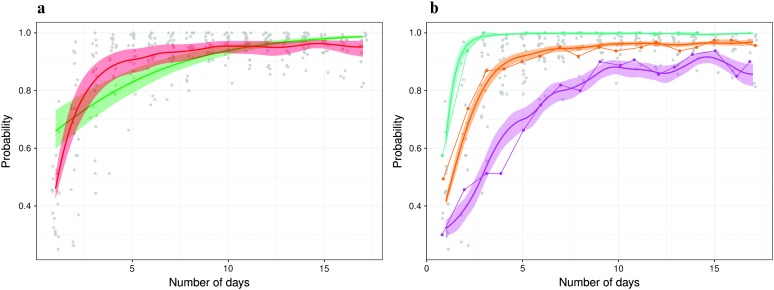
Figures 5, 6, and 7 summarize the results of the FLMEM applied to the speech learning data. The population learning curve π(t) estimated by the FLMEM looks very different from the estimate obtained by the LMEM (see Figure 5a). Being severely shape restricted, the LMEM did not capture the rapid improvements early on and also the plateaued performances later in the study. The FLMEM, on the other hand, provides more realistic estimates, capturing well the empirically observed patterns. On Day 1, for example, the FLMEM estimates the population-level average success probability at π(t) = 0.45, whereas the LMEM estimated it at 0.65—a difference of 0.20. The FLMEM estimates quickly surpass the LMEM, and on Day 4, the estimates by the FLMEM and the LMEM are approximately 0.80 and 0.90, respectively. Finally, on Day 17, the estimates by the FLMEM and the LMEM are 0.95 and 0.99, respectively. The estimates of individual learning curves (see Figure 5b) have also greatly improved (compare with Figure 4b), illustrating the flexibility of the FLMEM in adapting to varying shapes.

Figure 5.

(a) Estimated population probability curves π(t). The solid lines represent the estimates according to the logistic linear mixed-effects model (green) and the functional logistic mixed-effects model (FLMEM; red). The shaded areas are the 95% credible/confidence intervals for the mean function π(t). (b) Individual specific probability curves for three individuals and their 95% credible intervals, obtained using the FLMEM.

Figure 6.

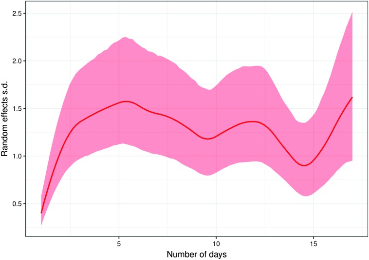
The random effects standard deviation σ_u(t) and its 95% credible intervals.

Figure 7.

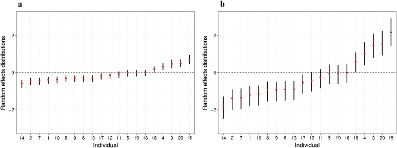
Posterior means (red dots) and 95% credible intervals (black lines) of the random effects u_i arranged in increasing order of magnitude at time t = 1 (a) and t = 10 (b).

The random effect variance is also not constant but varies over time (see Figure 6). Figure 7 shows the estimated random effects on Days 1 and 10 of the trials. These figures provide strong evidence that the latent heterogeneity is small early on but increases later, which, in turn, has resulted in more realistic uncertainty bounds around the estimates.

It is worth noting that the proposed model can be reformulated as a traditional linear mixed-effects model. See details in the Supplemental Materials. We could thus try to fit these models using a frequentist approach implemented in the lme4 package in R. Our experience with such attempts suggests that they cannot converge, even in the simpler LMEM case. The Bayesian approach and its MCMC-based implementation, on the other hand, always converged, providing very stable estimates of the parameters and their uncertainties.

Testing

We may also be interested in formally testing various hypotheses related to the behavior of the learning curves, such as the extent to which (a) there is a significant difference in the population curve between two specific points in time, (b) if an individual performs significantly differently at a two specific time points, or (c) if two individuals perform significantly differently at a specific time point. For the testing problem (a) above, θ = π(t ₁)−π(t ₂), whereas for (b), θ = π_i(t ₁)−π_i(t ₂), and for (c), θ = π_i(t ₁)−π_j(t ₁) for individuals i and j. Following Berger and Delampady (1987), we can represent the problems generically as $H_0^{\mathrm{ϵ}}=\left|\theta \right|<\mathrm{ϵ}$ versus $H_1^{\mathrm{ϵ}}=\left|\mathrm{\theta }\right|>\mathrm{ϵ}$, where θ is the difference of interest and ϵ represents its practical limits of significance. MCMC-based implementation of our Bayesian method provides us with samples of the individual curves and the population curve. The posterior distributions of the difference between curves at particular time points are thus readily available from the MCMC output, so are the estimates of the posterior probabilities, $p\left(H_0^{\mathrm{ϵ}}|\text{data}\right)$. Specifically, we have $p\left(H_0^{ϵ}|\text{data}\right)=\frac{1}{G}{\sum }_g\mathbb{I}\left\{{\mathrm{\theta }}^{\left(g\right)}ϵ\left[-ϵ,ϵ\right]\right\}$, where G is the number of MCMC iterations and θ^(ɡ) is the sampled values at iteration ɡ. We reject $H_0^{ϵ}$ if p(H ₀|data) < α, a chosen level of significance.

As a numerical example, say we are interested in testing the extent to which, in our sound to category experiment, the population curve is significantly different between the time points t ₁ = 1 and t ₂ = 5 and then between t ₂ = 5 and t ₃ = 10 (see Figure 5a) with ϵ = 0.05. The probability $p\left(H_0^{ϵ}|\text{data}\right)$ is then 0 in the first case and 0.626 in the second one, leading to rejection of the null hypothesis in the first test but a failure to reject in the latter.

Simulation Experiments

To illustrate the efficacy of the FLMEM in efficiently recovering the population and individual-level learning curves in general settings, we designed a simulation study comparing its performance with two popular models: the LMEM and the LMEM+ (with higher order terms up to the fourth order), both implemented using the glmer function of the lme4 R package (Bates, Maechler, Bolker, & Walker, 2014). In both models, we used random effects for both intercept and slope. That is, we fitted the model ln[π_i(t)/{1−π_i(t)}] = β₀ + β₁ t + γ_0i +γ_1i t for the linear case and ln[π_i(t)/{1−π_i(t)}] = β₀ + β₁ t + β₂ t ² + β₃ t ³ + β₄ t ⁴ + γ_0i + γ_1i t for the polynomial case.

We simulated n = 20 learning curves at T = 20 time points with n_i(t) = 40 trials under eight possible scenarios, with four possible choices for the true underlying function μ(t) and two possible choices for ξ(t). In particular, for μ(t), we tried (a) a linear function μ(t) = −2 + 0.7t, (b) a quadratic function μ(t) = −1 + 0.02t ², (c) a step function μ(t) = −2 ⋅ 𝕀{t < 7.5} + 0.5 ⋅ 𝕀{7.5 ≤ t < 12.5} + 5 ⋅ 𝕀{t ≥ 12.5}, and (d) an oscillatory function μ(t) = −2 + 0.5 t + 0.5 sin(t). For ξ(t), we tried (a) a constant ξ(t) = 1 and (b) a linear ξ(t) = 0.5 + 0.224 t function. In all the experiments, we set the true σ_η to be 0.8.

As a metric of goodness-of-fit, we measure how well the population-level learning curve π(t) is recovered. In particular, we use the mean integrated squared error (MISE). The MISE for estimating f(t) by $\widehat{f}\left(t\right)$ is defined as

$$\text{MISE}=\mathbb{E}\left[\int {\left\{f\left(t\right)-\widehat{f}\left(t\right)\right\}}^2\mathrm{d}t\right].$$ (17)

We estimate the MISE by averaging the estimated integral across B simulated data sets as ${\text{MISE}}_{\mathit{est}}=\frac{1}{B}{\sum }_{b=1}^B{\sum }_{i=1}^N{\mathrm{\Delta }}_i{\left\{f\left(t_i\right)-\widehat{f}\left(t_i\right)\right\}}^2$, where Δ_i = t_i−t _i−1 and ${\left\{t_i\right\}}_{i=1}^N$ are a set of grid points on the range of the data. In Table 1, the reported estimated MISEs are based on B = 50 simulated data sets.

Table 1.

Mean integrated squared error (MISE) between the true population function π(t) and the estimated population function π(t) estimated by the two models under different scenarios.

True π(t)	True ξ(t)	MISE × 103
		LMEM	LMEM+	FLMEM
1	(a)	0.35	0.37	0.45
	(b)	0.13	0.14	0.80
2	(a)	2.73	0.93	0.94
	(b)	2.57	0.80	1.02
3	(a)	10.42	9.21	0.77
	(b)	9.85	9.58	0.63
4	(a)	2.27	1.45	0.74
	(b)	2.09	1.27	0.45

Note. Bold text denotes the models that are significantly outperforming the others in each simulation scenario (see Supplemental Material S4 for further details). LMEM = logistic linear mixed-effects model; LMEM+ = logistic mixed-effects models with higher order terms; FLMEM = functional logistic mixed-effects models.

In Table 1, one can see that FLMEM performs competitively in comparison with logistic mixed-effects models (LMEM) or LMEM+ even when the ground truth is linear or quadratic. Moreover, as discussed throughout this article, linearity is a highly unrealistic assumption for most practical applications. In general, for nonlinear cases not corresponding to simple polynomials, the FLMEM vastly outperforms both the LMEM and the LMEM+. Supplemental Material S4 reports the distributions of the ISEs under the eight possible scenarios.

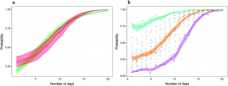
Figures 8 and 9 correspond to the Simulation Scenario 2(a). In Figure 8a, the estimate of the population learning curve π(t) is shown. For this example, data were generated from an underlying quadratic function, and therefore, we expect the FLMEM model to outperform the simpler LMEM. The fit obtained via lme4 is, unsurprisingly, poor. On the other hand, our model recovers the true population learning curve very efficiently. In Figure 8b, three individual specific probability curves are displayed. Let us remind the reader that we are comparing confidence intervals of the simpler models LMEM and LMEM+ (obtained via bootstrap using glmer) with credible intervals obtained from the MCMC samples in the case of FLMEM. This is necessary because the methods used to fit these models are different (frequentist for the former, Bayesian for the latter).

Figure 8.

Results for simulated data. (a) Estimated population probability curves π(t) superimposed over the truth (blue dashed line). The solid lines represent the estimates according to the logistic linear mixed-effects model (green) and the functional logistic mixed-effects model (FLMEM; red). The shaded areas are the 95% credible/confidence intervals for the mean function π(t). (b) Individual specific probability curves for three individuals and their 95% credible intervals, obtained using the FLMEM.

Figure 9.

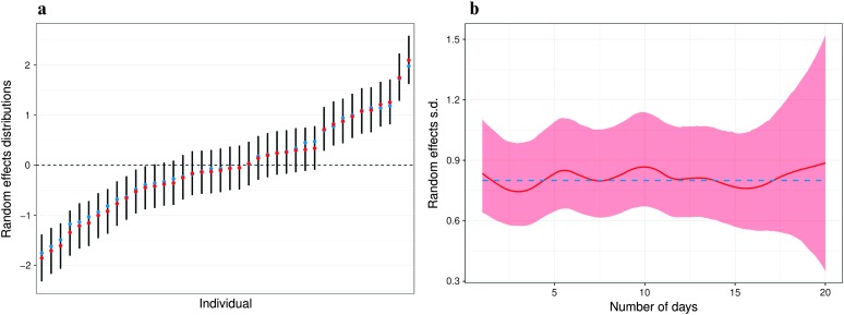
Results for simulated data. (a) Posterior means (red dots) and 95% credible intervals of the random effects u_i at t = 1, arranged in increasing order of magnitude. (b) Marginal posterior distribution for the random effects standard deviation σ_u(t) and its credible intervals. The blue dashed line represents the true value.

Figure 9a shows the random effects posterior distributions at the initial time t = 1. In Figure 9b, we report the posterior distribution for the standard deviation of the random effects as a function of time. Using a constant random effect variance, we expect our model to recover the true flat variance function σ_u = |ξ(t)|σ_η = σ_η. As we can see, the estimated function σ_u(t) is flat, and its mean is coherently close to σ_u. The loss of accuracy for large values of t can be explained by the fact that, in that region, μ(t) is large. Therefore, larger values of u_i could yield to the same implied probability of ≈1.

Discussion

The current state of the art in speech, language, and hearing research for modeling data over various time points is primarily dominated by linear and logistic mixed-effects models. Traditional linear and logistic mixed-effects models assume linearity in the observed or transformed logit scales and also assume the random effects heterogeneity to remain constant over time. We presented an approach, namely, FLMEM, that relaxes these limitations by allowing more flexible regression and variance models in the transformed scale using smoothed mixture of B-splines. Moreover, the Bayesian estimation procedure outlined in this article allows a coherent framework for finite sample estimation and uncertainty quantification.

We demonstrated the utility of the proposed FLMEM in estimating learning curves using data from a recent speech learning study and via a simulation experiment. Specifically, we showed that the FLMEM is more flexible and efficient in estimating individual- and population-level learning curves across different time points relative to linear and generalized linear mixed-effects models.

The methods described here are broadly applicable to speech, language, and hearing experiments wherein repeated measures are collected from participants over time, for example, not only in learning experiments (as demonstrated here) but also in treatment paradigms, where the focus is to capture both individual- and group-level treatment gains over time (Anderson et al., 2014, 2013; Burk & Humes, 2008). In the current article, we show that FLMEM, when compared to linear and generalized linear mixed-effects models, recovers the true population and the individual-level learning curves and therefore may be very useful for meeting the goals of future researchers. In particular, as we have a better understanding of sources of individual differences, there is potential toward personalized approaches to learning. Such applications necessitate to accurately estimate the population and single individuals, and we expect that our model is well suited to take on the complexities of personalized approaches.

Ongoing directions of research include the simultaneous modeling of success probabilities for each of the different input tones, as well as the accommodation of exogenous covariates. These directions would allow us to understand the learning process separately for the four phonemes at a much deeper level than what is possible using existing methods. Moreover, it is possible to incorporate exogenous covariates in the model, as well as clustering curves into homogeneous latent subgroups and so forth.

Funding Statement

This work was supported by the National Institute on Deafness and Other Communication Disorders Grants R01DC013315 and R01DC015504, awarded to Chandrasekaran. The content does not necessarily represent the official views of the National Institutes of Health.

References

- Agresti A. (2002). Categorical data analysis (2nd ed.). New York, NY: Wiley-Interscience. [Google Scholar]
- Anderson S., White-Schwoch T., Choi H. J., & Kraus N. (2014). Partial maintenance of auditory-based cognitive training benefits in older adults. Neuropsychologia, 62, 286–296. [DOI] [PMC free article] [PubMed] [Google Scholar]
- Anderson S., White-Schwoch T., Parbery-Clark A., & Kraus N. (2013). Reversal of age-related neural timing delays with training. Proceedings of the National Academy of Sciences, 110(11), 4357–4362. [DOI] [PMC free article] [PubMed] [Google Scholar]
- Bates D., Maechler M., Bolker B., & Walker S. (2014). Package lme4: Linear-mixed effects models using Eigen and S4. R Package Version 67.
- Berger J., & Delampady M. (1987). Testing precise hypotheses. Statistical Science, 3, 317–352. [Google Scholar]
- Bialystok E., Luk G., Peets K. F., & Yang S. (2010). Receptive vocabulary differences in monolingual and bilingual children. Bilingualism: Language and Cognition, 13(4), 525–531. [DOI] [PMC free article] [PubMed] [Google Scholar]
- Burk M. H., & Humes L. E. (2008). Effects of long-term training on aided speech-recognition performance in noise in older adults. Journal of Speech, Language, and Hearing Research, 51(3), 759–771. [DOI] [PMC free article] [PubMed] [Google Scholar]
- Cox D. R. (1958). The regression analysis of binary sequences. Journal of the Royal Statistical Society. Series B (Methodological), 20(2), 215–242. [Google Scholar]
- Cox D. R., & Snell E. J. (1989). Analysis of binary data (2nd ed.). London, United Kingdom: Chapman & Hall. [Google Scholar]
- de Boor C. (1978). A practical guide to splines (Vol. 27, 1st ed.). New York, NY: Springer-Verlag. [Google Scholar]
- Dyke G. V., & Patterson H. D. (1952). Analysis of factorial arrangements when the data are proportions. Biometrics, 8(1), 1–12. [Google Scholar]
- Eilers P. H. C., & Marx B. D. (1996). Flexible smoothing with B-splines and penalties. Statistical Science, 11(2), 89–121. [Google Scholar]
- Gelman A., Stern H. S., Carlin J. B., Dunson D. B., Vehtari A., & Rubin D. B. (2013). Bayesian data analysis (3rd ed.). New York, NY: Chapman & Hall/CRC. [Google Scholar]
- Geweke J. (1992). Evaluating the accuracy of sampling-based approaches to calculating posterior moments. In Bernardo J. M., Berger J. O., Dawid A. P., & Smith A. F. M. (Eds.), Bayesian Statistics 4 (pp. 169–193). Oxford, England: Oxford University Press. [Google Scholar]
- Guo W. (2002). Functional mixed effects models. Biometrics, 58(1), 121–128. [DOI] [PubMed] [Google Scholar]
- Holt C. M., Lee K. Y. S., Dowell R. C., & Vogel A. P. (2018). Perception of Cantonese lexical tones by pediatric cochlear implant users. Journal of Speech, Language, and Hearing Research, 61(1), 1–12. [DOI] [PubMed] [Google Scholar]
- Ingvalson E. M., Lansford K. L., Fedorova V., & Fernandez G. (2017). Receptive vocabulary, cognitive flexibility, and inhibitory control differentially predict older and younger adults' success perceiving speech by talkers with dysarthria. Journal of Speech, Language, and Hearing Research, 60(12), 3632–3641. [DOI] [PubMed] [Google Scholar]
- Jaeger T. F. (2008). Categorical data analysis: Away from ANOVAs (transformation or not) and towards logit mixed models. Journal of Memory and Language, 59(4), 434–446. [DOI] [PMC free article] [PubMed] [Google Scholar]
- Jia G. (2003). The acquisition of the English plural morpheme by native Mandarin Chinese–speaking children. Journal of Speech, Language, and Hearing Research, 46(6), 1297–1311. [DOI] [PubMed] [Google Scholar]
- Kliethermes S., & Oleson J. (2014). A Bayesian approach to functional mixed-effects modeling for longitudinal data with binomial outcomes: Functional mixed-effects modeling for longitudinal binomial outcomes. Statistics in Medicine, 33(18), 3130–3146. [DOI] [PMC free article] [PubMed] [Google Scholar]
- Lairdl N. M., & Ware J. H. (1982). Random-effects models for longitudinal data. Biometrics, 963–974. [PubMed] [Google Scholar]
- Liu J. S., & Wu Y. N. (1999). Parameter expansion for data augmentation. Journal of the American Statistical Association, 94(448), 1264–1274. [Google Scholar]
- Morris J. S. (2015). Functional regression. Annual Review of Statistics and Its Application, 2(1), 321–359. [Google Scholar]
- Moyle M. J., Ellis Weismer S., Evans J. L., & Lindstrom M. J. (2007). Longitudinal relationships between lexical and grammatical development in typical and late-talking children. Journal of Speech, Language, and Hearing Research, 50(2), 508–528. [DOI] [PMC free article] [PubMed] [Google Scholar]
- Pearson B. Z., Fernández S. C., & Oller D. K. (1993). Lexical development in bilingual infants and toddlers: Comparison to monolingual norms. Language Learning, 43(1), 93–120. [Google Scholar]
- Polson N. G., Scott J. G., & Windle J. (2013). Bayesian inference for logistic models using Pólya-Gamma latent variables. Journal of the American Statistical Association, 108(504), 1339–1349. [Google Scholar]
- Ramsay J., & Silverman B. W. (1997). Functional data analysis (1st ed.). New York, NY: Springer-Verlag. [Google Scholar]
- Reetzke R., Xie Z., Llanos F., & Chandrasekaran B. (2018). Tracing the trajectory of sensory plasticity across different stages of speech learning in adulthood. Current Biology, 28(9), 1419–1427. [DOI] [PMC free article] [PubMed] [Google Scholar]
- Rice J. A., & Silverman B. W. (1991). Estimating the mean and covariance structure nonparametrically when the data are curves. Journal of the Royal Statistical Society. Series B (Methodological), 53(1), 233–243. [Google Scholar]
- Uccelli P., & Páez M. M. (2007). Narrative and vocabulary development of bilingual children from kindergarten to first grade: Developmental changes and associations among English and Spanish skills. Language, Speech, and Hearing Services in Schools, 38(3), 225–236. [DOI] [PMC free article] [PubMed] [Google Scholar]
- van Dyk D. A., & Meng X.-L. (2001). The art of data augmentation. Journal of Computational and Graphical Statistics, 10(1), 1–50. [Google Scholar]
- Wang Z., & Louis T. A. (2003). Matching conditional and marginal shapes in binary random intercept models using a bridge distribution function. Biometrika, 90(4), 765–775. [Google Scholar]
- Warton D. I., & Hui F. K. C. (2011). The arcsine is asinine: The analysis of proportions in ecology. Ecology, 92(1), 3–10. [DOI] [PubMed] [Google Scholar]
- Wong P. C., Perrachione T. K., & Parrish T. B. (2007). Neural characteristics of successful and less successful speech and word learning in adults. Human Brain Mapping, 28(10), 995–1006. [DOI] [PMC free article] [PubMed] [Google Scholar]
- Zatorre R. J. (2013). Predispositions and plasticity in music and speech learning: Neural correlates and implications. Science, 342(6158), 585–589. [DOI] [PubMed] [Google Scholar]
- Zeger S. L., Liang K.-Y., & Albert P. S. (1988). Models for longitudinal data: A generalized estimating equation approach. Biometrics, 44(4), 1049–1060. [PubMed] [Google Scholar]
Associated Data
This section collects any data citations, data availability statements, or supplementary materials included in this article.