

Abstract
New species arise from pre-existing species and inherit similar genomes and environments. This predicts greater similarity of the tempo of molecular evolution between direct ancestors and descendants, resulting in autocorrelation of evolutionary rates in the tree of life. Surprisingly, molecular sequence data have not confirmed this expectation, possibly because available methods lack the power to detect autocorrelated rates. Here, we present a machine learning method, CorrTest, to detect the presence of rate autocorrelation in large phylogenies. CorrTest is computationally efficient and performs better than the available state-of-the-art method. Application of CorrTest reveals extensive rate autocorrelation in DNA and amino acid sequence evolution of mammals, birds, insects, metazoans, plants, fungi, parasitic protozoans, and prokaryotes. Therefore, rate autocorrelation is a common phenomenon throughout the tree of life. These findings suggest concordance between molecular and nonmolecular evolutionary patterns, and they will foster unbiased and precise dating of the tree of life.
Keywords: TimeTree, rate autocorrelation, phylogenomics
Introduction
Rates of molecular sequence evolution vary extensively among species (Ho and Duchêne 2014; Dos Reis et al. 2016; Kumar and Hedges 2016). The causes and consequences of evolutionary rate variation among species are of fundamental importance in molecular phylogenetics and systematics (Kimura 1983; Lanfear et al. 2010; Lynch 2010). They inform about the relationship among molecular, biological, and life history traits and are a prerequisite for reliable estimation of divergence times among species and genes (Ho and Duchêne 2014; Kumar and Hedges 2016).
Three decades ago, Gillespie (1984) proposed that molecular evolutionary rates within a phylogeny will be autocorrelated due to similarities in genomes, biology, and environments between ancestral species and their immediate progeny. This idea led to statistical modeling of the variability of evolutionary rates among branches and formed the basis of the earliest methods for estimating divergence times without assuming a strict molecular clock (Sanderson 1997; Thorne et al. 1998; Kumar 2005; Ho and Duchêne 2014; Kumar and Hedges 2016). However, the independent branch rate (IBR) model has emerged as a strong alternative to the autocorrelated branch rate (ABR) model. The IBR model posits that rates vary randomly throughout the tree, such that the evolutionary rate similarity between an ancestor and its descendant is, on average, no more than that between more distantly related branches in a phylogeny (Drummond et al. 2006; Ho and Duchêne 2014).
The IBR model is now widely used in estimating divergence times from molecular data for diverse groups of species. It has been assumed for mammals (Drummond et al. 2006), birds (Brown et al. 2008; Claramunt and Cracraft 2015; Prum et al. 2015), amphibians (Feng et al. 2017), plants (Moore and Donoghue 2007; Bell et al. 2010; Smith et al. 2010; Linder et al. 2011; Lu et al. 2014; Barreda et al. 2015; Barba-Montoya et al. 2018), and viruses (Drummond et al. 2006; Buck et al. 2016; Metsky et al. 2017). If the IBR model best explains the variability of evolutionary rates, then we must infer a decoupling of molecular and biological evolution. This is because morphology, behavior, and other life history traits are more similar between closely related species (Sargis and Dagosto 2008; Lanfear et al. 2010; Cox and Hautier 2015) and are correlated with taxonomic or geographic distance (Wyles et al. 1983; Shao et al. 2016).
Alternatively, the widespread use of the IBR model (Drummond et al. 2006; Moore and Donoghue 2007; Brown et al. 2008; Bell et al. 2010; Smith et al. 2010; Linder et al. 2011; Lu et al. 2014; Claramunt and Cracraft 2015; Prum et al. 2015; Buck et al. 2016; Feng et al. 2017; Metsky et al. 2017) may be due to the fact that the currently available statistical tests lack sufficient power to reject the IBR model (Ho et al. 2015). In fact, some studies report extensive branch rate autocorrelation (e.g., Lepage et al. 2007), but others do not agree (e.g., Linder et al. 2011).
Consequently, many researchers use both ABR and IBR models when applying Bayesian methods to date divergences (Wikström et al. 2001; Drummond et al. 2006; Bell et al. 2010; Erwin et al. 2011; Meredith et al. 2011; dos Reis et al. 2012, 2015, 2018; Magallón et al. 2013; Jarvis et al. 2014; Hertweck et al. 2015; Foster et al. 2016; Liu et al. 2017; Pacheco et al. 2018; Takezaki 2018). This practice can result in widely differing time estimates under ABR and IBR models, which makes biological interpretation challenging (Battistuzzi et al. 2010; Christin et al. 2014; Dos Reis et al. 2014, 2015; Foster et al. 2016; Liu et al. 2017; Pacheco et al. 2018; Takezaki 2018). For example, as compared with the ABR model, the use of IBR model has been reported to produce 66% older estimates of divergence times for two major groups of grasses (Christin et al. 2014), 30% older divergence estimate for the origin of a major group of mammal (Erinaceidea) (Meredith et al. 2011), and 50% younger estimates for two clades of parasitic protozoans in birds (Pacheco et al. 2018). The choice of branch rate model also strongly influences posterior credibility intervals, because these intervals are often wider under the ABR model (Battistuzzi et al. 2010).
Therefore, we need a powerful method to accurately test whether evolutionary rates are autocorrelated in a phylogeny. Application of this method to molecular data sets representing taxonomic diversity across the tree of life will enable an assessment of the preponderance of autocorrelated rates in nature. Here, we introduce a new machine learning (McL) approach (CorrTest) that shows high power to detect autocorrelation between molecular branch rates. CorrTest is computationally efficient, and its application to a large number of data sets establishes the pervasiveness of rate autocorrelation in the tree of life.
New Method
McL is widely used to solve problems in many fields, including ecology (Christin et al. 2018; Willcock et al. 2018) and population genetics (Saminadin-Peter et al. 2012; Schrider and Kern 2016; Schrider and Kern 2018). We present a supervised McL framework (Bzdok et al. 2018) used to build a predictive model that distinguishes between ABR and IBR models, a major challenge in molecular phylogenetics and phylogenomics. In our McL approach, the input is a molecular phylogeny with branch lengths and the output is a classification that corresponds to whether or not the evolutionary rates in the phylogeny are autocorrelated among branches (ABR or IBR, respectively). An overview of our McL approach is presented in figure 1.
Fig. 1.

A flowchart showing an overview of the McL approach applied to develop the predictive model (CorrTest). We generated (a) 1,000 training data sets that were simulated using IBR models and (b) 1,000 training data sets that were simulated using ABR models. The numerical state (c) for all IBR data sets was 0 and (d) for all ABR data sets was 1. For each data set, we estimated a molecular phylogeny with branch lengths (e and f) and computed ρs, ρad, d1, and d2 (g and h) that served as features during the supervised McL. (i) Supervised McL was used to develop a predictive relationship between the input features and numerical states. (j) The predictive model produces a CorrScore for an input phylogeny with branch lengths. The predictive model was (k) validated with 10- and 2-fold cross-validation tests, (l) tested using external simulated data, and then (m) applied to empirical data to examine the prevalence of rate autocorrelation in the tree of life.
To build a predictive model, McL needs measurable properties (features) that can be derived from the input data (phylogeny with branch lengths). The selection of informative and discriminating features (fig. 1g and h) is critical to the success of McL. We derive relative lineage rates using a given molecular phylogeny with branch (“edge”) lengths (fig. 1e and f) by using Tamura et al.’s (2018) method and use these relative rates to generate informative features. The use of the relative rate framework (RRF) is necessary because we cannot derive branch rates without knowing node times in the phylogeny. For example, we need to know node times ti’s in figure 2 to convert branch lengths into branch rates, but these node times are what investigators wish to estimate by using a Bayesian approach that requires selection of a branch rate model. In contrast, the estimation of relative lineage rates does not require knowledge of divergence times. This is because an evolutionary lineage includes all the branches in the descendant subtree (e.g., lineage a contains branches with lengths b1, b2, and b5 in fig. 2) and the relative rate between sister lineages is simply the ratio of the evolutionary depths of the two lineages (Tamura et al. 2018). In figure 2, Ra and Rb are two lineage rates whose relative value can be estimated by the ratio of lineage lengths La and Lb, where the lineage length is a function of lengths of all branches in the subtree. Tamura et al. (2018) presented RRF to estimate these relative lineage rates analytically by using branch lengths only. Furthermore, Tamura et al.’s (2018) method generates relative lineage rates such that all the lineage rates in a phylogeny are relative to the rate of the ingroup root lineage (R0, fig. 2). Use of RRF enabled us to develop a number of features for building a McL predictive model.
Fig. 2.
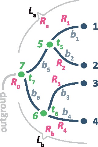
An evolutionary tree showing branch lengths (b), lineage lengths (L), lineage rates (R), and node times (t). Relative lineage rates are computed from branch lengths using equations (34)–(39) in Tamura et al. (2018). Node times and branch rates are not required for estimating relative lineage rates.
We considered the correlation between ancestral and descendant lineage rates (ρad), the correlation between the sister lineage rates (ρs), and the decay in ρad when one or two intervening branches were skipped (d1 and d2, respectively) as features (see Materials and Methods). ρad was considered as a feature because our analyses of simulated data showed that ρad was much higher for phylogenetic trees in which molecular sequences evolved under an ABR model (0.96) than an IBR model (0.54, fig. 3a). Importantly, ρad is not expected to be 0 under the IBR model because ρad is a correlation between ancestral and descendant lineages, not independent branches. An ancestral lineage includes all the lineages in the descendant subtree, therefore, the evolutionary rate of an ancestral lineage naturally depends on the evolutionary rates of its descendant lineages in RRF (Tamura et al. 2018). Therefore, ancestral and descendant lineage rates will be correlated. Although ρad is >0, it showed distinct patterns for ABR and IBR models and is, thus, a good candidate feature for McL (fig. 3a).
Fig. 3.

The relationship of (a) ancestral and direct descendant lineage rates and (b) sister lineage rates when the simulated evolutionary rates were autocorrelated with each other (red) or varied independently (blue). The correlation coefficients are shown. (c) The decay of correlation between ancestral and descendant lineages when we skip one intervening branch (d1) and when we skip two intervening branches (d2). Percent decay values are shown. (d) ROC and PR curves (inset) of CorrTest for detecting branch rate model by using only the feature of ancestor–descendant lineage rates correlation (ρad, green), only the feature of sister lineage rates correlation (ρs, orange), and all four features (all, black). The area under the curve is provided. (e) The relationship between the CorrScore produced by the McL model and the P value. IBR model can be rejected when the CorrScore is >0.83 at a significant level of P < 0.01, or when the CorrScore is >0.5 at P < 0.05.
As our second feature, we considered the correlation between the sister lineages (ρs), because ρs was higher for the ABR model (0.89) than the IBR model (0.00, fig. 3b). Two additional features considered were the decay in ρad when one or two intervening branches were skipped (d1 and d2, respectively). We expect that ρad will decay more slowly under ABR than IBR, which was confirmed (fig. 3c). The selected set of candidate features (ρs, ρad, d1, and d2) can be measured for any phylogeny with branch lengths, for example, derived from molecular data using the maximum likelihood method. They are then used to train the McL classifier (fig. 1i and j). For this purpose, we need a large set of phylogenies in which branch rates are autocorrelated for which the numerical state 1 is assigned as true positive case (fig. 1d) and phylogenies in which branch rates are independent for which the numerical state 0 is assigned as true negative case (fig. 1c).
However, there is a paucity of empirical data for which ABR and IBR are firmly established. We, therefore, trained our McL model on a simulated data set, a common practice in McL applications when reliable real world training data sets are few in number (Saminadin-Peter et al. 2012; Schrider and Kern 2016; Ekbatani et al. 2017; Le et al. 2017). We used computer simulations to generate 1,000 molecular data sets that evolved with ABR models and 1,000 molecular data sets that evolved with IBR models (fig. 1a and b). To ensure the general utility of our model for analyses of diverse data, we simulated molecular sequences with varying numbers of species, degrees of rate autocorrelation, diversity of evolutionary rates, and substitution pattern parameters (see Materials and Methods). Candidate features (ρs, ρad, d1, and d2) were computed for all 2,000 training data sets (fig. 1g and h), each of which was associated with a numerical output state (0 and 1 for IBR and ABR, respectively; fig. 1c and d). These features were used to build a predictive model by employing a logistic regression (fig. 1j). This predictive model was then used to generate a correlation score (CorrScore) for any phylogeny with branch lengths.
We also developed a conventional statistical test (CorrTest), based on CorrScore (0–1), to provide a P value to decide whether the IBR model should be rejected. A high CorrScore indicates a high probability that the branch rates are autocorrelated. At a CorrScore >0.5, Type I error (rejecting IBR when it was true) was <5%. Type I error of 1% (P value of 0.01) was achieved with a CorrScore >0.83 (fig. 3e). CorrTest is available at Github (https://github.com/cathyqqtao/CorrTest; last accessed February 6, 2019.) and in the MEGA X software (Kumar et al. 2018).
Results
We evaluated the sensitivity and specificity of our predictive model using receiver operating characteristic (ROC) curves. They measured the sensitivity of our method to detect rate autocorrelation when it was present (true positive rate, TPR) and when it was not present (false positive rate, FPR) at different CorrScore thresholds. TPR = TP/(TP +FN) and FPR = FP/(TN + FP), where TP, FN, FP, and TN stand for true positives, false negatives, false positives, and true negatives, respectively. The ROC curve for McL using all four features was the best, which led to the inclusion of all four features in the predictive model (fig. 3d; Material and Methods). The area under the ROC (AUROC) was 99%, with a 95% TPR (i.e., ABR detection) achieved at the expense of only 5% FPR (fig. 3d, black line). The area under the precision (PR) recall curve was also extremely high (0.99; fig. 3d inset), where precision and recall were defined as TP/(TP + FP) and TP/(TP + FN) (=TPR), respectively. It suggested that CorrTest detects the presence of rate autocorrelation with very high accuracy (=[TP + TN]/[TP + FP + FN + TN]) and precision.
We also performed standard cross-validation tests (fig. 1k) using the simulated data to evaluate the accuracy of the predictive model when only a subset of data are used for training. In the 10-fold cross-validation, the predictive model was developed using 90% of the simulated training data sets, and then its performance was tested on the remaining 10% of the data sets. The AUROC was >0.99 and the accuracy was high (>94%). Even in the 2-fold cross-validation, where only half of the data sets (500 ABR and 500 IBR data sets) were used for training the model, leaving the remaining half for testing, the AUROC was >0.99 and the classification accuracy was >92%. This suggested that the predictive model is robust to the size of the training set used.
We tested the performance of CorrTest on a large collection of simulated data sets where the correct rate model is known. In these data sets (Tamura et al. 2012), different software and simulation schemes were used to generate sequences with a wide range of empirically derived G + C contents, transversion/transition ratios, and evolutionary rates under both ABR and IBR models (see Materials and Methods). CorrTest accuracy was >94% in detecting ABR and IBR correctly for data sets that were simulated with low and high G + C contents (fig. 4a), small and large transition/transversion ratios (fig. 4b), and different rates of evolution (fig. 4c). As expected, CorrTest performed best on data sets that contained more and longer sequences (fig. 4d).
Fig. 4.

The performance of CorrTest in detecting ABR and IBR models in the analysis of data sets (Tamura et al. 2012) that were simulated with different (a) G + C contents, (b) transition/transversion ratios, and (c) average molecular evolutionary rates. The evolutionary rates are in the units of 10−3 substitutions per site per million years. (d–f) Patterns of CorrTest accuracy for data subsets containing 50, 100, 200, 300, and 400 ingroup sequences. The accuracy of CorrTest for different sequence lengths is shown when (d) the correct topology was assumed and (e) the topology was inferred. (f) The accuracy of CorrTest for data sets in which the inferred topology contained small and large number of topological errors. Darker color indicates higher accuracy.
In the above analyses, we used the correct tree topology and nucleotide substitution model (Hasegawa–Kishino–Yano [HKY] model (Hasegawa et al. 1985) with five discrete gamma categories). We relaxed this requirement and evaluated CorrTest by inferring the tree topology and branch lengths using the Neighbor-Joining method (Saitou and Nei 1987) with an oversimplified Kimura’s (1980) two-parameter substitution model. The estimation of the total number of substitutions between sequences was biased because inequality of nucleotide frequencies and variation of evolutionary rate across sites were not considered. Naturally, many inferred phylogenies contained topological errors, but we found the accuracy of CorrTest to be high as long as the data set contained >100 sequences of length >1,000 base pairs (fig. 4e). CorrTest also performed well even when 20% of the nontrivial tree bipartitions were incorrect in the inferred phylogeny (fig. 4f, see Materials and Methods). Therefore, CorrTest will be most reliable for large data sets and is relatively robust to errors in phylogenetic inference.
CorrTest versus Bayes Factor Analysis
We compared the performance of CorrTest with that of the Bayes factor (BF) approach. Because the BF method is computationally demanding, we limited our comparison to 100 data sets containing 100 sequences each (see Material and Methods). We computed BFs by using the stepping-stone sampling (SS) method (see Materials and Methods). BF via stepping-stone sampling (BF-SS) detected autocorrelation (P < 0.05) for 33% of the ABR data sets (fig. 5a, red curve in the ABR zone). Marginal log-likelihoods under the ABR model were very similar to or lower than those for the IBR model, which led to the failure to detect autocorrelation for 67% of ABR data sets. Therefore, BF-SS was conservative in rejecting the IBR model, as has been reported (Ho et al. 2015). CorrTest correctly detected the ABR model for 88% of the data sets (P < 0.05; fig. 5b, red curve in ABR zone). For IBR data sets, BF-SS correctly detected the IBR model for 89% (fig. 5a, blue curve in the IBR zone), whereas CorrTest correctly detected IBR model for 86% (fig. 5b, blue curve in the IBR zone). Therefore, BF-SS performs well in correctly classifying phylogenies that evolve under an IBR model, but not an ABR model. The power of CorrTest to correctly infer the ABR model is responsible for its higher overall accuracy (87% vs. 61% for BF-SS). Such a difference in accuracy was observed at different levels of statistical significance (fig. 5c) for data sets that evolved with high (v < 0.1), moderate (0.1 ≤ v < 0.2) and low (v ≥ 0.2) degree of rate autocorrelation (fig. 5d), where v is the parameter controlling the degree of rate autocorrelation (Kishino et al. 2001). However, the accuracy of CorrTest and BF-SS was similar in detecting IBR (fig. 5e). The accuracy was slightly higher for CorrTest than BF-SS for phylogenies with high (standard deviation ≥ 0.3) and low (standard deviation < 0.2) degree of independent rate variation, but the reverse was true for phylogenies with moderate (0.2 ≤ standard deviation < 0.3) degree of independent rate variation. These comparisons suggest that the McL method enables highly accurate detection of rate autocorrelation in a given phylogeny and presents an alternative to BF analyses for large data sets.
Fig. 5.

Comparisons of the performance of CorrTest and BF analyses. (a) Distributions of two times the differences of marginal log-likelihood (2 ln K) estimated under IBR and ABR models via SS method for data sets that were simulated under ABR (red) models and IBR (blue) models. ABR model is preferred (P < 0.05) when 2 ln K is >3.841 (ABR zone), and IBR model is preferred when 2lnK is <−3.841 (IBR zone). When 2 ln K is between −3.841 and 3.841, the fit of the two rate models is not significantly different (gray shade). (b) The distributions of CorrScores in analyses of ABR (red) and IBR (blue) data sets. Rates are predicted to be autocorrelated if the CorrScore is >0.5 (P < 0.05, ABR zone) and vary independently if the CorrScore is ≤0.5 (IBR zone). (c) The rate of detecting ABR model correctly (TPR) at different levels of statistical significance in Bayes factor (BF-SS) and CorrTest analyses. Posterior probabilities for ABR in BF-SS analysis are derived using the log-likelihood patterns in (a). CorrTest P values are derived using the CorrScore pattern in (b). (d) The accuracy of identifying ABR model for data sets simulated with low (v ≥ 0.2), moderate (0.1 ≤ v < 0.2), and high (v < 0.1) levels of rate autocorrelation in Kishino et al.’s (2001) model. (e) The accuracy of identifying IBR model for data sets simulated at different degrees of rate variation in Drummond et al. (2006): low (standard deviation <0.2), moderate (0.2 ≤ standard deviation < 0.3), and high (standard deviation ≥ 0.3).
Autocorrelation of Rates Is Common in Molecular Evolution
The high accuracy and fast computational speed of CorrTest enabled us to test the presence of autocorrelation in 17 large data sets from 11 published studies of eukaryotic species and 2 published studies of prokaryotic species encompassing diverse groups across the tree life. This included nuclear, mitochondrial, and plastid DNA, and protein sequences from mammals, birds, insects, metazoans, plants, fungi, parasitic protozoans, and prokaryotes (table 1). CorrTest rejected the IBR model for all data sets (P < 0.05). In these analyses, a time-reversible process was assumed for substitutions of nucleotides and amino acids in the original studies (table 1). However, the violation of this assumption may produce biased results in phylogenetic analysis (Jayaswal et al. 2014). We, therefore, applied an unrestricted substitution model (Yang 1994) for analyzing all the nucleotide data sets and found that CorrTest rejected the IBR model in every case (P < 0.05). This robustness stems from the fact that the branch lengths estimated under the time-reversible and the unrestricted model are highly correlated for these data (r2 > 0.99). This could be the reason why CorrTest produced reliable results even when an oversimplified model (Kimura 1980) was used for analyzing computer simulated data (fig. 4e and f).
Table 1.
Patterns of Rate Autocorrelation Inferred Using the CorrTest Approach.
| Taxonomic Group | Data Type | Sequence Counta | Sequence Length | Substitution Model | Rate Modelb | CorrScore | P value | 1/νc | Reference |
|---|---|---|---|---|---|---|---|---|---|
| Mammals (A) | Nuclear 4-fold degenerate sites | 138 | 1,671 | GTR + Γ | ABR & IBR | 0.98 | <0.001 | 3.21 | Meredith et al. (2011) |
| Mammals (B) | Nuclear third codon positions | 138 | 11,010 | GTR + Γ | ABR & IBR | 0.99 | <0.001 | 4.42d | Meredith et al. (2011) |
| Mammals (C) | Nuclear proteins | 138 | 11,010 | JTT + Γ | ABR & IBR | 0.99 | <0.001 | 3.11 | Meredith et al. (2011) |
| Mammals (D) | Mitochondrial DNA | 271 | 7,370 | HKY + Γ | ABR | 0.98 | <0.001 | 3.77e | Dos Reis et al. (2012) |
| Birds (A) | Nuclear DNA | 198 | 101,781 | GTR + Γ | IBR | 1.00 | <0.001 | 2.07f | Prum et al. (2015) |
| Birds (B) | Nuclear third codon positions | 222 | 1,364 | GTR + Γ | IBR | 1.00 | <0.001 | 2.11 | Claramunt and Cracraft (2015) |
| Birds (C) | Nuclear first and second codon positions | 222 | 2,728 | GTR + Γ | IBR | 1.00 | <0.001 | 2.53 | Claramunt and Cracraft (2015) |
| Insects | Nuclear proteins | 143 | 220,091 | LG + Γ | IBR | 1.00 | <0.001 | 8.68g | Misof et al. (2014) |
| Metazoans | Mitochondrial and nuclear proteins | 113 | 2,049 | LG + Γ | ABR | 0.65 | <0.05 | 40.00 | Erwin et al. (2011) |
| Plants (A) | Plastid third codon positions | 335 | 19,449 | GTR + Γ | NA | 1.00 | <0.001 | 2.28 | Ruhfel et al. (2014) |
| Plants (B) | Plastid proteins | 335 | 19,449 | JTT + Γ | NA | 1.00 | <0.001 | 2.46 | Ruhfel et al. (2014) |
| Plants (C) | Nuclear first and second codon positions | 99 | 290,718 | GTR + Γ | NA | 1.00 | <0.001 | 5.50 | Wickett et al. (2014) |
| Plants (D) | Chloroplast and nuclear DNA | 124 | 5,992 | GTR + Γ | IBR | 1.00 | <0.001 | 2.64 | Beaulieu et al. (2015) |
| Fungi | Nuclear proteins | 85 | 609,772 | LG + Γ | NA | 0.97 | <0.001 | 3.78 | Shen et al. (2016) |
| Parasitic protozoans | Mitochondrial DNA | 91 | 6,863 | HKY + Γ | ABR & IBR | 0.87 | <0.01 | 2.41 | Pacheco et al. (2018) |
| Prokaryotes (A) | Nuclear proteins | 197 | 6,884 | JTT + Γ | ABR | 0.79 | <0.05 | 2.54 | Battistuzzi and Hedges (2009) |
| Prokaryotes (B) | Nuclear proteins | 126 | 3,145 | JTT + Γ | NA | 0.83 | <0.05 | 1.23 | Calteau et al. (2014) |
Counts exclude outgroup taxa.
The branch rate model used in the original study. ABR, autocorrelated branch rate model; IBR, independent branch rate model; NA, no rate model information available.
1/ν is the inverse of the autocorrelation parameter that is estimated by MCMCTree using the ABR model in the time unit of 100 My.
1/v were 2.13 and 2.09 for each subtree in mammals (B).
1/v were 3.73, 1.04, and 2.47 for each subtree in mammals (D).
1/v were 1.60 and 2.07 for each subtree in birds (A).
1/v were 17.24 and 9.62 for each subtree in insects.
These results suggest that the autocorrelation of rates among lineages is very common in molecular phylogenies. This pattern contrasts starkly with those reported in many previous studies (Drummond et al. 2006; Moore and Donoghue 2007; Brown et al. 2008; Bell et al. 2010; Smith et al. 2010; Linder et al. 2011; Jarvis et al. 2014; Lu et al. 2014; Barreda et al. 2015; Claramunt and Cracraft 2015; Prum et al. 2015; Feng et al. 2017; Barba-Montoya et al. 2018). In fact, all but three data sets (Battistuzzi and Hedges 2009; Erwin et al. 2011; Calteau et al. 2014) received very high CorrScores, resulting in extremely significant P values (P < 0.01). The IBR model was also rejected for the three data sets (P < 0.05), but their CorrScores were not as high, likely because of limited or biased sampling of the evolutionary diversity. For example, the metazoan data set (Erwin et al. 2011) contains sequences primarily from highly divergent species that share common ancestors hundreds of millions of years ago. In this case, tip branches in the phylogeny are long and their evolutionary rates are influenced by many unsampled lineages. Such sampling effects weaken the rate autocorrelation signal. We verified this behavior via an analysis of simulated data and found that CorrScores decreased when density of taxon sampling was lower (fig. 6). Overall, CorrTest detected rate autocorrelation in all the empirical data sets.
Fig. 6.
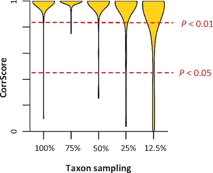
The distribution of CorrScore for data sets (Tamura et al. 2012) with different taxon sampling densities. The CorrScore decreases when the density of taxon sampling is lower, as there is much less information to discriminate between ABR and IBR models. Red dashed lines mark two statistical significance levels of 5% and 1%. Results are summarized from 100 simulated data sets for each taxon sampling category.
Magnitude of Rate Autocorrelation in Molecular Data
CorrScore is influenced by the size of the data set in addition to the degree of autocorrelation, so it is not a direct measure of the degree of rate autocorrelation (effect size) in a phylogeny. Instead, one should use a Bayesian approach to estimate the degree of rate autocorrelation, for example, under Kishino et al.’s (2001) autocorrelated rate model. In this model, a single parameter (ν) captures the degree of autocorrelation among branches in a phylogenetic tree. A low value of ν indicates high autocorrelation, so, we use the inverse of v to represent the degree of rate autocorrelation. MCMCTree (Yang 2007) analyses of 100 simulated data sets (see Materials and Methods) confirmed that the estimated v was related linearly with the true value (fig. 7). Based on the results from the analysis of empirical data sets, we suggest that 1/v > 3 be considered high autocorrelation, 1/v between 1 and 3 be considered moderate autocorrelation, and 1/v below 1 be considered weak autocorrelation. Based on this ad hoc criterion, we may conclude that rate autocorrelation is moderate to high for empirical data sets examined for species across the tree of life.
Fig. 7.
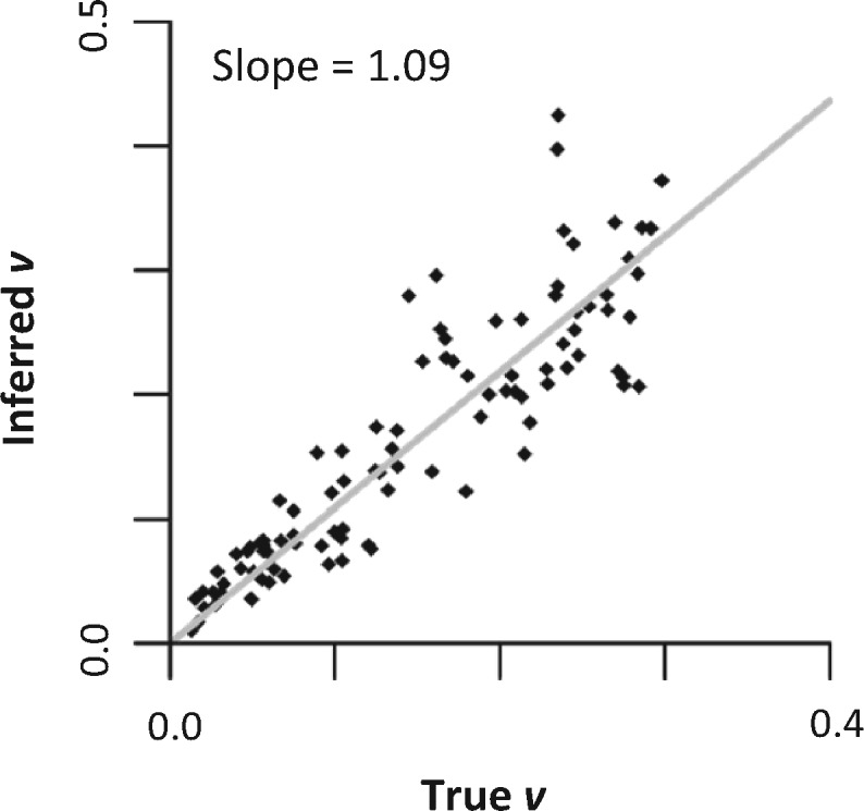
The relationship between the inferred autocorrelation parameter (v) from MCMCTree and the true value for data sets simulated under ABR models with the true v ranging from 0.01 to 0.3. The gray line represents the best-fit regression line, which has a slope of 1.09.
Other interesting patterns emerge from this analysis. First, rate autocorrelation is highly significant for mutational rates (=substitution rate at neutral positions), which are expected to be similar in sister species because they inherit cellular machinery from a common ancestor (table 1). The substitution rates at the third codon positions and the 4-fold degenerate sites are considered to be a good proxy of synonymous substitution rate, because they are largely neutral and are the best reflection of mutation rates (Kumar and Subramanian 2002). For example, the mammalian data sets A and B, which consisted of the 4-fold degenerate sites and the third codon positions, received high CorrScores of 0.99 and 0.98, respectively (P < 0.001). Second, our model detected a strong signal of autocorrelation among amino acid substitution rates, which were dictated by natural selection (table 1). For example, mammalian data set C received a high CorrScore of 0.99 in the proteins encoded in the same genes in the data sets of third codon positions (mammalian data set B) and 4-fold degenerate sites (mammalian data set A). Bayesian analyses also showed that the degree of rate autocorrelation is similar: inverse of v was 3.21 in 4-fold degenerate sites and 3.11 in amino acid sequences for mammalian data sets. Third, mutational and substitution rates in nuclear genomes and substitution rates in mitochondrial genomes are highly autocorrelated (P < 0.05, table 1) (synonymous substitution rate was not used for mitochondrial data). These results establish that molecular and nonmolecular evolutionary patterns are concordant, because morphological characteristics are correlated with taxonomic or geographic distance (Wyles et al. 1983; Sargis and Dagosto 2008; Lanfear et al. 2010; Cox and Hautier 2015; Shao et al. 2016).
Discussion
Our results demonstrate that a McL framework is useful to develop a method to detect the presence of rate autocorrelation among branches in a phylogeny. This method yields CorrScore estimates that enables development of a conventional statistical test (CorrTest) to detect autocorrelation. This method can be used for data sets with small (50–100) and large numbers of sequences, as supported by high accuracy achieved by CorrTest in the analysis of simulated data sets (fig. 4). We also evaluated if higher accuracy could be achieved by building specific predictive models that were trained separately using data with different ranges of the number of sequences (n): M100 (n ≤ 100), M200 (100 < n ≤ 200), M300 (200 < n ≤ 300), and M400 (n > 300). A specific threshold for CorrScore that corresponded to certain P value was determined for each training subset and then tested using Tamura et al.’s (2012) simulated data with the corresponding number of sequences. For example, we used the threshold determined for the model trained with small data (M100) on the test data that contained ≤100 sequences, and used the threshold determined for the model trained with large data (M400) on the large test data (400 sequences). We found that the accuracy obtained by using the specific thresholds determined for data sets with different numbers of sequences (M100–M400) (fig. 8) was similar to the accuracy obtained by using a global threshold (fig. 4d–f). This is because the McL algorithm automatically incorporated the impact of the number of sequences when determining the relationship of four selected features (ρs, ρad, d1, and d2). This justifies the usage of the globally trained CorrTest that we used in all the empirical analyses reported here.
Fig. 8.

Patterns of CorrTest accuracy using the specific thresholds determined by predictive models trained with different ranges of the number of sequences (n): M100 (n ≤ 100), M200 (100 < n ≤ 200), M300 (200 < n ≤ 300), and M400 (n > 300) for the corresponding test data sets (Tamura et al. 2012). Accuracies are shown for 50, 100, 200, 300, and 400 ingroup sequences. The accuracy of CorrTest for different sequence lengths is shown when (a) the correct topology was assumed and (b) the topology was inferred. (c) The accuracy of CorrTest for data sets in which the inferred topology contained small and large number of topological errors. Darker color indicates higher accuracy.
No single branch rate model may be adequate for Bayesian dating analyses, and one may need to use a mixture of models because different groups of species and genes in a large phylogeny may have evolved with different levels of autocorrelation (e.g., Lartillot et al. 2016; Tamura et al. 2018). In this sense, results produced by CorrTest (and by BF) analyses primarily detect the presence of rate autocorrelation, but they do not tell us if the rate autocorrelation exists in every clade of a phylogeny or if the degree of autocorrelation is the same in all the clades. One may apply CorrTest to individual clades (subtrees) to evaluate these patterns. For example, we divided a few large empirical phylogenies (Meredith et al. 2011; Dos Reis et al. 2012; Misof et al. 2014; Prum et al. 2015) into subtrees with at least 50 sequences and applied CorrTest on subtrees to detect the existence of clade-specific rate autocorrelation. These analyses showed a wide range of 1/v values, which was consistent with the large range of the autocorrelation parameter values observed for different data sets we analyzed (1.2 < 1/v < 40, table 1). That is, the degree of autocorrelation likely varies among different types of genes, different types of substitutions, and in different taxonomic groups. In the future, it will be useful to identify such patterns at micro- and macro-evolutionary scales and to elucidate mechanistic underpinnings of the differences observed.
Conclusion
We have presented a fast, scalable, and accurate method (CorrTest) to detect the presence of branch rate autocorrelation in a phylogeny. In addition to molecular data, CorrTest may be used for testing autocorrelation of rates in nonmolecular data, for example, morphological characteristics, because the features required for CorrTest can be calculated for any phylogeny with branch lengths. The application of CorrTest to a large number of data sets addressed an enduring question in evolutionary biology: Are the molecular rates of change between species correlated or independent? We find that the rate autocorrelation is the rule, rather than the exception. So, it will be best to employ an ABR model in molecular dating analyses in studies of biodiversity, phylogeography, development, and genome evolution. However, when in doubt, one may conduct CorrTest, which is particularly effective for analyzing large data sets. We also expect CorrTest to be useful in analyzing many other large data sets, revealing both the extent of autocorrelated evolutionary rates in the tree of life and the exceptions to this rule. Discovery of genes, gene families, and species groups in which branch rates are evolving without significant autocorrelation will be precursors to elucidating mechanistic underpinnings of new biological phenomena.
Materials and Methods
McL Model
Training Data for McL
We simulated nucleotide alignments using IBR and ABR models using the NELSI package (Ho et al. 2015) with a variety of empirically derived parameter values and parameters used in previous studies (Rosenberg and Kumar 2003; Ho et al. 2015). In IBR cases, branch-specific rates were drawn from a lognormal distribution with a mean gene-by-gene substitution rate and a standard deviation (in log-scale) that varied from 0.1 to 0.4, previously used in a study simulating independent rates with different levels of variation (Ho et al. 2015). In ABR cases, branch-specific rates were simulated under an autocorrelated process (Kishino et al. 2001), using equation (10.9) in Yang (2014). The initial rate was set as the mean rate derived from an empirical gene and an autocorrelated parameter, ν, that was randomly chosen from a uniform distribution ranging from 0.01 to 0.3, following a previous simulation of low, moderate and high degree of rate autocorrelation (Ho et al. 2015). We used SeqGen (Grassly et al. 1997) to generate alignments under the HKY model (Hasegawa et al. 1985) with four discrete gamma categories. This process used a master phylogeny, consisting of 60–400 ingroup taxa randomly sampled from the bony-vertebrate clade in the TimeTree of Life (Hedges and Kumar 2009). Mean evolutionary rates, G + C contents, transition/transversion ratios and numbers of sites for simulation were derived from empirical distributions (Rosenberg and Kumar 2003). One thousand molecular data sets were generated under ABR and IBR models separately and these 2,000 simulated data sets were used as training data in building the McL model.
Calculation of Features for McL
Lineage-specific rate estimates (Ri’s) were obtained using equations (28)–(31) and (34)–(39) in Tamura et al. (2018). For any given node in the phylogeny (e.g., node 5 in fig. 2), we extracted the relative rates of its ancestral lineage (e.g., Ra in fig. 2) and two direct descendant lineages (e.g., R1 and R2 in fig. 2). Then, we calculated correlation between the ancestral lineage and its direct descendant lineage rate to obtain estimates of ancestor–descendant rate correlation (ρad). We also calculated correlation between sister lineage rates (ρs). We need to assign labels to lineage rates of each sister pair to determine which lineage is the first sister lineage and which lineage is the second sister lineage, for example, (R1 and R2) or (R2 and R1) in fig. 2. If rates of the first sister lineages are always higher than rates of the second sister lineages, an artificial correlation will be generated between sister lineage rates. To avoid this possibility, we randomly labeled sister lineages. The labeling of sister pairs have negligible impact (<2%) on ρs when the number of sequences in the phylogeny is not too small (>50). For smaller data sets, we found that it is best to generate multiple ρs estimates, each using randomly labeled sister pairs, to eliminate bias that may result from the arbitrary designation of sister pairs. In this case, we recommend using the mean ρs from multiple replicates in the CorrTest analysis. To avoid the assumption of linear correlation between lineages, we used Spearman rank correlation because it can detect both linear and nonlinear correlation between two vectors. Two additional features were included in McL model: d1 and d2, which are the decay of ρad when one or two intervening branches are skipped. We first estimated ρad_skip1 as the correlation between rates where the ancestor and descendant were separated by one intervening branch, and ρad_skip2 as the correlation between rates where the ancestor and descendant were separated by two intervening branches. This skipping reduces ancestor–descendant correlation, which we then used to derive the decay of correlation values by using equations d1 = (ρad − ρad_skip1)/ρad and d2 = (ρad − ρad_skip2)/ρad. These two features improved the accuracy of our model slightly. In the analysis of empirical data sets, we found that a large amount of missing data (>50%) can result in unreliable estimates of branch lengths and other phylogenetic errors (Wiens and Moen 2008; Lemmon et al. 2009; Filipski et al. 2014; Xi et al. 2016; Marin and Hedges 2018). In this case, we recommend computing selected features (ρs, ρad, d1, and d2) using only those lineage pairs for which >50% of the positions contain valid data, or removing sequences with a large amount of missing data.
Building the McL Predictive Model
We trained a predictive model with only ρad, only ρs or all four features (ρs, ρad, d1, and d2) using 2,000 simulated training data sets (1,000 with ABR model and 1,000 with IBR model). For each set of training data, we inferred the branch lengths from the molecular sequences with a fixed topology first and used these inferred branch lengths to estimate relative lineage rates for computing selected features. A numerical state of 1 was given to true positive cases (autocorrelated rates) and 0 was assigned to true negative cases (independent rates). Then, a predictive model was generated via logistic regression in the skit-learn model (Pedregosa et al. 2011), which is a python toolbox for data mining and data analysis using McL algorithms. This model contains the relationship between the numerical state and the selected features. Therefore, for any phylogeny with branch lengths, we can calculate features and apply the predictive model to generate a numerical output value between 0 and 1. The resulting value is referred as the CorrScore. A high CorrScore suggests that the rates are more likely to be autocorrelated. Every CorrScore associates with a Type I error (P value), which is the percentage of IBR cases that are incorrectly predicted as ABR. We found that Type I error of 5% (P value of 0.05) was achieved with a CorrScore >0.5, and Type I error of 1% was achieved with a CorrScore >0.83. Therefore, we developed a conventional statistical test (CorrTest) based on CorrScore. CorrScores of 0.5 and 0.83 were used as the global thresholds at 5% and 1% significant levels. Using the same procedure, we also trained specific predictive models using training data with different numbers of sequences (n): M100 (n ≤ 100), M200 (100 < n ≤ 200), M300 (200 < n ≤ 300), and M400 (n > 300) and determined specific threshold for CorrScore for each model. CorrScores of 0.69, 0.61, 0.57, and 0.31 were thresholds for M100, M200, M300, and M400 at 5% significant level, respectively. CorrScores of 0.84, 0.86, 0.88, and 0.73 were thresholds for M100, M200, M300, and M400 at 1% significant level, respectively.
Test Data Sets
Tamura et al.’s (2012) simulated data sets were used to evaluate CorrTest’s performance. This allowed us to test the performance of our method on ABR and IBR data sets with different G + C contents (range 39–82%), transition/transversion ratios (range 1.9–6.0), and evolutionary rates (range 1.35–2.60 substitution per site per billion years). In IBR simulations, Tamura et al. (2012) used a uniform distribution in which branch rates were sampled from a uniform density in the interval [(1 − x).r – (1 + x).r], where r is the mean evolutionary rate and the x is the degree of rate variation (0.5 or 1.0 for 50% and 100% rate variation). For ABR simulations, Tamura et al. (2012) used Kishino et al.’s (2001) model with ν = 1. In both scenarios, sequences were simulated on a master phylogeny of 400 ingroup taxa using the HKY substitution model with 5 discrete gamma categories. We analyzed 100 data sets simulated using the ABR model and 100 data sets simulated using the IBR model (50% rate variation). We also randomly sampled 50, 100, 200, and 300 sequences from the full set of 400 ingroup sequences, and conducted CorrTest using the correct topology and error-prone topology inferred by the Neighbor-Joining method (Saitou and Nei 1987) with an oversimplified substitution model of Kimura (1980) with both global and specific CorrScore thresholds. The percentage of incorrect inferred tree bipartitions (clades) was calculated by d/[2(m − 3)] where d was the Robinson and Foulds’s (1981) topological distance between inferred and true topologies and m was the number of sequences. In addition, we also tested CorrTest’s performance on 100 data sets simulated by Tamura et al. (2012) under an IBR model with 100% rate variation. CorrTest worked perfectly (100% accuracy) for these data sets (results not shown).
In addition to above analyses, we conducted another set of simulations to generate 100 data sets using IBR (independent lognormal distribution) and ABR (autocorrelated lognormal distribution) (Kishino et al. 2001) models, each using the same strategy as in training data simulation (described above) on a master phylogeny of 100 taxa randomly sampled from the bony-vertebrate clade in the TimeTree of Life (Hedges and Kumar 2009). These 200 data sets were used to conduct CorrTest and BF analyses and to obtain the autocorrelation parameter (v) in MCMCTree (Yang 2007).
CorrTest Analyses
All CorrTest analyses were conducted using customized R code (available at https://github.com/cathyqqtao/CorrTest, last accessed February 6, 2019). We first estimated branch lengths of a phylogeny for sequence alignments using the maximum likelihood method with the correct substitution model and the correct topology in MEGA 7 command line version (Kumar et al. 2012; Kumar et al. 2016). We used Neighbor-Joining method to estimate topology and branch lengths with Kimura’s (1980) two-parameter substitution model and without the assumption of rate variation across sites under the gamma distribution in MEGA 7 command line version, when we tested the robustness of our model to topological error. We then used the estimated branch lengths to compute relative lineage rates using RRF (Tamura et al. 2012, 2018) and calculated the value of selected features (ρs, ρad, d1, and d2) to obtain the CorrScore. We conducted CorrTest on the CorrScore to estimate the P value of detecting rate autocorrealtion. No calibration was needed for CorrTest analyses. CorrTest is also available in the MEGA X software (Kumar et al. 2018).
BF Analyses
We computed the BF-SS (Xie et al. 2011) with n = 20 and a = 5 using mcmc3r (Dos Reis et al. 2018). BF-SS estimates the marginal likelihoods using the idea from importance sampling, a common practice in statistics, to construct a path between prior and posterior distributions of a model (Xie et al. 2011; Baele et al. 2013). We chose BF-SS because the harmonic mean estimator has many statistical shortcomings (Lepage et al. 2007; Xie et al. 2011; Baele et al. 2013) and thermodynamic integration (Lartillot and Philippe 2006) is less efficient than BF-SS (Baele et al. 2012). For each data set, we computed the log-likelihoods (ln K) under the IBR and ABR models. The BF posterior probability for ABR was calculated as shown in Dos Reis et al. (2018). We used only one calibration point at the root (true age with a narrow uniform distribution) in all the Bayesian analyses, as it is the minimum number of calibrations required by MCMCTree (Yang 2007). For other priors, we used diffused distributions of “rgene_gamma = 1 1,” “sigma2_gamma = 1 1,” and “BDparas = 1 1 0.” In all Bayesian analyses, two independent runs of 5,000,000 generations each were conducted, and results were checked in Tracer (Rambaut et al. 2018) for convergence. ESS values were higher than 200 after removing 10% burn-in samples for each run.
Analysis of Empirical Data Sets
We used 17 data sets from 11 published studies of eukaryotes and 2 published studies of prokaryotes that cover the major groups in the tree of life (table 1). These data were selected for relative completeness (missing data <50%) and large sample size (>80 sequences). As we know, a large amount of missing data (>50%) can result in unreliable estimates of branch lengths and other phylogenetic errors (Wiens and Moen 2008; Lemmon et al. 2009; Filipski et al. 2014; Xi et al. 2016; Marin and Hedges 2018) and potentially bias CorrTest results. When a phylogeny with branch lengths was available from the original study, we estimated relative rates directly from the branch lengths via RRF (Tamura et al. 2018) and computed selected features (ρs, ρad, d1, and d2) to conduct CorrTest. Otherwise, maximum likelihood estimates of branch lengths were obtained in MEGA 7 command line version (Kumar et al. 2012; Kumar et al. 2016) using the published topology, sequence alignments, and the substitution model specified in the original article. To examine the impact of the specification of a time-reversible substitution model on CorrTest, we estimated branch lengths under an unrestricted substitution model (Yang 1994) for all the nucleotide data sets in PAML (Yang 2007) and conducted CorrTest.
To obtain the autocorrelation parameter (v), we used MCMCTree (Yang 2007) with the same input priors as the original study, but omitting calibration priors to avoid the influence of calibration uncertainty densities on the estimate of v. We did, however, provide a root calibration because MCMCTree required it. For this purpose, we specified the root calibration as the one used in the original article or as the median age of the root node in the TimeTree database (Hedges et al. 2006; Kumar et al. 2017) ±50 My (uniform distribution with 2.5% relaxation on minimum and maximum bounds). Bayesian analyses required long computational times, so we used the original alignments in MCMCTree to infer v if alignments were shorter than 20,000 sites. If the alignments were longer than 20,000 sites, we randomly selected 20,000 sites from the original alignments. However, one data set (Ruhfel et al. 2014) contained more than 300 ingroup species, such that even alignments of 20,000 sites required prohibitive amounts of memory. In this case, we randomly selected 2,000 sites from the original alignments to use in MCMCTree for v inference (similar results were obtained with a different site subset). Two independent runs were conducted for each data set, and results were checked in Tracer (Rambaut et al. 2018) for convergence. ESS values were higher than 200 after removing 10% burn-in samples for each run. All empirical data sets are available at https://github.com/cathyqqtao/CorrTest (last accessed February 6, 2019).
Acknowledgments
We thank Xi Hang Cao for assisting on building the McL model, and Drs Bui Quang Minh, Beatriz Mello, Heather Rowe, Ananias Escalante, Maria Pacheco, Jose Barba-Montoya, Antonia Chroni, and S. Blair Hedges for critical comments and editorial suggestions. This research was supported by grants from National Aeronautics and Space Administration (NASA NNX16AJ30G), National Institutes of Health (GM0126567-01 and LM012487-03), National Science Foundation (NSF 1661218), Pennsylvania Department of Health (TU-420721) and Tokyo Metropolitan University (DB105).
References
- Baele G, Lemey P, Bedford T, Rambaut A, Suchard MA, Alekseyenko AV.. 2012. Improving the accuracy of demographic and molecular clock model comparison while accommodating phylogenetic uncertainty. Mol Biol Evol. 29(9): 2157–2167. [DOI] [PMC free article] [PubMed] [Google Scholar]
- Baele G, Lemey P, Vansteelandt S.. 2013. Make the most of your samples: Bayes factor estimators for high-dimensional models of sequence evolution. BMC Bioinformatics 14:85.. [DOI] [PMC free article] [PubMed] [Google Scholar]
- Baele G, Li WLS, Drummond AJ, Suchard MA, Lemey P.. 2013. Accurate model selection of relaxed molecular clocks in Bayesian phylogenetics. Mol Biol Evol. 30(2): 239–243. [DOI] [PMC free article] [PubMed] [Google Scholar]
- Barba-Montoya J, Dos Reis M, Schneider H, Donoghue PCJ, Yang Z.. 2018. Constraining uncertainty in the timescale of angiosperm evolution and the veracity of a Cretaceous Terrestrial Revolution. New Phytol. 218(2): 819–834. [DOI] [PMC free article] [PubMed] [Google Scholar]
- Barreda VD, Palazzesi L, Tellería MC, Olivero EB, Raine JI, Forest F.. 2015. Early evolution of the angiosperm clade Asteraceae in the Cretaceous of Antarctica. Proc Natl Acad Sci U S A. 112(35): 10989–10994. [DOI] [PMC free article] [PubMed] [Google Scholar]
- Battistuzzi FU, Filipski A, Hedges SB, Kumar S.. 2010. Performance of relaxed-clock methods in estimating evolutionary divergence times and their credibility intervals. Mol Biol Evol. 27(6): 1289–1300. [DOI] [PMC free article] [PubMed] [Google Scholar]
- Battistuzzi FU, Hedges SB.. 2009. A major clade of prokaryotes with ancient adaptations to life on land. Mol Biol Evol. 26(2): 335–343. [DOI] [PubMed] [Google Scholar]
- Beaulieu JM, O’Meara BC, Crane P, Donoghue MJ.. 2015. Heterogeneous rates of molecular evolution and diversification could explain the Triassic age estimate for angiosperms. Syst Biol. 64(5): 869–878. [DOI] [PubMed] [Google Scholar]
- Bell CD, Soltis DE, Soltis PS.. 2010. The age and diversification of the angiosperms re-revisited. Am J Bot. 97(8): 1296–1303. [DOI] [PubMed] [Google Scholar]
- Brown JW, Rest JS, García-Moreno J, Sorenson MD, Mindell DP.. 2008. Strong mitochondrial DNA support for a Cretaceous origin of modern avian lineages. BMC Biol. 6:6.. [DOI] [PMC free article] [PubMed] [Google Scholar]
- Buck CB, Van Doorslaer K, Peretti A, Geoghegan EM, Tisza MJ, An P, Katz JP, Pipas JM, McBride AA, Camus AC, et al. 2016. The ancient evolutionary history of polyomaviruses. PLoS Pathog. 12(4): e1005574.. [DOI] [PMC free article] [PubMed] [Google Scholar]
- Bzdok D, Krzywinski M, Altman N.. 2018. Machine learning: supervised methods. Nat Methods. 15(1): 5–6. [DOI] [PMC free article] [PubMed] [Google Scholar]
- Calteau A, Fewer DP, Latifi A, Coursin T, Laurent T, Jokela J, Kerfeld CA, Sivonen K, Piel J, Gugger M.. 2014. Phylum-wide comparative genomics unravel the diversity of secondary metabolism in Cyanobacteria. BMC Genomics. 15:977.. [DOI] [PMC free article] [PubMed] [Google Scholar]
- Christin P-A, Spriggs E, Osborne CP, Strömberg CAE, Salamin N, Edwards EJ.. 2014. Molecular dating, evolutionary rates, and the age of the grasses. Syst Biol. 63(2): 153–165. [DOI] [PubMed] [Google Scholar]
- Christin S, Hervet E, Lecomte N.. 2018. Applications for deep learning in ecology. bioRxiv doi: 10.1101/334854 (last accessed February 6, 2019). [DOI]
- Claramunt S, Cracraft J.. 2015. A new time tree reveals Earth history’s imprint on the evolution of modern birds. Sci Adv. 1(11): e1501005.. [DOI] [PMC free article] [PubMed] [Google Scholar]
- Cox PG, Hautier L, editors. 2015. Evolution of the rodents: volume 5: advances in phylogeny, functional morphology and development. Cambridge: Cambridge University Press. [Google Scholar]
- Dos Reis M, Donoghue PC, Yang Z.. 2016. Bayesian molecular clock dating of species divergences in the genomics era. Nat Rev Genet. 17(2): 71–80. [DOI] [PubMed] [Google Scholar]
- Dos Reis M, Gunnell GF, Barba-Montoya J, Wilkins A, Yang Z, Yoder AD.. 2018. Using phylogenomic data to explore the effects of relaxed clocks and calibration strategies on divergence time estimation: primates as a test case. Syst Biol. 67(4): 594–615. [DOI] [PMC free article] [PubMed] [Google Scholar]
- Dos Reis M, Inoue J, Hasegawa M, Asher RJ, Donoghue PC, Yang Z.. 2012. Phylogenomic datasets provide both precision and accuracy in estimating the timescale of placental mammal phylogeny. Proc R Soc B 279(1742): 3491–3500. [DOI] [PMC free article] [PubMed] [Google Scholar]
- Dos Reis M, Thawornwattana Y, Angelis K, Telford MJ, Donoghue PC, Yang Z.. 2015. Uncertainty in the timing of origin of animals and the limits of precision in molecular timescales. Curr Biol. 25:1–12. [DOI] [PMC free article] [PubMed] [Google Scholar]
- Dos Reis M, Zhu T, Yang Z.. 2014. The impact of the rate prior on Bayesian estimation of divergence times with multiple loci. Syst Biol. 64:555–565. [DOI] [PMC free article] [PubMed] [Google Scholar]
- Drummond AJ, Ho SYW, Phillips MJ, Rambaut A.. 2006. Relaxed phylogenetics and dating with confidence. PLoS Biol. 4:88–99. [DOI] [PMC free article] [PubMed] [Google Scholar]
- Ekbatani HK, Pujol O, Segui S.. 2017. Synthetic data generation for deep learning in counting pedestrians In: Proceedings of the 6th International Conference on Pattern Recognition Applications and Methods (ICPRAM). p. 318–323. Porto, Portugal. [Google Scholar]
- Erwin DH, Laflamme M, Tweedt SM, Sperling EA, Pisani D, Peterson KJ.. 2011. The Cambrian conundrum: early divergence and later ecological success in the early history of animals. Science 334(6059): 1091–1097. [DOI] [PubMed] [Google Scholar]
- Feng Y-J, Blackburn DC, Liang D, Hillis DM, Wake DB, Cannatella DC, Zhang P.. 2017. Phylogenomics reveals rapid, simultaneous diversification of three major clades of Gondwanan frogs at the Cretaceous–Paleogene boundary. Proc Natl Acad Sci U S A. 114(29): E5864–E5870. [DOI] [PMC free article] [PubMed] [Google Scholar]
- Filipski A, Murillo O, Freydenzon A, Tamura K, Kumar S.. 2014. Prospects for building large timetrees using molecular data with incomplete gene coverage among species. Mol Biol Evol. 31(9): 2542–2550. [DOI] [PMC free article] [PubMed] [Google Scholar]
- Foster CS, Sauquet H, Van der Merwe M, McPherson H, Rossetto M, Ho SY.. 2016. Evaluating the impact of genomic data and priors on Bayesian estimates of the angiosperm evolutionary timescale. Syst Biol. 66:338–351. [DOI] [PubMed] [Google Scholar]
- Gillespie JH. 1984. The molecular clock may be an episodic clock. Proc Natl Acad Sci U S A. 81(24): 8009–8013. [DOI] [PMC free article] [PubMed] [Google Scholar]
- Grassly NC, Adachi J, Rambaut A.. 1997. Seq-Gen: an application for the Monte Carlo simulation of protein sequence evolution along phylogenetic trees. Comput Appl Biosci. 13:235–238. [DOI] [PubMed] [Google Scholar]
- Hasegawa M, Kishino H, Yano T.. 1985. Dating of the human-ape splitting by a molecular clock of mitochondrial DNA. J Mol Evol. 22(2): 160–174. [DOI] [PubMed] [Google Scholar]
- Hedges SB, Dudley J, Kumar S.. 2006. TimeTree: a public knowledge-base of divergence times among organisms. Bioinformatics 22(23): 2971–2972. [DOI] [PubMed] [Google Scholar]
- Hedges SB, Kumar S.. 2009. The TimeTree of life. New York: Oxford University Press. [Google Scholar]
- Hertweck KL, Kinney MS, Stuart SA, Maurin O, Mathews S, Chase MW, Gandolfo MA, Pires JC.. 2015. Phylogenetics, divergence times and diversification from three genomic partitions in monocots. Bot J Linn Soc. 178(3): 375–393. [Google Scholar]
- Ho SY, Duchêne S.. 2014. Molecular-clock methods for estimating evolutionary rates and timescales. Mol Ecol. 23(24): 5947–5965. [DOI] [PubMed] [Google Scholar]
- Ho SY, Duchêne S, Duchêne D.. 2015. Simulating and detecting autocorrelation of molecular evolutionary rates among lineages. Mol Ecol Resour. 15(4): 688–696. [DOI] [PubMed] [Google Scholar]
- Jarvis ED, Mirarab S, Aberer AJ, Li B, Houde P, Li C, Ho SYW, Faircloth BC, Nabholz B, Howard JT, et al. 2014. Whole-genome analyses resolve early branches in the tree of life of modern birds. Science 346(6215): 1320–1331. [DOI] [PMC free article] [PubMed] [Google Scholar]
- Jayaswal V, Wong TK, Robinson J, Poladian L, Jermiin LS.. 2014. Mixture models of nucleotide sequence evolution that account for heterogeneity in the substitution process across sites and across lineages. Syst Biol. 63(5): 726–742. [DOI] [PubMed] [Google Scholar]
- Kimura M. 1980. A simple method for estimating evolutionary rates of base substitutions through comparative studies of nucleotide sequences. J Mol Evol. 16(2): 111–120. [DOI] [PubMed] [Google Scholar]
- Kimura M. 1983. The neutral theory of molecular evolution. Cambridge: Cambridge University Press. [Google Scholar]
- Kishino H, Thorne JL, Bruno WJ.. 2001. Performance of a divergence time estimation method under a probabilistic model of rate evolution. Mol Biol Evol. 18(3): 352–361. [DOI] [PubMed] [Google Scholar]
- Kumar S. 2005. Molecular clocks: four decades of evolution. Nat Rev Genet. 6(8): 654–662. [DOI] [PubMed] [Google Scholar]
- Kumar S, Hedges SB.. 2016. Advances in time estimation methods for molecular data. Mol Biol Evol. 33(4): 863–869. [DOI] [PMC free article] [PubMed] [Google Scholar]
- Kumar S, Stecher G, Li M, Knyaz C, Tamura K.. 2018. MEGA X: Molecular Evolutionary Genetics Analysis across computing platforms. Mol Biol Evol. 35(6): 1547–1549. [DOI] [PMC free article] [PubMed] [Google Scholar]
- Kumar S, Stecher G, Peterson D, Tamura K.. 2012. MEGA-CC: Computing Core of Molecular Evolutionary Genetics Analysis program for automated and iterative data analysis. Bioinformatics 28(20): 2685–2686. [DOI] [PMC free article] [PubMed] [Google Scholar]
- Kumar S, Stecher G, Suleski M, Hedges SB.. 2017. TimeTree: a resource for timelines, timetrees, and divergence times. Mol Biol Evol. 34(7): 1812–1819. [DOI] [PubMed] [Google Scholar]
- Kumar S, Stecher G, Tamura K.. 2016. MEGA7: Molecular Evolutionary Genetics Analysis version 7.0 for bigger datasets. Mol Biol Evol. 33(7): 1870–1874. [DOI] [PMC free article] [PubMed] [Google Scholar]
- Kumar S, Subramanian S.. 2002. Mutation rates in mammalian genomes. Proc Natl Acad Sci U S A. 99(2): 803–808. [DOI] [PMC free article] [PubMed] [Google Scholar]
- Lanfear R, Welch JJ, Bromham L.. 2010. Watching the clock: studying variation in rates of molecular evolution between species. Trends Ecol Evol. 25(9): 495–503. [DOI] [PubMed] [Google Scholar]
- Lartillot N, Philippe H.. 2006. Computing Bayes factors using thermodynamic integration. Syst Biol. 55(2): 195–207. [DOI] [PubMed] [Google Scholar]
- Lartillot N, Phillips MJ, Ronquist F.. 2016. A mixed relaxed clock model. Philos Trans R Soc B 371(1699): 20150132.. [DOI] [PMC free article] [PubMed] [Google Scholar]
- Le TA, Baydin AG, Zinkov R, Wood F.. 2017. Using synthetic data to train neural networks is model-based reasoning In: 2017 International Joint Conference on Neural Networks (IJCNN). p. 3514–3521Anchorage, Alaska. [Google Scholar]
- Lemmon AR, Brown JM, Stanger-Hall K, Lemmon EM.. 2009. The effect of ambiguous data on phylogenetic estimates obtained by maximum likelihood and Bayesian inference. Syst Biol. 58(1): 130–145. [DOI] [PMC free article] [PubMed] [Google Scholar]
- Lepage T, Bryant D, Philippe H, Lartillot N.. 2007. A general comparison of relaxed molecular clock models. Mol Biol Evol. 24(12): 2669–2680. [DOI] [PubMed] [Google Scholar]
- Linder M, Britton T, Sennblad B.. 2011. Evaluation of Bayesian models of substitution rate evolution-parental guidance versus mutual independence. Syst Biol. 60(3): 329–342. [DOI] [PubMed] [Google Scholar]
- Liu L, Zhang J, Rheindt FE, Lei F, Qu Y, Wang Y, Zhang Y, Sullivan C, Nie W, Wang J, et al. 2017. Genomic evidence reveals a radiation of placental mammals uninterrupted by the KPg boundary. Proc Natl Acad Sci U S A. 114(35): E7282–E7290. [DOI] [PMC free article] [PubMed] [Google Scholar]
- Lu Y, Ran J-H, Guo D-M, Yang Z-Y, Wang X-Q.. 2014. Phylogeny and divergence times of gymnosperms inferred from single-copy nuclear genes. PLoS One 9(9): e107679.. [DOI] [PMC free article] [PubMed] [Google Scholar]
- Lynch M. 2010. Evolution of the mutation rate. Trends Genet. 26(8): 345–352. [DOI] [PMC free article] [PubMed] [Google Scholar]
- Magallón S, Hilu KW, Quandt D.. 2013. Land plant evolutionary timeline: gene effects are secondary to fossil constraints in relaxed clock estimation of age and substitution rates. Am J Bot. 100(3): 556–573. [DOI] [PubMed] [Google Scholar]
- Marin J, Hedges SB.. 2018. Undersampling genomes has biased time and rate estimates throughout the tree of life. Mol Biol Evol. 35(8): 2077–2084. [DOI] [PubMed] [Google Scholar]
- Meredith RW, Janečka JE, Gatesy J, Ryder OA, Fisher CA, Teeling EC, Goodbla A, Eizirik E, Simão TLL, Stadler T, et al. 2011. Impacts of the cretaceous terrestrial revolution and KPg extinction on mammal diversification. Science 334(6055): 521–524. [DOI] [PubMed] [Google Scholar]
- Metsky HC, Matranga CB, Wohl S, Schaffner SF, Freije CA, Winnicki SM, West K, Qu J, Baniecki ML, Gladden-Young A.. 2017. Zika virus evolution and spread in the Americas. Nature 546(7658): 411–415. [DOI] [PMC free article] [PubMed] [Google Scholar]
- Misof B, Liu S, Meusemann K, Peters RS, Donath A, Mayer C, Frandsen PB, Ware J, Flouri T, Beutel RG, et al. 2014. Phylogenomics resolves the timing and pattern of insect evolution. Science 346(6210): 763–767. [DOI] [PubMed] [Google Scholar]
- Moore BR, Donoghue MJ.. 2007. Correlates of diversification in the plant clade Dipsacales: geographic movement and evolutionary innovations. Am Nat. 170(S2): S28–S55. [DOI] [PubMed] [Google Scholar]
- Pacheco MA, Matta NE, Valkiunas G, Parker PG, Mello B, Stanley CE, Lentino M, Garcia-Amado MA, Cranfield M, Kosakovsky Pond SL, et al. 2018. Mode and rate of evolution of haemosporidian mitochondrial genomes: timing the radiation of avian parasites. Mol Biol Evol. 35(2): 383–403. [DOI] [PMC free article] [PubMed] [Google Scholar]
- Pedregosa F, Varoquaux G, Gramfort A, Michel V, Thirion B, Grisel O, Blondel M, Prettenhofer P, Weiss R, Dubourg V, et al. 2011. Scikit-learn: machine learning in Python. J Mach Learn Res. 12:2825–2830. [Google Scholar]
- Prum RO, Berv JS, Dornburg A, Field DJ, Townsend JP, Lemmon EM, Lemmon AR.. 2015. A comprehensive phylogeny of birds (Aves) using targeted next-generation DNA sequencing. Nature 526(7574): 569–578. [DOI] [PubMed] [Google Scholar]
- Rambaut A, Drummond AJ, Xie D, Baele G, Suchard MA. 2018. Posterior summarisation in Bayesian phylogenetics using Tracer 1.7. Syst. Biol. 67(5): 901–904. [DOI] [PMC free article] [PubMed] [Google Scholar]
- Robinson DF, Foulds LR.. 1981. Comparison of phylogenetic trees. Math Biosci. 53(1–2): 131–147. [Google Scholar]
- Rosenberg MS, Kumar S.. 2003. Heterogeneity of nucleotide frequencies among evolutionary lineages and phylogenetic inference. Mol Biol Evol. 20(4): 610–621. [DOI] [PubMed] [Google Scholar]
- Ruhfel BR, Gitzendanner MA, Soltis PS, Soltis DE, Burleigh JG.. 2014. From algae to angiosperms-inferring the phylogeny of green plants (Viridiplantae) from 360 plastid genomes. BMC Evol Biol. 14:23.. [DOI] [PMC free article] [PubMed] [Google Scholar]
- Saitou N, Nei M.. 1987. The Neighbor-Joining method: a new method for reconstructing phylogenetic trees. Mol Biol Evol. 4(4): 406–425. [DOI] [PubMed] [Google Scholar]
- Saminadin-Peter SS, Kemkemer C, Pavlidis P, Parsch J.. 2012. Selective sweep of a cis-regulatory sequence in a non-African population of Drosophila melanogaster. Mol Biol Evol. 29(4): 1167–1174. [DOI] [PubMed] [Google Scholar]
- Sanderson MJ. 1997. A nonparametric approach to estimating divergence times in the absence of rate constancy. Mol Biol Evol. 14(12): 1218–1231. [Google Scholar]
- Sargis EJ, Dagosto M, editors. 2008. Mammalian evolutionary morphology: a tribute to Frederick S. Szalay. Dordrecht: Springer. [Google Scholar]
- Schrider DR, Kern AD.. 2016. S/HIC: robust identification of soft and hard sweeps using machine learning. PLoS Genet. 12(3): e1005928.. [DOI] [PMC free article] [PubMed] [Google Scholar]
- Schrider DR, Kern AD.. 2018. Supervised machine learning for population genetics: a new paradigm. Trends Genet. 34(4): 301–312. [DOI] [PMC free article] [PubMed] [Google Scholar]
- Shao S, Quan Q, Cai T, Song G, Qu Y, Lei F.. 2016. Evolution of body morphology and beak shape revealed by a morphometric analysis of 14 Paridae species. Front Zool. 13:30.. [DOI] [PMC free article] [PubMed] [Google Scholar]
- Shen X-X, Zhou X, Kominek J, Kurtzman CP, Hittinger CT, Rokas A.. 2016. Reconstructing the backbone of the Saccharomycotina yeast phylogeny using genome-scale data. G3 6(12): 3927–3939. [DOI] [PMC free article] [PubMed] [Google Scholar]
- Smith SA, Beaulieu JM, Donoghue MJ.. 2010. An uncorrelated relaxed-clock analysis suggests an earlier origin for flowering plants. Proc Natl Acad Sci U S A. 107(13): 5897–5902. [DOI] [PMC free article] [PubMed] [Google Scholar]
- Takezaki N. 2018. Global rate variation in bony vertebrates. Genome Biol Evol. 10(7): 1803–1815. [DOI] [PMC free article] [PubMed] [Google Scholar]
- Tamura K, Battistuzzi FU, Billing-Ross P, Murillo O, Filipski A, Kumar S.. 2012. Estimating divergence times in large molecular phylogenies. Proc Natl Acad Sci U S A. 109(47): 19333–19338. [DOI] [PMC free article] [PubMed] [Google Scholar]
- Tamura K, Tao Q, Kumar S.. 2018. Theoretical foundation of the RelTime method for estimating divergence times from variable evolutionary rates. Mol Biol Evol. 35:1170–1782. [DOI] [PMC free article] [PubMed] [Google Scholar]
- Thorne JL, Kishino H, Painter IS.. 1998. Estimating the rate of evolution of the rate of molecular evolution. Mol Biol Evol. 15(12): 1647–1657. [DOI] [PubMed] [Google Scholar]
- Wickett NJ, Mirarab S, Nguyen N, Warnow T, Carpenter E, Matasci N, Ayyampalayam S, Barker MS, Burleigh JG, Gitzendanner MA, et al. 2014. Phylotranscriptomic analysis of the origin and early diversification of land plants. Proc Natl Acad Sci U S A. 111(45): E4859–E4868. [DOI] [PMC free article] [PubMed] [Google Scholar]
- Wiens JJ, Moen DS.. 2008. Missing data and the accuracy of Bayesian phylogenetics. J Syst Evol. 46:307–314. [Google Scholar]
- Wikström N, Savolainen V, Chase MW.. 2001. Evolution of the angiosperms: calibrating the family tree. Proc R Soc B 268(1482): 2211–2220. [DOI] [PMC free article] [PubMed] [Google Scholar]
- Willcock S, Martínez-López J, Hooftman DAP, Bagstad KJ, Balbi S, Marzo A, Prato C, Sciandrello S, Signorello G, Voigt B, et al. 2018. Machine learning for ecosystem services. Ecosyst Serv. 33:165–174. [Google Scholar]
- Wyles JS, Kunkel JG, Wilson AC.. 1983. Birds, behavior, and anatomical evolution. Proc Natl Acad Sci U S A. 80(14): 4394–4397. [DOI] [PMC free article] [PubMed] [Google Scholar]
- Xi Z, Liu L, Davis CC.. 2016. The impact of missing data on species tree estimation. Mol Biol Evol. 33(3): 838–860. [DOI] [PubMed] [Google Scholar]
- Xie W, Lewis PO, Fan Y, Kuo L, Chen M-H.. 2011. Improving marginal likelihood estimation for Bayesian phylogenetic model selection. Syst Biol. 60(2): 150–160. [DOI] [PMC free article] [PubMed] [Google Scholar]
- Yang Z. 1994. Estimating the pattern of nucleotide substitution. J Mol Evol. 39(1): 105–111. [DOI] [PubMed] [Google Scholar]
- Yang Z. 2007. PAML 4: Phylogenetic Analysis by Maximum Likelihood. Mol Biol Evol. 24(8): 1586–1591. [DOI] [PubMed] [Google Scholar]
- Yang Z. 2014. Molecular evolution: a statistical approach. Oxford: Oxford University Press. [Google Scholar]