Abstract
The data in this article provide details about MRI lesion segmentation using K-means and Gaussian Mixture Model-Expectation Maximization (GMM-EM) algorithms. Both K-means and GMM-EM algorithms can segment lesion area from the rest of brain MRI automatically. The performance metrics (accuracy, sensitivity, specificity, false positive rate, misclassification rate) were estimated for the algorithms and there was no significant difference between K-means and GMM-EM. In addition, lesion size does not affect the accuracy and sensitivity for either method.
Keywords: Ischemic stroke, Lesion, Magnetic resonance image (MRI), Segmentation
Specifications Table
| Subject area | Biology |
| More specific subject area | Magnetic Resonance Imaging Segmentation |
| Type of data | image, graph, figure |
| How data was acquired | Raw data were from ischemic stroke lesion segmentation online database. Segmentation data were acquired using K-means and Gaussian Mixture Model-Expectation Maximization algorithms. |
| Data format | analyzed data |
| Experimental factors | All images were normalized and co-registered for all subjects |
| Experimental features | The segmentation labels were determined using K-means and GMM-EM |
| Data source location | Raw data at: http://www.isles-challenge.org/ISLES2015/; owned by ISLES. Lubeck, Germany. Segmentation data: Northeastern University, Boston, MA, US; segmentation data is included in this article and can be downloaded from this article |
| Data accessibility | Segmentation data is included with this article |
Value of the Data
|
1. Data
Magnetic Resonance Imaging (MRI) data were pre-processed. Instead of using the conventional method to manually segment lesion [1] which is time-consuming, inaccurate, and subjective, K-means and Gaussian Mixture Model-Expectation Maximization (GMM-EM) algorithms were applied to automatically segment lesion regions from the rest of brain tissue in MRI. The data included here provides the lesion segmentation results using K-means (dataset as K-means estimated labels.mat) and GMM-EM (GMM-EM estimated labels.mat) as well as the ground truth mask (ground truth mask data.mat). These three datasets are the estimated labels and ground truth mask of brain regions for all 28 subjects.
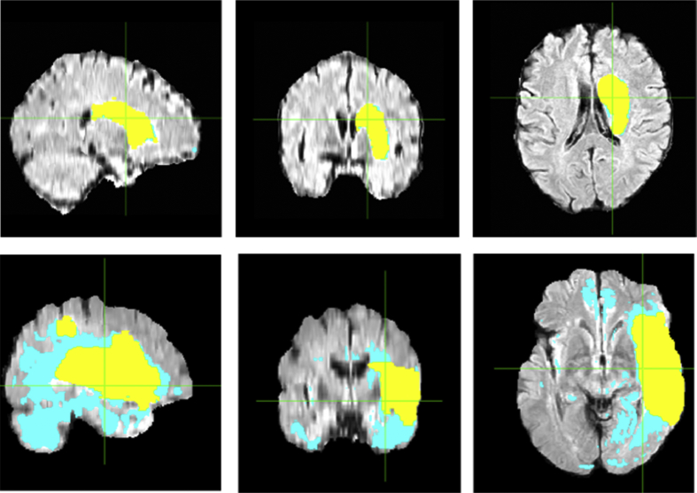
Fig. 1 shows the brain lesion segmentation using K-means. The best performance (Fig. 1 top row) shows that the estimated lesion regions (light blue) and the ground truth (yellow) match very well with the accuracy of 99.27%. The accuracy of K-means varies from subject to subject. And for some subject, the accuracy is only 56.96% (Fig. 1 bottom row).
Fig. 1.
Brain lesion segmentation using K-means. A representative brain lesion segmented using K-means with accuracy of 99.27% (top row). Yellow colored mask is ground truth, while is overlaid on top of the estimated label in blue. A representative lesion segmentation using K-means with accuracy of 56.96% (bottom row).
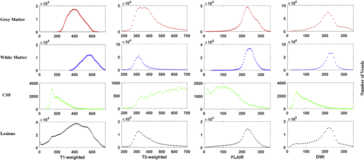
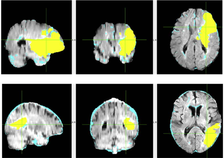
GMM-EM is applied to segment brain lesion, since in each MRI image modality, the intensity of four different brain tissues follows Gaussian distribution approximately as shown in Fig. 2. The segmentation shows GMM-EM works well with the average accuracy of 85%. The estimated lesion regions (light blue) matches the ground truth lesion regions (yellow) well for the best performance subject (Fig. 3 top row) with the accuracy of 95%. While for some subjects, GMM-EM does not segment lesion correctly with healthy regions misclassified as lesion regions. Fig. 3 bottom row shows representative subject with accuracy of 89.02% and the edge of the brain is misclassified as lesion.
Fig. 2.
Signal intensity histogram of GM, WM, CSF, and lesion (if present) in T1-weighted, T2-weighted, FLAIR, and DWI MRI of a representative subject.
Fig. 3.
GMM-EM brain segmentation visualization. The best performance (top row) of GMM-EM have the accuracy of 95% and representative subject with accuracy of 89.02% (bottom row) shows GMM-EM misclassifies edge of the brain as lesion.
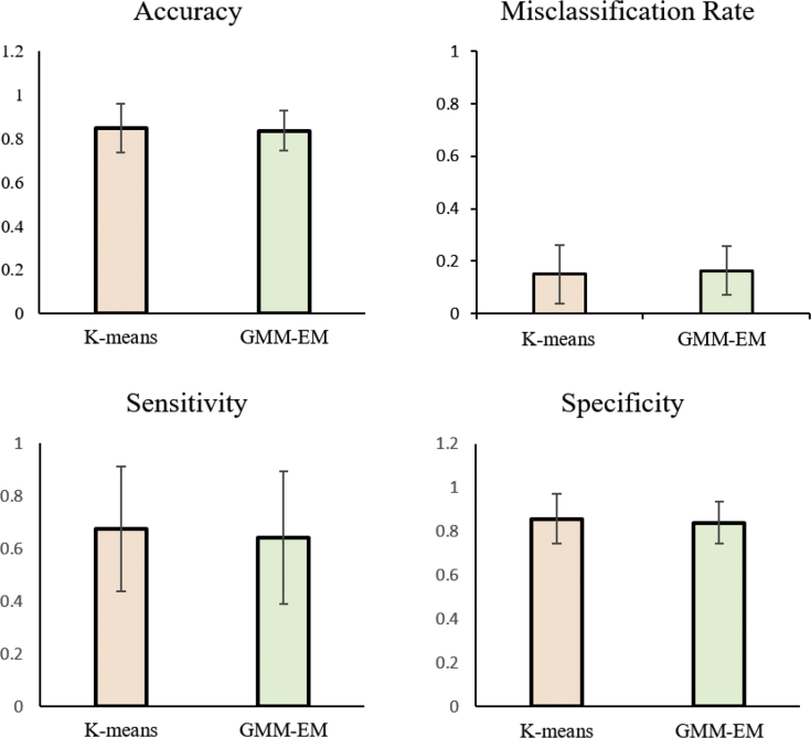
The performance metrics (accuracy, misclassification rate, sensitivity, specificity, and false positive rate) were calculated for both K-means and GMM as shown in Fig. 4. The accuracy, sensitivity, and specificity of K-means are 85 ± 11%, 67 ± 24%, and 86 ± 11% specifically. The accuracy, sensitivity, and specificity of GMM-EM are 84 ± 9%, 64 ± 25%, and 84 ± 10% specifically. There is no significant difference between K-means performance and GMM-EM performance (p-values of accuracy, sensitivity and specificity are: 0.6645, 0.7647, 0.5479). In addition, both K-means and GMM-EM performance varies from subject to subject.
Fig. 4.
Algorithm performance evaluation and comparison. There is no significant difference between K-means and GMM-EM in accuracy, sensitivity, and specificity.
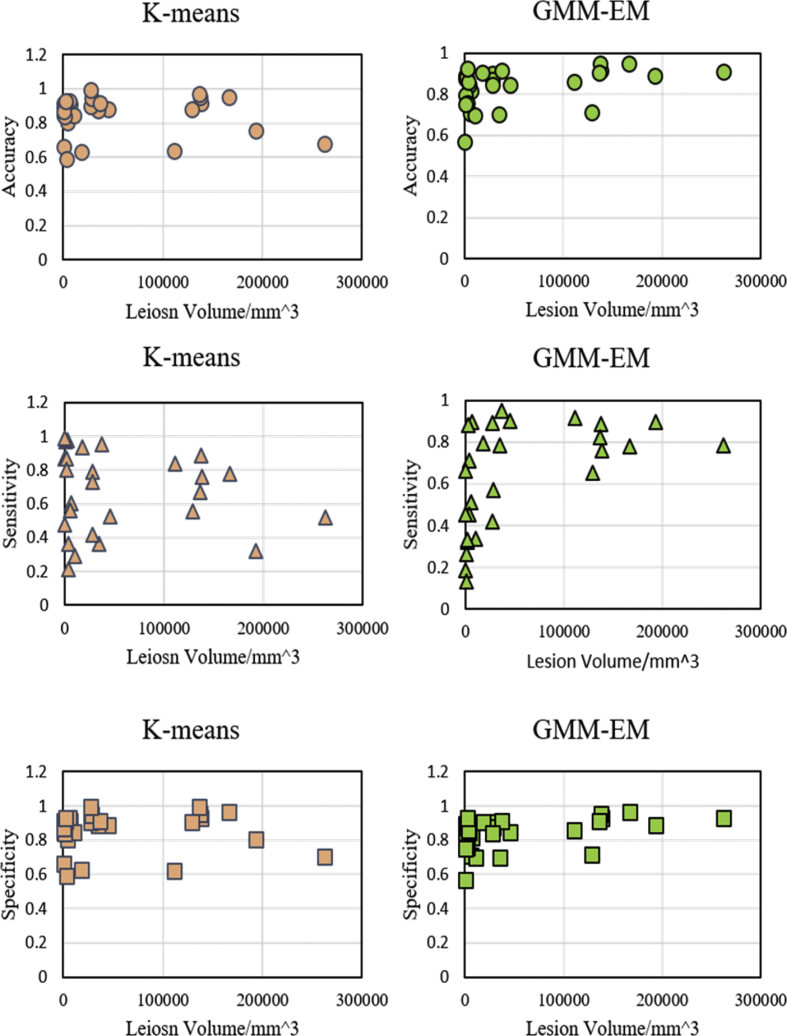
When the algorithms were first applied to perform lesion segmentation, the intuition might suggest that the bigger the lesion size, the better the algorithms performance. However, Fig. 5 shows that there is little correlation between algorithms performance accuracy (sensitivity, and specificity) and the lesion volume. In Fig. 5, the lesion volumes were calculated by counting the number voxels labeled as lesion in mask imaging.
Fig. 5.
Lesion size does not affect the performance of K-means and GMM-EM algorithms.
2. Experimental design, materials, and methods
2.1. Data and feature extraction
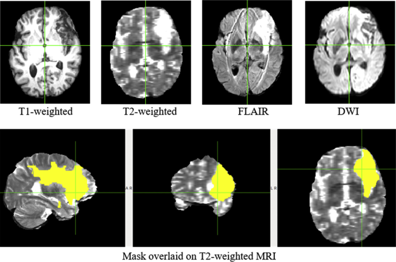
Raw data were acquired from ischemic stroke lesion segmentation 2015 online database [2] (http://www.isles-challenge.org/ISLES2015/), and data is one of the two sub-taskes: sub-acute ischemic stroke lesion segmentation (SISS) training data with 28 subjects. Each of the 28 subjects contains T1-weighted, T2-weighted, FLAIR, DWI images and a lesion mask labeled by experts as ground truth as shown in Fig. 6.
Fig. 6.
MRI data acquired from ischemic stroke lesion segmentation 2015 online database. Images from 4 MRI modalities, T1-weighted, T2-weighted, FLAIR, and DWI, are available (first row), along with mask (ground truth in yellow) overlaid on T2-weighted image in different views (second row).
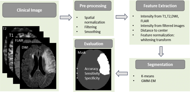
The flowchart of the work is shown in Fig. 7. After data were acquired, pre-processing was performed to make sure different images are in the same space. Then, features were extracted and normalized. K-means and GMM-EM were used to segment lesion from the rest of the brain tissue. Algorithms performance were evaluated by comparing the estimated lesion region with mask (ground truth).
Fig. 7.
Flowchart of lesion segmentation in MRI. Four kinds of images from T1-weighted, T2-weighted, FLAIR and DWI MRI modalities were acquired and pre-processed, then features were extracted. K-means and GMM-EM algorithms were used to segment Lesion. Algorithms performance were evaluated by confusion matrix.
In the pre-processing step, all images were co-registered to the standard space using MNI152 1 mm symmetric human brain atlas. In addition, for each MRI modality, images were intensity-normalized based on the average across all subjects so that features were consistent.
For each voxel, 25 features are extracted to feed into K-means and GMM-EM algorithms. The first four features are the signal intensity from T1-weighted, T2-weighted, FLAIR, DWI images. The next four are the intensities from the smoothed T1-weighted, T2-weighted, FLAIR, DWI images using a Gaussian kernel with sigma of 3 mm. Then the local information of each voxel within the brain mask is obtained using an 11 mm × 11 mm x 11mm cubic window of neighboring voxels centered at this voxel. More specifically, among more than 1 million voxels per subject, the mean, median, variance, 10th percentile and 90th percentile are calculated as four individual features for each voxel from its ±5 mm neighbors of 1330 voxels. These parameters contribute to features 9th through 24th features. The last feature was the distance of each voxel to the image center.
2.2. K-means clustering
K-means classifies n observations into clusters with the aim at minimizing the distance function:
Where represents the th.
Cluster center.
The K-means algorithm:
-
1.
Initialize cluster centroids with random samples;
-
2.
Assign each observation to the nearest cluster center;
-
3.
Recalculate and update each cluster center ; where is the number of elements in the th cluster;
-
4.
Repeat steps 2 and 3 until does not change.
Here, in this paper, we assign voxels into 4 groups: white matter (WM), gray matter (GM), cerebrospinal fluid (CSF), and lesion if present.
2.3. Gaussian mixture model-expectation maximization
In regions where MRI signal is present with signal-to-noise (SNR) ≥ 3, noise follows a Gaussian distribution approximately [[3], [4], [5]]. The histogram of brain MRI with noise in presence can be represented by a Gaussian Mixture Model in which each tissue type such as white matter, gray matter, cerebrospinal fluid, lesion if present follows a Gaussian distribution. In this model, each voxel is assigned to one of the classes.
Gaussian mixture model can be defined as:
Where is a d-dimensional observation vector, are the mixture weights that satisfy and , and is a d-variate Gaussian density for the th mixture component as given by the equation:
where is the th mean vector and is the th covariance matrix.
The parameters (including means, covariances and weights of each component) can be determined by maximizing the likelihood function.
EM Algorithm.
-
1.
Initialize means, covariances and the mixing coefficients and evaluate the initial value of the log likelihood.
-
2.
E step. Evaluate the posterior probability using the current parameter
-
3.
M step. Recalculate the parameters using the current posterior and update the parameters
where
-
4.
Evaluate the log likelihood
-
5.
Repeat step 2, 3, and 4 until the convergence criterion is satisfied.
Acknowledgments
The authors acknowledge the invaluable support from Ischemic Stroke Lesion Segmentation.
Conflict of Interest
The authors declare that they have no known competing financial interests or personal relationships that could have appeared to influence the work reported in this paper.
References
- 1.van de Ven A.L. Nanoformulation of olaparib amplifies PARP inhibition and sensitizes PTEN/TP53-Deficient prostate cancer to radiation. Mol. Cancer Ther. 2017;16(7):1279–1289. doi: 10.1158/1535-7163.MCT-16-0740. [DOI] [PMC free article] [PubMed] [Google Scholar]
- 2.Maier O. Isles 2015 – a public evaluation benchmark for ischemic stroke lesion segmentation from multispectral MRI. Med. Image Anal. 2017;35:250–269. doi: 10.1016/j.media.2016.07.009. [DOI] [PMC free article] [PubMed] [Google Scholar]
- 3.Despotovic I., Goossens B., Philips W. MRI segmentation of the human brain: challenges, methods, and applications. Comput. Math Methods Med. 2015;2015:450341. doi: 10.1155/2015/450341. [DOI] [PMC free article] [PubMed] [Google Scholar]
- 4.Gudbjartsson H., Patz S. The Rician distribution of noisy MRI data. Magn. Reson. Med. 1995;34(6):910–914. doi: 10.1002/mrm.1910340618. [DOI] [PMC free article] [PubMed] [Google Scholar]
- 5.Gharagouzloo C.A. Quantitative vascular neuroimaging of the rat brain using superparamagnetic nanoparticles: new insights on vascular organization and brain function. Neuroimage. 2017;163:24–33. doi: 10.1016/j.neuroimage.2017.09.003. [DOI] [PMC free article] [PubMed] [Google Scholar]


