Weak signals in high-dimension regression: detection, estimation and prediction

Summary.

Regularization methods, including Lasso, group Lasso and SCAD, typically focus on selecting variables with strong effects while ignoring weak signals. This may result in biased prediction, especially when weak signals outnumber strong signals. This paper aims to incorporate weak signals in variable selection, estimation and prediction. We propose a two-stage procedure, consisting of variable selection and post-selection estimation. The variable selection stage involves a covariance-insured screening for detecting weak signals, while the post-selection estimation stage involves a shrinkage estimator for jointly estimating strong and weak signals selected from the first stage. We term the proposed method as the covariance-insured screening based post-selection shrinkage estimator. We establish asymptotic properties for the proposed method and show, via simulations, that incorporating weak signals can improve estimation and prediction performance. We apply the proposed method to predict the annual gross domestic product (GDP) rates based on various socioeconomic indicators for 82 countries.

1. Introduction

Given n independent samples, we consider a high-dimensional linear regression model

$$y=X\mathit{\beta }+\epsilon ,$$ (1)

where y = (y₁, … , y_n)^T is an n-vector of responses, X = (X_ij)_n×p is an n × p random design matrix, β = (β₁, …, β_p)^T is a p-vector of regression coefficients and ε = (ε₁, … , ε_n)^T n is an n-vector of independently and identically distributed random errors with mean 0 and variance σ². Let ${\beta }^{*}={\left({\beta }_1^{*},\dots ,{\beta }_p^{*}\right)}^{\text{T}}$ denote the true value of β. We write X = (x⁽¹⁾, …, x⁽ⁿ⁾)^T = (x₁, …, x_p), where x⁽ⁱ⁾ = (X_ij, … , X_ip)^T is the i-th row of X and x_j is the j-th column of X, for i = 1, …, n and j = 1, …, p. Without the subject index i, we write y, X_j and ε as the random variables underlying y_i, X_ij and ε_i, respectively. We assume that each X_j is independent of ε. We write x as the random vector underlying x⁽ⁱ⁾ and assume that x follows a p-dimensional multivariate sub-Gaussian distribution with mean zeros, variance proxy ${\sigma }_x^2$, and covariance matrix Σ. Sub-Gaussian distributions contain a wide class of distributions such as Gaussian, binary and all bounded random variables. Therefore, our proposed framework can accommodate more data types, as opposed to the conventional Gaussian distributions.

We assume that model (1) is sparse. That is, the number of nonzero β* components is less than n. When p > n, the essential problem is to recover the set of predictors with nonzero coefficients. The past two decades have seen many regularization methods developed for variable selection and estimation in high-dimensional settings, including Lasso (Tibshirani, 1996), adaptive Lasso (Zou, 2006), group Lasso (Yuan and Lin, 2006), SCAD (Fan and Li, 2001) and MCP (Zhang, 2010), among many others. Most regularization methods assume the restrictive β-min condition which requires that the strength of nonzero ${\beta }_j^{*}$′s is larger than a certain noise level (Zhang and Zhang, 2014). Hence, regularization methods may fail to detect weak signals with nonzero but small ${\beta }_j^{*}$′s, and this will result in biased estimates and inaccurate predictions, especially when weak signals outnumber strong signals.

Detection of weak signals is challenging. However, if weak signals are partially correlated with strong signals which satisfy the β-min condition, they may be more reliably detected. To elaborate on this idea, first notice that the regression coefficient ${\beta }_j^{*}$ can be written as

$${\beta }_j^{*}=\sum _{1\le j^{\prime }\le p}{\Omega }_{j{j}^{\prime }}\text{ cov}\left(X_{j^{\prime }},y\right),j=1,\dots ,p,$$ (2)

where Ω_jj′ is the jj^′-th entry of of Ω = Σ⁻¹, the precision matrix of x. Let ρ_jj′ be the partial correlation of X_j and X_j′, i.e. the correlation between the residuals of X_j and X_j′ after regressing them on all the other X variables. It can be shown that ${\rho }_{j{j}^{\prime }}=-{\Omega }_{j{j}^{\prime }}/\sqrt{{\Omega }_{jj}{\Omega }_{j^{\prime }{j}^{\prime }}}$. Hence, that X_j and X_j′ are partially uncorrelated is equivalent to Ω_jj′ = 0. Assume that Ω is a sparse matrix with only a few nonzero entries in Ω. When the right hand side of (2) can be accurately evaluated, weak signals can be distinguished from those of noises. In high-dimensional settings, it is impossible to accurately evaluate ${\sum }_{1\le j^{\prime }\le p}{\Omega }_{j{j}^{\prime }}\text{cov }\left(X_{j^{\prime }},y\right)$. However, under the faithfulness condition that will be introduced in Section 3, a variable, say, indexed by j′, satisfing the β-min condition will have a nonzero cov(X_j′, y). Once we identify such strong signals, we set to discover variables that are partially correlated with them.

For brevity, we term weak signals which are partially correlated with strong signals as “weak but correlated” (WBC) signals. This paper aims to incorporate WBC signals in variable selection, estimation and prediction. We propose a two-stage procedure which consists of variable selection and post-selection estimation. The variable selection stage involves a covariance-insured screening for detecting weak signals, and the post-selection estimation stage involves a shrinkage estimator for jointly estimating strong and weak signals selected from the first stage. We call the proposed method as the covariance-insured screening based post-selection shrinkage estimator (CIS-PSE). Our simulation studies demonstrate that by incorporating WBC signals, CIS-PSE improves estimation and prediction accuracy. We also establish the asymptotic selection consistency of CIS-PSE.

The paper is organized as follows. We outline the proposed CIS-PSE method in Section 2 and investigate its asymptotic properties in Section 3. We evaluate the finite-sample performance of CIS-PSE via simulations in Section 4, and apply the proposed method to predict the annual gross domestic product (GDP) rates based on the socioeconomic status for 82 countries in Section 5. We conclude the paper with a brief discussion in Section 6. All technical proofs are provided in Appendix.

2. Methods

2.1. Notation

We use scripted upper-case letters, such as S, to denote the subsets of {1, … , p}. Denote by $\left|\mathcal{S}\right|$ the cardinality of $\mathcal{S}$ and by ${\mathcal{S}}^c$ the complement of $\mathcal{S}$. For a vector v, we denote a subvector of v indexed by $\mathcal{S}$ by $v_{\mathcal{S}}$. Let $X_{\mathcal{S}}=\left(x_j,j\in \mathcal{S}\right)$ be a submatrix of the design matrix X restricted to the columns indexed by $\mathcal{S}$. For the symmetric covariance matrix Σ, denote by ${\Sigma }_{\mathcal{S}{\mathcal{S}}^{\prime }}$ its submatix with the row and column indices restricted to subsets $\mathcal{S}$ and ${\mathcal{S}}^{\prime }$, respectively. When $\mathcal{S}={\mathcal{S}}^{\prime }$, we write ${\Sigma }_{\mathcal{S}}={\Sigma }_{\mathcal{S}{\mathcal{S}}^{\prime }}$ for short. The notation also applies to its sample version $\widehat{\Sigma }$.

Denote by $\mathcal{G}(\mathcal{V},\mathcal{E};\Omega )$ the graph induced by Ω, where the node set is $\mathcal{V}=\left\{1,\dots ,p\right\}$ and the set of edges is denoted by $\mathcal{E}$. An edge is a pair of nodes, say, k and k′, with Ω_kk′ ≠ 0. For a subset ${\mathcal{V}}_l\subset \mathcal{V}$, denote by Ω_l the principal submatrix of Ω with its row and column indices restricted to ${\mathcal{V}}_l$ and by ${\mathcal{E}}_l$ the corresponding edge set. The subgraph $\mathcal{G}({\mathcal{V}}_l,{\mathcal{E}}_l;{\Omega }_l)$ is a connected component of $\mathcal{G}(\mathcal{V},\mathcal{E};\Omega )$ if (i) any two nodes in ${\mathcal{V}}_l$ are connected by edges in ${\mathcal{E}}_l$; (ii) for any node $k\in {\mathcal{V}}_l^c$, there exists a node $k^{\prime }\in {\mathcal{V}}_l$ such that k, k′ cannot be connected by any edges in $\mathcal{E}$.

For a symmetric matrix A, denote by tr(A) the trace of A, and denote by λ_min(A) and λ_max(A) the minimum and maximum eigenvalues of A. We define the operator norm and the Frobenius norm as $\Vert A\Vert ={\lambda }_{\text{max}}^{1/2}\left(A^{\text{T}}A\right)$ and $\Vert A{\Vert }_F=tr{\left(A^{\text{T}}A\right)}^{1/2}$, respectively. For a p-vector v, denote its L_q norm by $\Vert v{\Vert }_q={\left({\sum }_{j=1}^p{\left|v_j\right|}^q\right)}^{1/q}$ with q ≥ 1. For two real numbers a and b, denote a∨b = max(a, b).

Denote the sample covariance matrix and the marginal sample covariance between X_j and y, j = 1, …, p, by

$$\widehat{\Sigma }=\frac{1}{n}\sum _{i=1}^n{\text{x}}^{(i)}{\left({\text{x}}^{(i)}\right)}^{\text{T}}\text{ and }\widehat{\text{ cov }}\left(X_j,y\right)=\frac{1}{n}\sum _{i=1}^n{X}_{ij}{y}_i.$$

For a vector V = (V₁, …,V_p)^T, denote $\widehat{\text{ cov }}(V,y)={\left(\widehat{\text{ cov }}\left(V_1,y\right),\dots ,\widehat{\text{ cov }}\left(V_p,y\right)\right)}^{\text{T}}$.

2.2. Defining strong and weak signals

Consider a low-dimensional linear regression model where p < n. The ordinary least squares (OLS) estimator ${\widehat{\beta }}^{\text{OLS}}={\widehat{\Sigma }}^{-1}\widehat{\text{ cov }}(x,y)=\widehat{\Omega }\widehat{\text{ cov }}(x,y)$ minimizes the prediction error, where $\widehat{\Omega }={\widehat{\Sigma }}^{-1}$ is the empirical precision matrix. It is also known that ${\widehat{\beta }}^{\text{OLS}}$ is an unbiased estimator of β* and yields the best outcome prediction ${\widehat{y}}^{\text{best }}=X\widehat{\Omega }\widehat{\text{ cov }}(x,y)$ with the minimal prediction error.

However, when p > n, $\widehat{\Sigma }$ becomes non-invertible, and thus β Cannot be estimated using all X variables. Let ${\mathcal{S}}_0=\left\{j:{\beta }_j^{*}\ne 0\right\}$ be the true signal set and assume that $\left|{\mathcal{S}}_0\right|<n$. If $\mathcal{S}$ were known, the predicted outcome, ${\widehat{y}}^{\text{best}}=X_{{\mathcal{S}}_0}{\widehat{\Sigma }}_{{\mathcal{S}}_0}^{-1}\widehat{\text{ cov }}\left(x_{{\mathcal{S}}_0},y\right)$, would have the smallest prediction error. In practice, ${\mathcal{S}}_0$ is unknown and some variable selection method must be applied first to identify ${\mathcal{S}}_0$. We define the set of strong signals as

$${\mathcal{S}}_1=\left\{j:|{\beta }_j^{*}|>c\sqrt{\text{log}p/n}\text{ for some }c>0,1\le j\le p\right\}$$ (3)

and let ${\mathcal{S}}_2={\mathcal{S}}_0\backslash {\mathcal{S}}_1$ be the set of weak signals. Then, the OLS estimator and the best outcome prediction are given by

$${\widehat{\beta }}^{\text{OLS}}=\left(\begin{array}{c}{\widehat{\beta }}_{{\mathcal{S}}_1}^{\text{OLS}}\\ {\widehat{\beta }}_{{\mathcal{S}}_2}^{\text{OLS}}\end{array}\right)=\left(\begin{array}{c}{\widehat{\mathbf{\Omega }}}_{11}\widehat{\text{ cov }}\left(x_{{\mathcal{S}}_1},y\right)+{\widehat{\mathbf{\Omega }}}_{12}\widehat{\text{ cov }}\left(x_{{\mathcal{S}}_2},y\right)\\ {\widehat{\mathbf{\Omega }}}_{21}\widehat{\text{ cov }}\left(x_{{\mathcal{S}}_1},y\right)+{\widehat{\mathbf{\Omega }}}_{22}\widehat{\text{ cov }}\left(x_{{\mathcal{S}}_2},y\right)\end{array}\right)$$

and

$${\widehat{y}}^{\text{ best }}=X_{{\mathcal{S}}_1}{\widehat{\mathbf{\Omega }}}_{11}\widehat{\text{ cov }}\left(x_{S_1},y\right)+X_{S_2}{\widehat{\mathbf{\Omega }}}_{21}\widehat{\text{ cov }}\left(x_{{\mathcal{S}}_1},y\right)+{\mathbf{\text{X}}}_{{\mathcal{S}}_1}{\widehat{\mathbf{\Omega }}}_{12}\widehat{\text{ cov }}\left({\mathbf{\text{x}}}_{\mathcal{S}}{}_2,y\right)+{\mathbf{\text{X}}}_{{\mathcal{S}}_2}{\widehat{\mathbf{\Omega }}}_{22}\widehat{\text{ cov }}\left({\mathbf{\text{x}}}_{S_2},y\right),$$

where $\left(\begin{array}{cc}{\widehat{\Omega }}_{11}& {\widehat{\Omega }}_{12}\\ {\widehat{\Omega }}_{21}& {\widehat{\Omega }}_{22}\end{array}\right)={\left(\begin{array}{cc}{\widehat{\Sigma }}_{{\mathcal{S}}_1}& {\widehat{\Sigma }}_{{\mathcal{S}}_1{\mathcal{S}}_2}\\ {\widehat{\Sigma }}_{{\mathcal{S}}_2{\mathcal{S}}_1}& {\widehat{\Sigma }}_{{\mathcal{S}}_2}\end{array}\right)}^{-1}$ is the partitioned empirical precision matrix. We observe that the partial Correlations between the variables in ${\mathcal{S}}_1$ and ${\mathcal{S}}_2$ contribute to the estimation of ${\beta }_{{\mathcal{S}}_1}$ and ${\beta }_{{\mathcal{S}}_2}$, and outcome prediction. Therefore, incorporating WBC signals helps reduce the estimation bias and prediction error.

We now further divide ${\mathcal{S}}_2$ into ${\mathcal{S}}_{\text{WBC}}$ and ${\mathcal{S}}_{2*}$. Here, ${\mathcal{S}}_{\text{WBC}}$ is the set of weak signals which have nonzero partial correlations with the signals in ${\mathcal{S}}_1$ and ${\mathcal{S}}_{2*}$ is the set of weak signals which are not partially orrelated with signals in ${\mathcal{S}}_1$. Formally, with c given in (3),

$${\mathcal{S}}_{\text{WBC}}=\left\{j:0<|{\beta }_j^{*}|<c\sqrt{\text{log}p/n}\text{ and }{\Omega }_{j{j}^{\prime }}\ne 0\text{ for some }{j}^{\prime }\in {\mathcal{S}}_1,1\le j\le p\right\}$$

and

$${\mathcal{S}}_{2*}=\left\{j:0<|{\beta }_j^{*}|<c\sqrt{\text{log}p/n}\text{ and }{\Omega }_{j{j}^{\prime }}=0\text{ for any }{j}^{\prime }\in {\mathcal{S}}_1,1\le j\le p\right\}.$$

Thus, p predictors can be partitioned as ${\mathcal{S}}_1\cup {\mathcal{S}}_{\text{WBC}}\cup {\mathcal{S}}_{2*}\cup {\mathcal{S}}_{\text{null}}=\left\{1,\dots ,p\right\}$, where ${\mathcal{S}}_{\text{null}}=\left\{j:{\beta }_j^{*}=0\right\}$. We assume that $|{\mathcal{S}}_1|=p_1,|{\mathcal{S}}_{\text{WBC}}|=p_{\text{WBC}}$ and $|{\mathcal{S}}_{2*}|=p_{2*}$.

2.3. Covariance-insured screening based post-selection shrinkage estimator (CIS-PSE)

Our proposed CIS-PSE method consists of the variable selection and post-shrinkage estimation steps.

Variable selection:

First, we detect strong signals by regularization methods such as Lasso or adaptive Lasso. Denote by $\widehat{{\mathcal{S}}_1}$ the set of detected strong signals. To identify WBC signals, we evaluate (2) for each $j\in {\widehat{\mathcal{S}}}_1^c$. When there is no confusion, we use a j′ to denote a strong signal.

Though estimating cov(X_j′, y) for every 1 ≤ j′ ≤ p can be easily done, identifying and estimating nonzero entries in Ω is still challenging in high-dimensional settings. However, for identifying WBC signals, it is unnecessary to estimate the whole Ω matrix. Leveraging intra-feature correlations among predictors, we introduce a computationally efficient method for detecting nonzero Q_jj′’s.

Variables that are partially correlated with signals in $\widehat{{\mathcal{S}}_1}$ form the connected components of $\mathcal{G}(\mathcal{V},\mathcal{E};\Omega )$ that contain at least one element of $\widehat{{\mathcal{S}}_1}$. Therefore, for detecting WBC signals, it suffices to focus on such connected components. Under the sparsity assumptions of β* and Ω, the size of such connected components is relatively small. For example, as shown in Figure 1, the first two diagonal blocks of a moderate size are relevant for detection of WBC signals.

Figure 1:

An illustrative example of marginally strong signals and their connected components in $\mathcal{G}(\mathcal{V},\mathcal{E};\Omega )$. Left panel: structure of Ω; Middle panel: structure of Ω after properly reordering the row and column indices of Ω; Right panel: the corresponding graph structure and connected components of the strong signals. Signals in ${\mathcal{S}}_1$ are colored red. Signals in ${\mathcal{S}}_{2*}$ are colored orange. WBC signals in ${\mathcal{S}}_{\text{WBC}}$ are colored yellow.

Under the sparsity assumption of Ω, the connected components of Ω can be inferred from those of the thresholded sample covariance matrix (Mazumder and Hastie, 2012; Bickel and Levina, 2008; Fan et al., 2011; Shao et al., 2011), which is much easier to estimate and can be calculated in a parallel manner. Denote by ${\tilde{\Sigma }}^{\alpha }$ the thresholded sample covariance matrix with a thresholding parameter α, where ${\tilde{\Sigma }}_{k{k}^{\prime }}^{\alpha }={\widehat{\Sigma }}_{k{k}^{\prime }}1\left\{|{\widehat{\Sigma }}_{k{k}^{\prime }}|\ge \alpha \right\},1\le k,k^{\prime }\le p$ with 1(·) being the indicator function. Denote by $\mathcal{G}\left(\mathcal{V},\tilde{\mathcal{E}};{\tilde{\Sigma }}^{\alpha }\right)$ the graph corresponding to ${\tilde{\Sigma }}^{\alpha }$. For variable k, 1 ≤ k ≤ p, denote by ${\mathcal{C}}_{[k]}$ the vertex set of the connected component in $\mathcal{G}(\mathcal{V},\mathcal{E};\Omega )$ containing k. If variables k and k′ belong to the same connected component, 1 ≤ k ≠ k′ ≤ p, then ${\mathcal{C}}_{[k]}={\mathcal{C}}_{\left[k^{\prime }\right]}$. For example, ${\mathcal{C}}_{[14]}={\mathcal{C}}_{[16]}={\mathcal{C}}_{[24]}={\mathcal{C}}_{[26]}={\mathcal{C}}_{[29]}$ in the third panel of Figure 1. Clearly, when $k^{\prime }\notin {\mathcal{C}}_{[k]},{\Omega }_{k{k}^{\prime }}=0$, evaluating (2) is equivalent to estimating

$${\beta }_j^{*}=\sum _{j^{\prime }\in {\mathcal{C}}_{[j]}}{\Omega }_{j{j}^{\prime }}\text{ cov }\left(X_{j^{\prime }},y\right),j=1,\dots ,p.$$ (4)

Correspondingly, for a variable k, 1 ≤ k ≤ p, denote by ${\widehat{\mathcal{C}}}_{[k]}$ the vertex set of the connected component in $\mathcal{G}\left(\mathcal{V},\tilde{\mathcal{E}};{\tilde{\Sigma }}^{\alpha }\right)$ containing k. For a multivariate Gaussian x, Mazumder and Hastie (2012) showed that ${\mathcal{C}}_{[k]}$ ′s can be exactly recovered from ${\mathcal{C}}_{[k]}$ ′s with a properly chosen α. For a multivariate sub-Gaussian x, we refer to the following lemma.

Lemma 2.1. Suppose that the maximum size of a connected component in Ω containing a variable in ${\mathcal{S}}_0$ is of order O(exp(n^ξ)), for some 0 < ξ < 1, then under Assumption (A7) specified in Section 3, with an $\alpha =O\left(\sqrt{n^{\xi -1}}\right)$ and for any variable k, 1 ≤ k ≤ p, we have

$$P\left({\mathcal{C}}_{[k]}={\widehat{\mathcal{C}}}_{[k]}\right)\ge 1-C_1{n}^{\xi }\text{exp}\left(-C_2{n}^{1+\xi }\right)\to 1$$ (5)

for some positive constants C₁ and C₂.

We summarize the variable selection procedure for ${\mathcal{S}}_1$ and ${\mathcal{S}}_{\text{WBC}}$.

Step S1: Detection of ${\mathcal{S}}_1$. Obtain a candidate subset $\widehat{{\mathcal{S}}_1}$ of strong signals using a penalized regression method. Here, we consider the penalized least squares (PLS) estimator from Gao et al. (2017):

$${\widehat{\beta }}^{\text{PLS}}=\underset{\beta }{\text{argmin}}\left\{\Vert y-X\beta {\Vert }_2^2+\sum _{j=1}^p{\text{Pen}}_{\lambda }\left({\beta }_j\right)\right\},$$ (6)

where Pen_λ(β_j) is a penalty on each individual β_j to shrink the weak effects toward zeros and select the strong signals, with the tuning parameter λ > 0 controlling the size of the candidate subset $\widehat{{\mathcal{S}}_1}$. Commonly used penalties are Pen_λ(β_j) = λ|β_j| and Pen_λ(β_j) = λω_j |β_j| for Lasso and adaptive Lasso, where ω_j > 0 is a known weight.

Step 2: Detection of ${\mathcal{S}}_{WBC}$. First, for a given threshold α, construct a sparse estimate of the covariance matrix ${\tilde{\Sigma }}^{\alpha }$. Next, for each selected variable j′ in $\widehat{{\mathcal{S}}_1}$ from Step S1, detect ${\widehat{\mathcal{C}}}_{\left[j^{\prime }\right]}$, the node set, corresponding to its connected component in $\mathcal{G}\left(\mathcal{V},\tilde{\mathcal{E}};{\tilde{\Sigma }}^{\alpha }\right)$. Let $\mathcal{U}\left(\alpha ,{\widehat{\mathcal{S}}}_1\right)$ be the union of the vertex sets corresponding to those connected components detected. That is, $\mathcal{U}\left(\alpha ,{\widehat{\mathcal{S}}}_1\right)={\cap }_{j^{\prime }\in {\widehat{\mathcal{S}}}_1}{\widehat{\mathcal{C}}}_{\left[j^{\prime }\right]}$. Then according to (4), it suffices to identify WBC signals within $\mathcal{U}\left(\alpha ,{\widehat{\mathcal{S}}}_1\right)$. Specifically, for each $j\in {\widehat{\mathcal{S}}}_1^c\cap \mathcal{U}\left(\alpha ,{\widehat{\mathcal{S}}}_1\right)$, let ${\tilde{\Sigma }}_{[j]}^{\alpha }$ be the submatrix from restricting ${\tilde{\Sigma }}^{\alpha }$ on ${\widehat{\mathcal{C}}}_{\left[j\right]}$. We then evaluate (4) and select WBC variables by

$${\widehat{\mathcal{S}}}_{\text{WBC}}=\left\{j\in {\widehat{\mathcal{S}}}_1^c\cap \mathcal{U}\left(\alpha ,{\widehat{\mathcal{S}}}_1\right):\left|\sum _{j^{\prime }\in {\widehat{\mathcal{C}}}_{[j]}}{\left({\tilde{\Sigma }}_{[j]}^{\alpha }\right)}_{j{j}^{\prime }}^{-1}\widehat{\text{ cov }}\left(X_{j^{\prime }},y\right)\right|\ge {\nu }_n\right\}$$ (7)

for some pre-specified ν_n. Here ${\left({\tilde{\Sigma }}_{[j]}^{\alpha }\right)}_{j{j}^{\prime }}^{-1}$ denotes the entry of ${\left({\tilde{\Sigma }}_{[j]}^{\alpha }\right)}^{-1}$ corresponding to variables j and j′. In our numerical studies, we rank the magnitude of variable $j\in {\widehat{\mathcal{S}}}_1^c\cap \mathcal{U}\left(\alpha ,{\widehat{\mathcal{S}}}_1\right)$ according to the magnitude of $|{\sum }_{j^{\prime }\in {\widehat{\mathcal{C}}}_{[j]}}{\left({\tilde{\Sigma }}_{[j]}^{\alpha }\right)}_{j{j}^{\prime }}^{-1}\widehat{\text{ cov }}\left(X_{j^{\prime }},y\right)|$ and select up to the first $n-|{\widehat{\mathcal{S}}}_1|$ variables.

Step 3: Detection of ${\mathcal{S}}_{2*}$. To identify ${\widehat{\mathcal{S}}}_{2*}$, we first solve a regression problem with a ridge penalty only on variables in ${\widehat{\mathcal{S}}}_{1\text{WBC}}^c$, where ${\widehat{\mathcal{S}}}_{1\text{WBC}}={\widehat{\mathcal{S}}}_1\cup {\widehat{\mathcal{S}}}_{\text{WBC}}$. That is,

$${\widehat{\beta }}^{\text{r}}=\underset{\beta }{\text{argmin}}\left\{\Vert y-X\mathit{\beta }{\Vert }_2^2+{\tilde{\lambda }}_n\Vert {\beta }_{{\widehat{\mathcal{S}}}_1^c{}_{\text{WBC}}}{\Vert }_2^2\right\},$$ (8)

where ${\tilde{\lambda }}_n>0$ is a tuning parameter controlling the overall strength of the variables selected in ${\widehat{\mathcal{S}}}_{1\text{WBC}}^c$. Then a post-selection weighted ridge (WR) estimator ${\widehat{\beta }}^{\text{WR}}$ has the form

$${\widehat{\beta }}_j^{\text{WR}}=\{\begin{array}{ll}{\widehat{\beta }}_j^{\text{r}},\hfill & j\in {\widehat{\mathcal{S}}}_{1\text{WBC}},\hfill \\ {\widehat{\beta }}_j^{\text{r}}1\left(|{\widehat{\beta }}_j^{\text{r}}|>a_n\right),\hfill & j\in {\widehat{\mathcal{S}}}_{1\text{WBC}}^c,\hfill \end{array}$$ (9)

where a_n is a thresholding parameter. Then the candidate subset ${\widehat{\mathcal{S}}}_{2*}$ is obtained by

$${\widehat{\mathcal{S}}}_{2*}=\left\{j\in {\widehat{\mathcal{S}}}_{1\text{WBC}}^c:{\widehat{\beta }}_j^{\text{WR}}\ne 0,1\le j\le p\right\}.$$ (10)

Post-selection shrinkage estimation:

We consider the following two cases when performing the post-selection shrinkage estimation.

Case 1: ${\widehat{p}}_1+{\widehat{p}}_{WBC}+{\widehat{p}}_{2*}<n$. We obtain the CIS-PSE on ${\widehat{\mathcal{S}}}_0$ by

$${\widehat{\beta }}_{{\widehat{\mathcal{S}}}_0}^{\text{CIS}-\text{PSE}}={\widehat{\mathbf{\Sigma }}}_{{\widehat{\mathcal{S}}}_0}^{-1}\widehat{\text{ cov }}\left(x_{{\widehat{\mathcal{S}}}_0},y\right),$$ (11)

where ${\widehat{\mathcal{S}}}_0={\widehat{\mathcal{S}}}_1\cup {\widehat{\mathcal{S}}}_{\text{WBC}}\cup {\widehat{\mathcal{S}}}_{2*}$. Then ${\widehat{\beta }}_{{\widehat{\mathcal{S}}}_1}^{\text{ClS}-\text{PSE}}$ and ${\widehat{\beta }}_{{\widehat{S}}_{\text{WBC}}}^{\text{CIS}-\text{PSE}}$ can be obtained by restricting ${\widehat{\beta }}_{{\widehat{\mathcal{S}}}_0}^{\text{CIS}-\text{PSE}}$ to ${\widehat{\mathcal{S}}}_1$ and ${\widehat{\mathcal{S}}}_{\text{WBC}}$, respectively.

Case 2: ${\widehat{p}}_1+{\widehat{p}}_{WBC}+{\widehat{p}}_{2*}>n$. Recall that ${\widehat{\beta }}_{{\widehat{\mathcal{S}}}_{1\text{WBC}}}^{\text{WR}}={\left({\widehat{\beta }}_j^{\text{r}},j\in {\widehat{\mathcal{S}}}_{1\text{WBC}}\right)}^{\text{T}}$ and ${\widehat{\beta }}_{{\mathcal{S}}_2}^{\text{WR}}={\left({\widehat{\beta }}_j^{\text{r}}1\left(|{\widehat{\beta }}_j^{\text{r}}|>a_n\right),j\in {\widehat{\mathcal{S}}}_{2*}\right)}^{\text{T}}$. We obtain the CIS-PSE of ${\beta }_{\widehat{\mathcal{S}}}{}_{{}_{1\text{WBC}}}$ by

$${\widehat{\beta }}_{{\widehat{\mathcal{S}}}_{1\text{WBC}}}^{\text{CIS-PSE}}={\widehat{\beta }}_{{\widehat{\mathcal{S}}}_{1\text{WBC}}}^{\text{WR}}-\left(\frac{{\widehat{s}}_2-2}{{\widehat{T}}_n}\wedge 1\right)\left({\widehat{\beta }}_{{\widehat{\mathcal{S}}}_{1\text{WBC}}}^{\text{WR}}-{\widehat{\beta }}_{{\widehat{\mathcal{S}}}_{1\text{WBC}}}^{\text{RE}}\right),$$ (12)

Where ${\widehat{s}}_2=|{\widehat{\mathcal{S}}}_{2*}|$ and ${\widehat{T}}_n$ is as defined by

$${\widehat{T}}_n={\left({\widehat{\beta }}_{{\widehat{\mathcal{S}}}_{2*}}^{\text{WR}}\right)}^{\text{T}}\left(X_{{\widehat{\mathcal{S}}}_{2*}}^{\text{T}}{M}_{{\widehat{\mathcal{S}}}_{1\text{WBC}}}{X}_{{\widehat{\mathcal{S}}}_{2*}}\right){\widehat{\beta }}_{{\widehat{\mathcal{S}}}_{2*}}^{\text{WR}}/{\widehat{\sigma }}^2,$$ (13)

where $M_{{\widehat{\mathcal{S}}}_{1\text{WBC}}}=I_n-X_{{\widehat{\mathcal{S}}}_{1\text{WBC}}}{\left(X_{{\widehat{\mathcal{S}}}_{1\text{WBC}}}^{\text{T}}{X}_{{\widehat{\mathcal{S}}}_{1\text{WBC}}}\right)}^{-1}{X}_{{\widehat{\mathcal{S}}}_{1\text{WBC}}}^{\text{T}}$ and ${\widehat{\sigma }}^2={\sum }_{i=1}^n{\left(y_i-X_{{\widehat{\mathcal{S}}}_2}^{\text{T}}{\widehat{\beta }}_{{\widehat{\mathcal{S}}}_2}^{\text{WR}}\right)}^2/(n-{\widehat{S}}_2)$. If $X_{{\widehat{\mathcal{S}}}_{1\text{WBC}}}^{\text{T}}{X}_{{\widehat{\mathcal{S}}}_{1\text{WBC}}}$ is singular, we replace ${(X_{{\widehat{\mathcal{S}}}_{1\text{WBC}}}^{\text{T}}{X}_{{\widehat{\mathcal{S}}}_{1\text{WBC}}})}^{-1}$ with a generalized inverse. Then ${\widehat{\beta }}_{{\widehat{\mathcal{S}}}_{\text{1}}}^{\text{CIS}-\text{PSE}}$ and ${\widehat{\beta }}_{{\widehat{\mathcal{S}}}_{\text{WBC}}}^{\text{CIS}-\text{PSE}}$ can be obtained by restricting ${\widehat{\beta }}_{{\widehat{\mathcal{S}}}_{\text{1}}}^{\text{CIS}-\text{PSE}}$ to $\widehat{{\mathcal{S}}_1}$ and ${\widehat{\mathcal{S}}}_{\text{WBC}}$, respectively.

Set ${\widehat{\mathcal{S}}}_{\text{null}}={\left({\widehat{\mathcal{S}}}_1\cup {\widehat{\mathcal{S}}}_{\text{WBC }}\cup {\widehat{\mathcal{S}}}_{2*}\right)}^c$. The final CIS-PSE estimator ${\widehat{\beta }}^{\text{CIS}-\text{PSE}}$ is defined as

$${\widehat{\beta }}^{\text{CIS}-\text{PSE}}={\left({\left({\widehat{\beta }}_{{\widehat{\mathcal{S}}}_1}^{\text{CIS}-\text{PSE}}\right)}^{\text{T}},{\left({\widehat{\beta }}_{{\widehat{S}}_{\text{WBC}}}^{\text{CIS}-\text{PSE}}\right)}^{\text{T}},{\left({\widehat{\beta }}_{{\widehat{\mathcal{S}}}_{2*}}^{\text{WR}}\right)}^{\text{T}},0_{{\widehat{\mathcal{S}}}_{\text{ null }}}\right)}^{\text{T}}.$$ (14)

2.4. Selection of tuning parameters

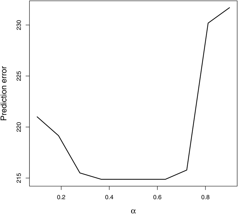
When selecting strong signals, the tuning parameter λ in Lasso or adaptive Lasso can be chosen by BIC (Zou, 2006). To choose ν_n for the selection of WBC signals according to (7), we rank variables $j\in {\widehat{\mathcal{S}}}_1^c\cap \mathcal{U}\left(\alpha ,{\widehat{\mathcal{S}}}_1\right)$ according to the magnitude of $|\sum _{j^{\prime }\in {\widehat{\mathcal{C}}}_{[j]}}{\left({\tilde{\Sigma }}_{[j]}^{\alpha }\right)}_{j{j}^{\prime }}^{-1}\widehat{\text{ cov }}\left(X_{j^{\prime }},y\right)|$ and select the first $r\le n-|{\widehat{\mathcal{S}}}_1|$ variables to be ${\widehat{\mathcal{S}}}_{\text{WBC}}$. Here, r is chosen so that ${\widehat{\mathcal{S}}}_{1\text{WBC}}$ minimizes prediction errors on an independent validation dataset. For tuning parameter α, we set α = c₃ log(n), for some positive constant c₃, as suggested in Shao et al. (2011). Our empirical experiments show that α = c₃ log(n) tends to give the larger true positives and the smaller false positives in identifying WBC variables. Figure 7 in Appendix reveals that in order to find the optimal α that minimizes the prediction error on a validation dataset, it suffices to conduct a grid search with only a few proposed values of α. In our numerical studies, instead of thresholding the sample covariance matrix, we threshold the sample correlation matrix. As correlations are ranged between −1 and 1, it is easier to set a target range for α. To detect signals in ${\mathcal{S}}_{2*}$, we follow Gao et al. (2017) to use cross-validation to choose ${\tilde{\lambda }}_n$ and a_n in (8) and (9), respectively. In particular, we set and ${\tilde{\lambda }}_n=c_1{a}_n^{-2}{(\text{loglog}n)}^3\text{log}(n\vee p)$ a_n = c₂n^−1/8 for some positive constants c₁ and c₂. In the training dataset we fix the tuning parameters and fit the model, and in the validation dataset we compute the prediction error of the model. We repeat this procedure for various c₁ and c₂, and choose a pair that gives the smallest prediction error on the validation dataset.

Figure 7:

Sum of squared prediction error (SSPE) corresponding to different α’s.

3. Asymptotic properties

To investigate the asymptotic properties of CIS-PSE, we assume the following.

(A1) The random error ϵ has a finite kurtosis.

(A2) log(p) = O(n^ν) for some 0 < ν < 1.

(A3) There are positive constants κ₁ and κ₂ such that 0 < κ₁ < λ_miη(Σ) ≤ λ_max(Σ) < κ₂ < ∞.

(A4) Sparse Riesz condition (SRC): For the random design matrix X, any $\mathcal{S}\subset \left\{1,\dots ,p\right\}$ with $|\mathcal{S}|=q,q\le p$, and any vector $v\in {ℝ}^q$, there exist 0 < c_* < c* < ∞ such that $c_{*}\le \Vert X_S^{\text{T}}v{\Vert }_2^2/\Vert v{\Vert }_2^2\le c*$ holds with probability tending to 1.

(A5) Faithfulness Assumption: Suppose that

$$\text{max}|{\Sigma }_{{\mathcal{S}}_1^c{\mathcal{S}}_1}{\beta }_{{\mathcal{S}}_1}^{*}|+\text{max}|{\Sigma }_{{\mathcal{S}}_1^c{\mathcal{S}}_2}{\beta }_{{\mathcal{S}}_2}^{*}|+\text{min}|{\Sigma }_{{\mathcal{S}}_1{\mathcal{S}}_2}{\beta }_{{\mathcal{S}}_2}^{*}|<\text{min}|{\Sigma }_{{\mathcal{S}}_1{\mathcal{S}}_1}{\beta }_{{\mathcal{S}}_1}^{*}|,$$

where the absolute value function | · | is applied component-wise to its argument vector. The max and min operators are with respect to all individual components in the argument vectors.

(A6) Denote by $C_{\text{max}}={\text{max}}_{1\le l\le B}|{\mathcal{V}}_l|$ the maximum size of the connected components in graph $\mathcal{G}(\mathcal{V},\mathcal{E};\Omega )$ that contains at least one signal in ${\mathcal{S}}_1$, where B is the number of such connected components. Assume C_max = O(η^ξ) for some ξ ∈ (0,1).

(A7) Assume ${\text{min}}_{\left(k,k^{\prime }\right)\in \mathcal{E}}|{\Sigma }_{k{k}^{\prime }}|\ge C\sqrt{n^{\xi -1}}$ for some constant C > 0 and ${\text{max}}_{\left(k,k^{\prime }\right)\notin \mathcal{E}}|{\Sigma }_{k{k}^{\prime }}|=O(\sqrt{n^{\xi -1}})$ for the ξ in (A6).

(A8) For any subset ${\mathcal{V}}_l\subset \left\{1,\dots ,p\right\}$ with $|{\mathcal{V}}_l|=O(n),{\text{sup}}_{j}E{|X_{ij}1\left(j\in {\mathcal{V}}_l\right)|}^{2\nu }<C_{\nu }<\infty$ for some constant ν > 0.

(A9) Assume that $\Vert {\beta }_{{\mathcal{S}}_{2*}}^{*}{\Vert }_2=o\left(n^{\tau }\right)$ for some 0 < τ < 1, where || · ||₂ is the Euclidean norm.

(A1), a technical assumption for the asymptotic proofs, is satisfied by many parametric distributions such as Gaussian. The assumption is mild as we do not assume any parametric distributions for ε except that it has finite moments. (A2) and (A3) are commonly assumed in the high-dimensional literature. (A4) guarantees that ${\mathcal{S}}_1$ can be recovered with probability tending to 1 as n → ∞ (Zhang and Huang, 2008). (A5) ensures that for all $j\in {\mathcal{S}}_1$, ${\text{min}}_{j\in {\mathcal{S}}_1}|\widehat{\text{ cov }}\left(X_j,y\right)|>{\text{max}}_{j\in {\mathcal{S}}_1^c}|\widehat{\text{ cov }}\left(X_j,y\right)|$ holds with probability tending to 1 (Lemma 4 in Genovese et al., 2012). (A6) implies that the size of each connected component of a strong signal, i.e., ${\mathcal{C}}_{\left[j^{\prime }\right]},j^{\prime }\in {\mathcal{S}}_1$, cannot exceed the order of exp(n^ξ) for some ξ ∈ (0,1). This assumption is required for estimating sparse covariance matrices. (A7) guarantees that with a properly chosen thresholding parameter α, X_k and X_k′ have non-zero thresholded sample covariances for $\left(k,k^{\prime }\right)\in \mathcal{E}$, and have zero thresholded sample covariances for $\left(k,k^{\prime }\right)\notin \mathcal{E}$. As a result, the connected components of the thresholded sample covariance matrix and those of the precision matrix can be detected with adequate accuracy. (A8) ensures that the precision matrix can be accurately estimated by inverting the thresholded sample covariance matrix; see Shao et al. (2011) and Bickel and Levina (2008) for details. (A9), which bounds the total size of weak signals on ${\mathcal{S}}_{2*}$, is required for selection consistency on ${\mathcal{S}}_{2*}$ (Gao et al., 2017).

We show that given a consistently selected ${\mathcal{S}}_1$, we have selection consistency for ${\mathcal{S}}_{\text{WBC}}$.

Theorem 3.1. With (A1)-(A3) and (A6)-(A8),

$$\underset{n\to \infty }{\text{lim}}P\left({\widehat{\mathcal{S}}}_{WBC}={\mathcal{S}}_{WBC}|{\widehat{\mathcal{S}}}_1={\mathcal{S}}_1\right)=1.$$

The following corollary shows that Theorem 3.1, together with Theorem 2 in Zhang and Huang (2008) and Corollary 2 in Gao et al. (2017), further implies selection consistency for ${\mathcal{S}}_1\cup {\mathcal{S}}_{\text{WBC}}\cup {\mathcal{S}}_{2*}$.

Corollary 3.2. Under Assumptions (A1)-(A9), we have

$$\underset{n\to \infty }{\text{lim}}P\left(\left\{{\widehat{\mathcal{S}}}_1={\mathcal{S}}_1\right\}\cap \left\{{\widehat{\mathcal{S}}}_{WBC}={\mathcal{S}}_{WBC}\right\}\cap \left\{{\widehat{\mathcal{S}}}_{2*}={\mathcal{S}}_{2*}\right\}\right)=1.$$

Corollary 3.2 implies that CIS-PSE can recover the true set asymptotically. Thus, when $|{\mathcal{S}}_0|<n$, CIS-PSE gives an OLS estimator with probability going to 1 and has the minimum prediction error asymptotically, among all the unbiased estimators.

4. Simulation studies

We conduct simulations to compare the performance of the proposed CIS-PSE and the post-shrinkage estimator (PSE) by Gao et al. (2017). The key difference between CIS-PSE and PSE lies in that PSE focuses only on ${\mathcal{S}}_1$ whereas CIS-PSE considers ${\mathcal{S}}_1\cup {\mathcal{S}}_{\text{WBC}}$.

Data are generated according to (1) with

$${\beta }^{*}={\left(\stackrel{{\mathcal{S}}_1}{\overbrace{20,20,20}},\underset{30}{\underbrace{\stackrel{{\mathcal{S}}_{\text{WBC}}}{\overbrace{0.5,\dots ,05}}}},\underset{30}{\underbrace{\stackrel{{\mathcal{S}}_{\text{2*}}}{\overbrace{0.5,\dots ,05}}}},\underset{p-63}{\underbrace{\stackrel{{\mathcal{S}}_{\text{null}}}{\overbrace{0,\dots ,0}}}}\right)}^{\text{T}}.$$ (15)

The random errors ϵ_i are independently generated from N(0,1). We consider the following examples.

Example 1: The first three variables, which belong to ${\mathcal{S}}_1$, are independently generated from N(0,1). The first ten, next ten and the last ten signals in ${\mathcal{S}}_{\text{WBC}}$ belong to the connected component of X₁, X₂ and X₃, respectively. These three connected components are independent of each other. ${\mathcal{S}}_{2*}$ is independent of ${\mathcal{S}}_1$ and ${\mathcal{S}}_{\text{WBC}}$. Each connected component within ${\mathcal{S}}_1\cup {\mathcal{S}}_{\text{WBC}}$ and ${\mathcal{S}}_{2*}$ are generated from a multivariate normal distribution with mean zeros, variance 1, and a compound symmetric (CS) correlation matrix with correlation coefficient of 0.7. Variables in ${\mathcal{S}}_{\text{null}}$ are independently generated from N(0, 1).

Example 2: This example is the same as Example 1 except that the three connected components within ${\mathcal{S}}_1\cup {\mathcal{S}}_{\text{WBC}}$ and ${\mathcal{S}}_{2*}$ follow the first order autocorrelation (AR(1)) structure with correlation coefficient of 0.7.

Example 3: This example is the same as Example 1 except that there are 30 variables in ${\mathcal{S}}_{\text{null}}$ (i.e., variables X₆₄-X₉₃) are set to be correlated with signals in ${\mathcal{S}}_1$. That is, X₆₄-X₇₃ are correlated with X₁, X₇₄-X₈₃ are correlated with X₂, and X₈₄-X₉₃ are correlated with X₃. These three connected components within ${\mathcal{S}}_1\cup {\mathcal{S}}_{\text{null}}$ have a CS correlation structure with correlation coefficient of 0.7.

For each example, we conduct 500 independent experiments with p=200, 300, 400 and 500. We generate a training dataset of size n = 200, a test dataset of size n = 100 to assess the prediction performance, and an independent validation dataset of size n = 100 for tuning parameter selection.

First, we compare CIS-PSE and PSE in selecting ${\mathcal{S}}_0$ under Examples 1–2. We use Lasso and adaptive Lasso to select ${\widehat{\mathcal{S}}}_1$. Since both Lasso and adaptive Lasso give similar results, we report only the Lasso results in this section and present the results of adaptive Lasso in Appendix. We report the number of correctly identified variables (TP) in ${\mathcal{S}}_0$ and the number of incorrectly selected variables (FP) in ${\mathcal{S}}_0^c$. Table 1 shows that CIS-PSE outperforms PSE in identifying signals in ${\mathcal{S}}_0$. We observe that the performance of PSE deteriorates as p increases, whereas CIS-PSE selects ${\mathcal{S}}_0$ signals consistently even when p increases.

Table 1:

The performance of variable selection on ${\mathcal{S}}_0$

			p = 200	p = 300	p = 400	p = 500
Example 1	TP	CIS-PSE	59.6 (1.9)	58.7 (2.1)	57.9 (2.3)	57.7 (2.4)
		PSE	41.2 (4.9)	34.4 (5.1)	25.7 (6.0)	22.6 (5.8)
	FP	CIS-PSE	3.7 (2.4)	5.1 (2.7)	6.9 (3.1)	8.8 (3.3)
		PSE	13.3 (4.6)	18.9 (5.2)	21.7 (5.9)	26.1 (6.0)
Example 2	TP	CIS-PSE	63.0 (0)	62.9 (0.1)	62.9 (0.1)	62.9 (0.1)
		PSE	43.9 (3.9)	37.0 (4.2)	32.8 (5.0)	31.5 (4.3)
	FP	CIS-PSE	3.5 (2.4)	5.0 (2.7)	6.3 (3.3)	8.1 (3.1)
		PSE	12.7 (4.2)	19.5 (5.1)	22.1 (6.3)	27.4 (6.4)

TP=true positive; FP= false positive.

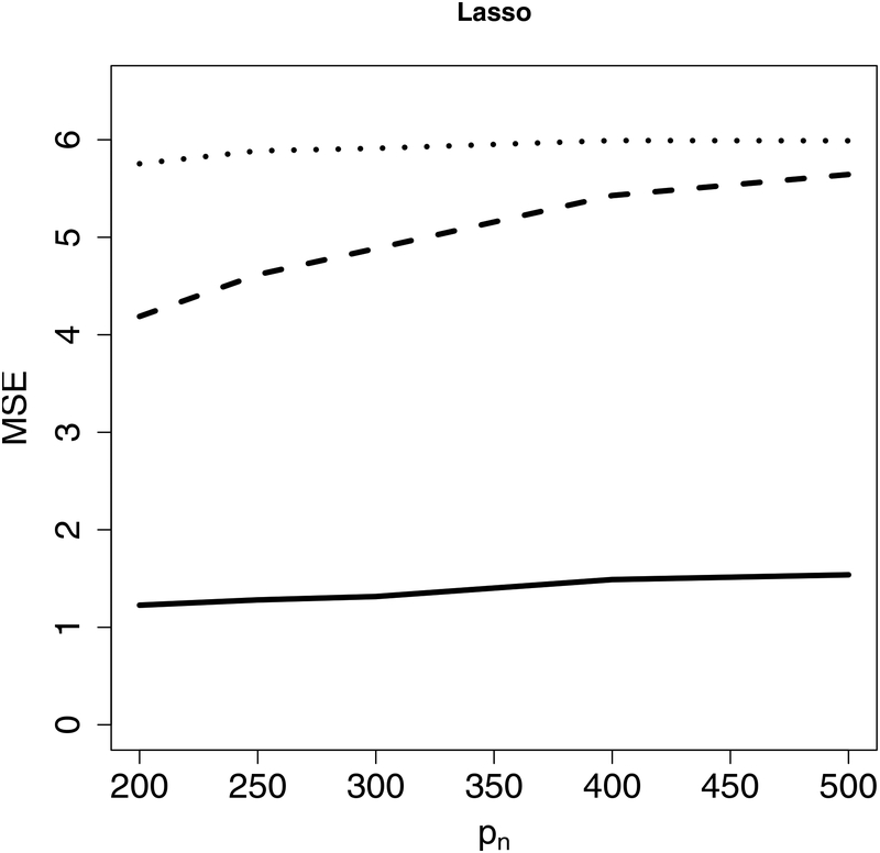
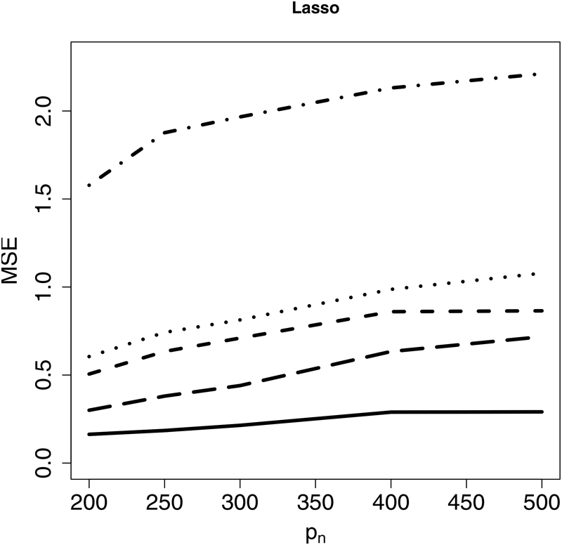
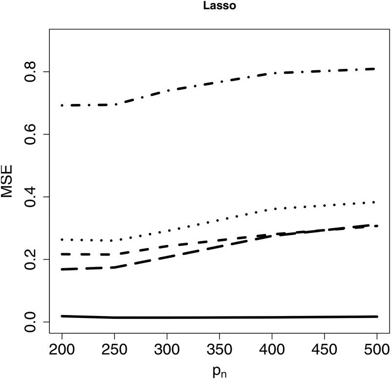
Next, we evaluate estimation accuracy on the targeted sub-model ${\mathcal{S}}_1\cup {\mathcal{S}}_{\text{WBC}}$ using the mean squared error (MSE) as the criterion under Examples 1–2. Figure 2 indicates that the proposed CIS-PSE detects WBC signals and provides more accurate and precise estimates. Figure 3 shows that CIS-PSE also improves the estimation of ${\beta }_{{\mathcal{S}}_1}$ Compared to PSE.

Figure 2:

The mean squared error (MSE) of ${\widehat{\beta }}_{{\mathcal{S}}_{\text{WBC}}}$ for different p’s under Example 1 (Left panel) and Example 2 (Right panel). Solid lines represent CIS-PSE, dashed lines are for PSE, and dotted lines indicate Lasso.

Figure 3:

The mean squared error (MSE) of ${\widehat{\beta }}_{{\mathcal{S}}_1}$ for different p’s under Example 1 (Left panel) and Example 2 (Right panel). Solid lines represent CIS-PSE, dashed lines are for PSE, dotted lines indicate Lasso RE defined as ${\widehat{\beta }}_{{\widehat{\mathcal{S}}}_1}^{\text{RE}}={\widehat{\Sigma }}_{{\widehat{\mathcal{S}}}_1}^{-1}\widehat{\text{ cov }}\left(x_{{\widehat{\mathcal{S}}}_1},y\right)$, dot-dashed lines represent Lasso, and long-dashed lines are for WR in (9).

We explore the prediction performanCe under Examples 1–2 using the mean squared prediction error (MSPE), defined as $\Vert \widehat{y}-y^{\text{test}}{\Vert }_2^2/n_{\text{test}}=\Vert X{\widehat{\beta }}^{\diamond }-y^{\text{test}}{\Vert }_2^2/n_{\text{test}}$, where ${\widehat{\beta }}^{\diamond }$ is obtained from the training data, y^test is the response variable for the test dataset, n_test is the size of test dataset, and ◊ represents either the proposed CIS-PSE or PSE. Table 2, whiCh summarizes the results, shows that CIS-PSE outperforms PSE, suggesting incorporating WBC signals helps to improve the prediction accuracy.

Table 2:

Mean squared prediction error (MSPE) of the predicted outcomes

	p	200	300	400	500
Example 1	CIS-PSE	3.17 (0.80)	3.19 (0.78)	3.25 (0.77)	3.32 (0.77)
	PSE	4.19 (0.83)	4.93 (1.02)	5.28 (1.07)	5.50 (1.16)
	Lasso	10.28 (5.68)	10.02 (5.58)	9.77 (4.96)	9.78 (4.54)
Example 2	CIS-PSE	0.65 (0.14)	0.92 (0.19)	1.30 (0.16)	2.43 (0.64)
	PSE	2.89 (0.61)	3.55 (0.75)	4.09 (0.68)	4.34 (0.97)
	Lasso	4.20 (0.79)	4.50 (0.88)	4.68 (0.90)	4.73 (0.97)

Lastly, we consider the setting where a subset of ${\mathcal{S}}_{\text{null}}$ is correlated with a subset of ${\mathcal{S}}_1$; see Example 3. Compared to Example 1, the results that are summarized in Table 4 show that the number of false positives only slightly increases, when some variables in ${\mathcal{S}}_{\text{null}}$ are correlated with variables in ${\mathcal{S}}_1$.

Table 4:

Estimation results of ${\mathcal{S}}_1$ and ${\mathcal{S}}_{\text{WBC}}$ from the growth rate data

When $\widehat{S_1}$ is selected by Lasso
$\widehat{S_1}$	${\widehat{\beta }}_{{\mathcal{S}}_1}^{\text{Lasso}}$	${\widehat{\beta }}_{{\mathcal{S}}_1}^{\text{PSE}}$	${\widehat{\beta }}_{{\mathcal{S}}_1}^{\text{CIS}-\text{PSE}}$	${\widehat{\mathcal{S}}}_{\text{WBC}}$	${\widehat{\beta }}_{{\mathcal{S}}_{\text{WBC}}}^{\text{CIS}-\text{PSE}}$	$\widehat{\text{corr}}$
TOT	0.06	2.85	3.73	-	-	-
LFERT	1.66	1.75	2.55	LLIFE	1.88	−.85
				NOM60	0.12	0.84
				NOF60	−0.10	0.83
				LGDPNOM60	−0.02	0.83
PRIF60	−0.001	−0.002	−0.12	LGDPPRIF60	0.02	0.99
				LGDPPRIM60	−0.02	0.93
				LGDPNOF60	0.02	−0.90
When $\widehat{S_1}$selected by adaptive Lasso
$\widehat{S_1}$	${\widehat{\beta }}_{{\mathcal{S}}_1}^{\text{ Ada-Lasso }}$	${\widehat{\beta }}_{{\mathcal{S}}_1}^{\text{PSE}}$	${\widehat{\beta }}_{{\mathcal{S}}_1}^{\text{CIS}-\text{PSE}}$	${\widehat{\mathcal{S}}}_{\text{WBC}}$	${\widehat{\beta }}_{{\mathcal{S}}_{\text{WBC}}}^{\text{CIS}-\text{PSE}}$	$\widehat{\text{corr}}$
LFERT	1.98	2.04	2.54	LLIFE	1.77	−0.85
				NOM60	0.08	0.84
				NOF60	−0.07	0.83
				LGDPNOM60	−0.01	0.83

^*$\widehat{\text{corr}}$ stands for the sample correlations between variables in $\widehat{{\mathcal{S}}_1}$ and ${\widehat{\mathcal{S}}}_{\text{WBC}}$.

^*TOT=The term of trade shock; LFERT=log of fertility rate (children per woman) averaged over 1960­1985; LLIFE=log of life expectancy at age 0 averaged over 1960–1985; NOM60=Percentage of no schooling in the male population in 1960; NOF60=Percentage of no schooling in the female population in 1960; LGDP60=log GDP per capita in 1960 (1985 price); PRIF60=Percentage of primary schooling attained in female population in 1960; PRIM60=Percentage of primary schooling attained in male population in 1960; LGDPNORM60=LGDP60×NOM60; LGDPPRIF60=LGDP60×PRIF60; LGDPPRIM60=LGDP60×PRIM60; LGDPNOF60=LGDP60×NOF60.

5. A real data example

We apply the proposed CIS-PSE method to analyze the gross domestic product (GDP) growth data studied in Gao et al. (2017) and Barro and Lee (1994). Our goal is to identify factors that are associated with the long-run GDP growth rate. The dataset includes the GDP growth rates and 45 socioeconomic variables for 82 countries from 1960 to 1985. We consider the following model:

$${\text{GR}}_i={\beta }_0+{\beta }_1\text{log}\left(\text{GDP}{60}_i\right)+z_i^{\text{T}}{\beta }_2+1\left(\text{GDP}{60}_i<2898\right)\left({\delta }_0+{\delta }_1\text{log}\left(\text{GDP}{60}_i\right)+z_i^{\text{T}}{\delta }_2\right)+{\epsilon }_i,$$ (16)

where i is the country indicator, i = 1, …, 82, GR_i is the annualized GDP growth rate of country i from 1960 to 1985, GDP60_i is the GDP per capita in 1960, and z_i are 45 socioeconomic covariates, the details of which can be found in Gao et al. (2017). The β₁ and β₂ represent the coefficients of log(GDP60) and socioeconomic predictors, respectively. The δ₀ represents the coefficient of whether the GDP per capita in 1960 is below a threshold (=2898) or not. The δ₁ represents the coefficient of log(GDP60) when GDP per capita in 1960 is below 2898. The δ₂ represent the coefficients of the interactions between the GDP60_i < 2898 and the socioeconomic predictors when GDP per capita in 1960 is below 2898.

We apply the proposed CIS-PSE and PSE by Gao et al. (2017) to detect ${\mathcal{S}}_1$. Additionally, CISPSE is used to further identify ${\mathcal{S}}_{\text{WBC}}$. Effects of covariates in ${\widehat{\mathcal{S}}}_1$ are estimated by Lasso, adaptive Lasso, PSE and CIS-PSE. Effects of covariates in ${\widehat{\mathcal{S}}}_{\text{WBC}}$ are estimated by CIS-PSE. The sample correlations between variables in ${\widehat{\mathcal{S}}}_1$ and ${\widehat{\mathcal{S}}}_{\text{WBC}}$ are also provided. Table 4 reports the selected variables and their estimated coefficients.

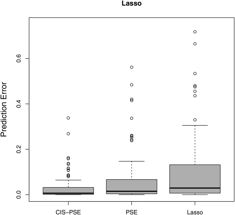
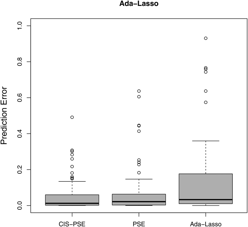
Next, we evaluate the accuracy of predicted GR using a leave-one-out cross-validation. For each country, we treat it itself as the test set while using all other countries as the training set. We apply Lasso, adaptive Lasso, PSE and CIS-PSE. All tuning parameters are selected as described in Section 4. The prediction results in Figure 4 show that CIS-PSE has the smallest prediction errors compared to PSE, Lasso and adaptive Lasso, with ${\widehat{\mathcal{S}}}_1$ detected by either Lasso or adaptive Lasso.

Figure 4:

Prediction errors from post-selection shrinkage estimators: CIS-PSE, PSE and two penalized estimators (Lasso and adaptive Lasso). $\widehat{{\mathcal{S}}_1}$ is detected by Lasso in the left panel and by adaptive Lasso in the right panel.

6. Discussion

To improve the estimation and prediction accuracy in high-dimensional linear regressions, we introduce the concept of weak but correlated (WBC) signals, which are commonly missed by the Lasso-type variable selection methods. We show that these variables can be easily detected with the help of their partial correlations with strong signals. We propose a CIS-PSE procedure for high-dimensional variable selection and estimation, particularly for WBC signal detection and estimation. We show that, by incorporating WBC signals, it significantly improves the estimation and prediction accuracy.

An alternative approach to weak signal detection would be to group them according to a known group structure and then select by their grouped effects (Bodmer and Bonilla, 2008; Li and Leal, 2008; Wu et al., 2011; Yuan and Lin, 2006). However, grouping strategies require prior knowledge on the group structure, and, in some situations, may not amplify the grouped effects of weak signals. For example, as pointed out in Buhlmann et al. (2013) and Shah and Samworth (2013), when a pair of highly negatively correlated variables are grouped together, they cancel out each other’s effect. On the other hand, our CIS-PSE method is based on detecting partial correlations and can accommodate the “canceling out” scenarios. Hence, when the grouping structure is known, it is worth combining the grouping strategy and CIS-PSE for weak signal detection. We will pursue this in the future.

Table 3:

Comparison of false positives (standard deviations in parentheses) between Examples 1 and 3

	p = 200	p = 300	p = 400	p = 500
Example 1	3.7 (2.4)	5.1 (2.7)	6.9 (3.1)	8.8 (3.3)
Example 3	4.6 (3.5)	6.1 (3.4)	7.8 (3.8)	10.9 (4.2)

7. Appendix

We provide technical proofs for Theorem 3.1, Corollary 3.2 and lemmas in this section. We first list some definitions and auxiliary lemmas.

Definition 7.1. A random vector Z = (Z₁, …, Z_p) is a sub-Gaussian with mean vector μ and variance proxy ${\sigma }_z^2$, if for any $a\in {ℝ}^p,E\left[\text{exp}\left\{a^{\text{T}}(Z-\mu )\right\}\right]\le \text{exp}\left({\sigma }_z^2\Vert a{\Vert }_2^2/2\right)$.

Let Z be a sub-Gaussian random variable with variance proxy ${\sigma }_z^2$. The sub-Gaussian tail inequality is given as, for any t > 0,

$$P(Z>t)\le e^{-\frac{t^2}{2{\sigma }_z^2}}\text{ and }P(Z<-t)\le e^{-\frac{t^2}{2{\sigma }_z^2}}.$$

The following Lemma 7.2 ensures that the set of signals with non-vanishing marginal sample correlations with y coincides with ${\mathcal{S}}_1$ with probability tending to 1. Therefore, evaluating condition (4) for a covariate j is equivalent to estimating nonzero Ω_jj’s for every $j^{\prime }\in S_1$. Let r_j′ be the rank of variable j′ according to the magnitude of $|\widehat{\text{ cov }}\left(X_{j^{\prime }},y\right)|,j^{\prime }=1,\dots ,p$. Denote by ${\tilde{\mathcal{S}}}_1(k)=\left\{j^{\prime }:r_{j^{\prime }}\le k\right\}$ the first k covariates with the largest absolute marginal correlations with y, for k = 1, …, p. Recall that $s_1=|{\mathcal{S}}_1|$.

Lemma 7.2. Under Assumption (A5), we have

$$\underset{n\to \infty }{\text{lim}}P\left({\tilde{\mathcal{S}}}_1\left(s_1\right)={\mathcal{S}}_1\right)=1.$$

Proof of Lemma 7.2. By the definition of ${\tilde{\mathcal{S}}}_1\left(s_1\right)$, it is suffice to show that with probability tending to 1, as n → ∞,

$$\text{max}\left|\frac{1}{n}{X}_{{\mathcal{S}}_1^{\text{c}}}^{\text{T}}y\right|<\text{min}\left|\frac{1}{n}{X}_{{\mathcal{S}}_1}^{\text{T}}y\right|.$$

Since $y=X{\beta }^{*}+\epsilon =X_{{\mathcal{S}}_0}{\beta }_{{\mathcal{S}}_0}^{*}+\epsilon =X_{{\mathcal{S}}_1}{\beta }_{{\mathcal{S}}_1}^{*}+X_{{\mathcal{S}}_2}{\beta }_{{\mathcal{S}}_2}^{*}+\mathit{\epsilon }$, we have

$$\frac{1}{n}{X}_{{\mathcal{S}}_1^c}^{\text{T}}y=\frac{1}{n}{X}_{{\mathcal{S}}_1^c}^{\text{T}}{X}_{{\mathcal{S}}_1}{\beta }_{{\mathcal{S}}_1}^{*}+\frac{1}{n}{X}_{{\mathcal{S}}_1^c}^{\text{T}}{X}_{{\mathcal{S}}_2}{\beta }_{{\mathcal{S}}_2}^{*}+\frac{1}{n}{X}_{{\mathcal{S}}_1^c}^{\text{T}}\epsilon .$$

Notice that for each $j^{\prime }\in {\mathcal{S}}_1^c,\frac{1}{n}{x}_{j^{\prime }}^{\text{T}}\epsilon \to \text{ cov }\left(X_{j^{\prime }},\epsilon \right)=0$ in probability, then $\text{max}|\frac{1}{n}{X}_{{\mathcal{S}}_1^c}^{\text{T}}\epsilon |=o_P(1)$ as n → ∞.

It follows that when n → ∞,

$$\text{max}\left|\frac{1}{n}{X}_{{\mathcal{S}}_1^{\text{c}}}^{\text{T}}y\right|\le \text{max}|{\Sigma }_{{\mathcal{S}}_1^c{\mathcal{S}}_1}{\beta }_{{\mathcal{S}}_1}^{*}|+\text{max}|{\Sigma }_{{\mathcal{S}}_1^c{\mathcal{S}}_2}{\beta }_{{\mathcal{S}}_2}^{*}|+o_P(1).$$

Similarly, when n → ∞,

$$\text{min}\left|\frac{1}{n}{X}_{{\mathcal{S}}_1}^{\text{T}}y\right|\ge \text{min}|{\Sigma }_{{\mathcal{S}}_1{\mathcal{S}}_1}{\beta }_{{\mathcal{S}}_1}^{*}|-\text{min}|{\Sigma }_{{\mathcal{S}}_1{\mathcal{S}}_2}{\beta }_{{\mathcal{S}}_2}^{*}|+o_P(1).$$

Lemma 7.2 is concluded by combining the above two inequalities with the faithfulness condition. ◻

Bickel and Levina (2008) showed that for $\alpha =O(\sqrt{\text{log}|{\mathcal{S}}_{[j]}|/n)},\Vert {\tilde{\Sigma }}_{[j]}^{\alpha }-{\Sigma }_{[j]}\Vert =O_P\left({\rho }_n\right)$, where ${\rho }_n=O\left(n^{-1}{C}_{\text{max}}^{1/4}\right)$ with $C_{\text{max}}^{1/4}$ given in (A6). Furthermore, Bickel and Levina (2008) and Fan et al. (2011) showed that the estimation error for each connected component of the precision matrix is bounded by

$$\Vert {\widehat{\mathbf{\Omega }}}_{[j]}-{\mathbf{\Omega }}_{[j]}\Vert =\Vert {\left({\tilde{\mathbf{\Sigma }}}_{[j]}^{\alpha }\right)}^{-1}-{\mathbf{\Sigma }}_{[j]}^{-1}\Vert =O_P\left({\rho }_n\right).$$ (17)

Here we adopt the recursive labeling Algorithm in Shapiro and Stockman (2002) to detect the connected components of the thresholded sample covariance matrix.

Without loss of generality, suppose that the strong signals in ${\widehat{\mathcal{S}}}_1$ belong to distinct connected components of ${\tilde{\Sigma }}^{\alpha }$. We rearrange the indices in ${\widehat{\mathcal{S}}}_1$ as $\left\{1,\dots ,|{\widehat{\mathcal{S}}}_1|\right\}$ and write the submatrix of ${\tilde{\Sigma }}^{\alpha }$ corresponding to $j^{\prime },1\le j^{\prime }\le |{\widehat{\mathcal{S}}}_1|$, as ${\tilde{\Sigma }}_{j^{\prime }}^{\alpha }$. For notational convenience, we rewrite

$$\widehat{\mathbf{\Omega }}=\text{diag}{\left({\left({\tilde{\mathbf{\Sigma }}}_1^{\alpha }\right)}^{-1},\dots ,{\left({\tilde{\mathbf{\Sigma }}}_{|{\widehat{\mathcal{S}}}_1^{(\alpha )}|}^{\alpha }\right)}^{-1},0\right)}_{p\times p}.$$

The following Lemma 7.3 is useful for controlling the size of ${\widehat{\mathcal{C}}}_{[j]}$.

Lemma 7.3. Under (A6)-(A7), when x is from a multivariate sub-Gaussian distribution, we have $P\left(|{\widehat{\mathcal{C}}}_{[j]}|\le O\left(n^{\xi }\right)\right)\ge 1-n^{\xi }{C}_1\text{exp}\left(-C_2{n}^{1+\xi }\right)$ for some positive constants C₁ and C₂.

Lemma 7.3 is a direct conclusion of Lemma 2.1 and Assumption (A6). Next we prove Theorem 3.1.

Proof of Theorem 3.1. Notice that ${\beta }_j^{*}={\sum }_{j^{\prime }\in {\mathcal{C}}_{[j]}}{\Omega }_{j{j}^{\prime }}\text{cov }\left(X_{j^{\prime }},y\right)$ and ${\widehat{\beta }}_j={\sum }_{j^{\prime }\in {\widehat{\mathcal{C}}}_{[j]}}{\widehat{\Omega }}_{j{j}^{\prime }}\widehat{\text{ cov }}\left(X_{j^{\prime }},y\right)$. Consider a sequence of thresholding parameters ν_n = O(n^3ξ/2) with a decreasing series of positive numbers u_n = 1 + n^−ξ/4 such that lim_n→∞ u_n = 1,

$$\begin{gathered} P\left(\left\{j\notin {\mathcal{S}}_1:|{\beta }_j^{*}|>{\nu }_n{u}_n\right\}\subseteq \left\{j\notin {\mathcal{S}}_1:|{\widehat{\beta }}_j|>{\nu }_n\right\}\right) \\ \ge 1-P\left(\underset{j\notin S_1,|{\beta }_j^{*}|>{\nu }_n{u}_n}{\cup }\left\{|{\widehat{\beta }}_j|\le {\nu }_n\right\}\right). \end{gathered}$$ (18)

Moreover, since $\left\{|{\widehat{\beta }}_j|\le {\nu }_n\right\}$ and $\left\{|{\beta }_j^{*}|>{\nu }_n{u}_n\right\}$, we have $|{\widehat{\beta }}_j-{\beta }_j^{*}|\ge {\nu }_n\left(u_n-1\right)$. As a result,

$$\begin{gathered} 1-P\left(\underset{j\notin S_1,|{\beta }_j^{*}|>{\nu }_n{u}_n}{\cup }\left\{|{\widehat{\beta }}_j|\le {\nu }_n\right\}\right) \\ \ge 1-\sum _{j\notin S_1,\left|{\beta }_j^{*}\right|>{\nu }_n{u}_n}P\left(|{\widehat{\beta }}_j-{\beta }_j^{*}|\ge {\nu }_n\left(u_n-1\right)\right). \end{gathered}$$ (19)

Notice that from Lemma 2.1, $P\left({\mathcal{C}}_{[j]}\subseteq {\widehat{\mathcal{C}}}_{[j]}\right)\ge 1-C_1{n}^{\xi }\text{exp}\left(-C_2{n}^{\xi }\right)$ for some positive constants C₁ and C₂ and 0 < ξ < 1. Therefore, we further have

$$\begin{gathered} P\left(\left|{\widehat{\beta }}_j-{\beta }_j^{*}\right|\ge {\nu }_n\left(u_n-1\right)\right) \\ =P\left(\left|\sum _{j^{\prime }\in {\mathcal{C}}_{\left[j\right]}}{\widehat{\Omega }}_{j{j}^{\prime }}\widehat{\text{ cov }}\left(X_{j^{\prime }},y\right)-\sum _{j^{\prime }\in {\mathcal{E}}_j}{\Omega }_{j{j}^{\prime }}\text{ cov }\left(X_{j^{\prime }},y\right)\right|\ge {\nu }_n\left(u_n-1\right)\right) \\ =P\left(\left|\sum _{j^{\prime }\in {\mathcal{C}}_{\left[j\right]}}{\widehat{\Omega }}_{j{j}^{\prime }}\widehat{\text{ cov }}\left(X_{j^{\prime }},y\right)-\sum _{j^{\prime }\in {\widehat{C}}_{\left[j\right]}}{\Omega }_{j{j}^{\prime }}\text{ cov }\left(X_{j^{\prime }},y\right)\right|\ge {\nu }_n\left(u_n-1\right)\right)+C_1{n}^{\xi }\text{exp}\left(-C_2{n}^{\xi }\right) \\ \le P\left(\sum _{j^{\prime }\in {\widehat{C}}_{\left[j\right]}}\left|\left({\widehat{\Omega }}_{j{j}^{\prime }}-{\Omega }_{j{j}^{\prime }}\right)\widehat{\text{ cov }}\left(X_{j^{\prime }},y\right)+{\Omega }_{j{j}^{\prime }}\left(\widehat{\text{ cov }}\left(X_{j^{\prime }},y\right)-\text{ cov }\left(X_{j^{\prime }},y\right)\right)\right|\ge {\nu }_n\left(u_n-1\right)\right)+C_1{n}^{\xi }\text{exp}\left(-C_2{n}^{\xi }\right) \\ \le P\left(\sum _{j^{\prime }\in {\widehat{\mathcal{C}}}_{\left[j\right]}}\left|\left({\widehat{\Omega }}_{j{j}^{\prime }}-{\Omega }_{j{j}^{\prime }}\right)\widehat{\text{ cov }}\left(X_{j^{\prime }},y\right)\right|\ge {\nu }_n\left(u_n-1\right)/2\right)+P\left(\sum _{j^{\prime }\in {\widehat{\mathcal{C}}}_{\left[j\right]}}\left|{\Omega }_{j{j}^{\prime }}\left(\widehat{\text{ cov }}\left(X_{j^{\prime }},y\right)-\text{ cov }\left(X_{j^{\prime }},y\right)\right)\right|\ge {\nu }_n\left(u_n-1\right)/2\right)+C_1{n}^{\xi }\text{exp}\left(-C_2{n}^{\xi }\right). \end{gathered}$$ (20)

By (17) and Assumption (A6), $\Vert \widehat{\Omega }-\Omega \Vert \le M{n}^{-(1-\xi /4)}$, for some 0 < M < ∞. As n → ∞, the first term in (20) can be shown as:

$$\begin{gathered} P\left(\sum _{j^{\prime }\in {\widehat{C}}_{[j]}}|\left({\widehat{\Omega }}_{j{j}^{\prime }}-{\Omega }_{j{j}^{\prime }}\right)\widehat{\text{ cov }}\left(X_{j^{\prime }},y\right)|>{\nu }_n\left(u_n-1\right)/2\right) \\ \le P\left(\frac{1}{n^2}{y}^{\text{T}}{x}_{\widehat{\mathcal{C}}[j]}{(\widehat{\mathbf{\Omega }}-\mathbf{\Omega })}_{j{\widehat{\mathcal{C}}}_{[j]}}^{\text{T}}{(\widehat{\mathbf{\Omega }}-\mathbf{\Omega })}_{j{\widehat{\mathcal{C}}}_{[j]}}{x}_{{\widehat{\mathcal{C}}}_{[j]}}^{\text{T}}y>\frac{{\nu }_n^2{\left(u_n-1\right)}^2}{4}\right) \\ \le P\left({\lambda }_{\text{max}}\left(\frac{1}{n}{x}_{{\widehat{C}}_{[j]}}{(\widehat{\mathbf{\Omega }}-\mathbf{\Omega })}_{j{\widehat{C}}_{[j]}}^{\text{T}}{(\widehat{\mathbf{\Omega }}-\mathbf{\Omega })}_{j{\widehat{\mathcal{C}}}_{[j]}}{x}_{{\widehat{\mathcal{C}}}_{[j]}}^{\text{T}}\right)\frac{1}{n}{y}^{\text{T}}y>\frac{{\nu }_n^2{\left(u_n-1\right)}^2}{4}\right). \\ \le P\left({\lambda }_{\text{max}}\left(\frac{1}{n}{x}_{{\widehat{\mathcal{C}}}_{[j]}}{x}_{{\widehat{\mathcal{C}}}_{[j]}}^{\text{T}}\right){\lambda }_{\text{max}}\left({(\widehat{\mathbf{\Omega }}-\mathbf{\Omega })}_{j{\widehat{\mathcal{C}}}_{[j]}}^{\text{T}}{(\widehat{\mathbf{\Omega }}-\mathbf{\Omega })}_{j{\widehat{C}}_{[j]}}\right)\frac{1}{n}{y}^{\text{T}}y>\frac{{\nu }_n^2{\left(u_n-1\right)}^2}{4}\right). \end{gathered}$$ (21)

Notice that $E\left[y^{\text{T}}y/n\right]=E\left(y^2\right)={\sigma }^2+{\left({\beta }^{*}\right)}^{\text{T}}\Sigma {\beta }^{*}\le {\sigma }^2+{\lambda }_{\text{max}}(\Sigma )\Vert {\beta }^{*}{\Vert }^2<{\tilde{C}}_1$ for some positive constant ${\tilde{C}}_1$. For sufficiently large n, ${\lambda }_{\text{max}}\left(x_{{\widehat{\mathcal{C}}}_{[j]}}{x}_{{\widehat{\mathcal{C}}}_{[j]}}^{\text{T}}/n\right)\le {\lambda }_{\text{max}}(\widehat{\Sigma })\le {\kappa }_2+{\lambda }_{\text{max}}(\widehat{\Sigma }-\Sigma )={\kappa }_2+\Vert \widehat{\Sigma }-\Sigma {\Vert }^{1/2}={\kappa }_2+O\left({\rho }_n^{1/2}\right)<{\tilde{C}}_2$ for some positive constant ${\tilde{C}}_2$. And ${\lambda }_{\text{max}}\left({(\widehat{\Omega }-\Omega )}_{j{\widehat{c}}_{[j]}}^{\text{T}}{(\widehat{\Omega }-\Omega )}_{j{\widehat{\mathcal{C}}}_{[j]}}\right)\le \Vert \widehat{\Omega }-\Omega {\Vert }^2\le M^2{n}^{-(2-\xi /2)}$ Therefore, from (21), for suffitiently large n,

$$\begin{gathered} P\left(\sum _{j^{\prime }\in {\widehat{\mathcal{C}}}_{[j]}}|\left({\widehat{\Omega }}_{j{j}^{\prime }}-{\Omega }_{j{j}^{\prime }}\right)\widehat{\text{ cov }}\left(X_{j^{\prime }},y\right)|>{\nu }_n\left(u_n-1\right)/2\right) \\ \le P\left({\tilde{C}}_2{M}^2\frac{1}{n}{y}^{\text{T}}y>n^{(2-\xi /2)}\frac{{\nu }_n^2{\left(u_n-1\right)}^2}{4}\right) \\ \le P\left(\frac{1}{n}{y}^{\text{T}}y>\frac{1}{{\tilde{C}}_2{M}^2}\frac{n^2}{4}\right)\le \frac{4{\tilde{C}}_2{M}^{2}E\left[y^{\text{T}}y/n\right]}{n^2}\le \frac{4{\tilde{C}}_1{\tilde{C}}_2{M}^2}{n^2}\to 0, \end{gathered}$$ (22)

where the second last step is from applying Markov inequality to the positively valued random variable y^Ty/n.

For the second term in (20), let $\tilde{z}={\left({\tilde{Z}}_1,\dots ,{\tilde{Z}}_p\right)}^{\text{T}}={\left({\text{x}}_1^{\text{T}}y/n-\text{ cov }\left(X_1,y\right),\dots ,{\text{x}}_p^{\text{T}}y/n-\text{cov }\left(X_p,y\right)\right)}^{\text{T}}$, then we have

$$\begin{gathered} P\left(\sum _{j^{\prime }\in {\widehat{C}}_{[j]}}|{\Omega }_{j{j}^{\prime }}\left(x_{j^{\prime }}^{\text{T}}y/n-\text{ cov }\left(X_{j^{\prime }},y\right)\right)|\ge {\nu }_n\left(u_n-1\right)/2\right) \\ \le P\left({\lambda }_{\text{max}}\left({\mathbf{\Omega }}^{\text{T}}\mathbf{\Omega }\right)\Vert {\tilde{z}}_{{\widehat{\mathcal{C}}}_{[j]}}{\Vert }_2^2\ge \frac{{\nu }_n^2{\left(u_n-1\right)}^2}{4}\right) \\ \le P\left(|{\tilde{Z}}_{j^{\prime }}|>\frac{{\nu }_n{\kappa }_1\left(u_n-1\right)}{2|{\widehat{C}}_{[j]}|}\right) \end{gathered}$$

for some $j^{\prime }\in {\widehat{\mathcal{C}}}_{[j]}$. Notice that $E\left[{\tilde{Z}}_{j^{\prime }}\right]=E\left[X_{j^{\prime }}y-\text{ cov }\left(X_{j^{\prime }},y\right)\right]=0$. Also $E\left[{\tilde{Z}}_{j^{\prime }}^2\right]=Var\left[X_{j^{\prime }}y\right]\le E\left[X_{j^{\prime }}^2{y}^2\right]\le \left(E\left(X_{j^{\prime }}^4\right)+E\left(y^4\right)\right)/2<{\tilde{C}}_3$ for some positive Constant ${\tilde{C}}_3$ as $E\left(X_{j^{\prime }}^4\right)\le {\lambda }_{\text{max}}^2(\Sigma )$ and $E\left(y^4\right)\le {\left({\lambda }_{\text{max}}(\Sigma )\Vert \beta {\Vert }^2\right)}^2+E\left({\epsilon }^4\right)<\infty$. Therefore, from Jensen’s inequality, $E\left[|{\tilde{Z}}_{j^{\prime }}|\right]=E\left[{\left({\tilde{Z}}_{j^{\prime }}^2\right)}^{1/2}\right]\le {\left(E\left[{\tilde{Z}}_{j^{\prime }}^2\right]\right)}^{1/2}\le {\tilde{C}}_3^{1/2}$. Then using Lemma 7.3 to Control the size of ${\widehat{C}}_{[j]}$ and applying Markov inequality on $|{\tilde{Z}}_{j^{\prime }}|$, we have

$$P\left(|{\tilde{Z}}_{j^{\prime }}|>\frac{{\nu }_n{\kappa }_1\left(u_n-1\right)}{2|{\widehat{\mathcal{C}}}_{[j]}|}\right)\le P\left(|{\tilde{Z}}_{j^{\prime }}|>\frac{{\kappa }_1{n}^{\xi /4}}{2}\right)\le \frac{2E\left[|{\tilde{Z}}_{j^{\prime }}|\right]}{{\kappa }_1{n}^{\xi /4}}\le \frac{2{\tilde{C}}_3^{1/2}}{{\kappa }_1{n}^{\xi /4}}\to 0.$$ (23)

Plugging (22) and (23) into (20) and then plugging (20) into (19) gives

$$\underset{n\to \infty }{\text{lim}}P\left(\left\{j\notin {\mathcal{S}}_1:|{\beta }_j^{*}|>{\nu }_n{u}_n\right\}\subseteq \left\{j\notin {\mathcal{S}}_1:|{\widehat{\beta }}_j|>{\nu }_n\right\}\right)=1.$$ (24)

By a similar argument, we also have

$$\underset{n\to \infty }{\text{lim}}P\left(\left\{j\notin {\mathcal{S}}_1:|{\beta }_j^{*}|>{\nu }_n/u_n\right\}\subseteq \left\{j\notin {\mathcal{S}}_1:|{\widehat{\beta }}_j|>{\nu }_n\right\}\right)=1.$$ (25)

Combining (24) and (25), we have

$$\underset{n\to \infty }{\text{lim}}P\left({\widehat{\mathcal{S}}}_{\text{WBC}}={\mathcal{S}}_{\text{WBC}}|{\widehat{\mathcal{S}}}_1={\mathcal{S}}_1\right).$$

◻

Proof of Corollary 3.2. Notice that

$$\begin{gathered} P\left(\left\{{\widehat{\mathcal{S}}}_{\text{WBC}}={\mathcal{S}}_{\text{WBC}}\right\}\cap \left\{{\widehat{\mathcal{S}}}_{2*}={\mathcal{S}}_{2*}\right\}\cap \left\{{\widehat{\mathcal{S}}}_1={\mathcal{S}}_1\right\}\right) \\ =P\left({\widehat{\mathcal{S}}}_{2*}={\mathcal{S}}_{2*}|\left\{{\widehat{\mathcal{S}}}_{\text{WBC}}={\mathcal{S}}_{\text{WBC}}\right\}\cap \left\{{\widehat{\mathcal{S}}}_1={\mathcal{S}}_1\right\}\right)P\left(\left\{{\widehat{\mathcal{S}}}_{\text{WBC}}={\mathcal{S}}_{\text{WBC}}\right\}\cap \left\{{\widehat{\mathcal{S}}}_1={\mathcal{S}}_1\right\}\right) \\ =P\left({\widehat{\mathcal{S}}}_{2*}={\mathcal{S}}_{2*}|{\widehat{\mathcal{S}}}_{1\text{WBC}}={\mathcal{S}}_{1\text{WBC}}\right)P\left({\widehat{\mathcal{S}}}_{\text{WBC}}={\mathcal{S}}_{\text{WBC}}|{\widehat{\mathcal{S}}}_1={\mathcal{S}}_1\right)P\left({\widehat{\mathcal{S}}}_1={\mathcal{S}}_1\right). \end{gathered}$$ (26)

Under the SRC in (A4), by Lemma 1 in Gao et al. (2017) or Theorem 2 in Zhang and Huang (2008),

$$\underset{n\to \infty }{\text{lim}}P\left({\widehat{\mathcal{S}}}_1={\mathcal{S}}_1\right)=1.$$ (27)

From Theorem 3.1,

$$\underset{n\to \infty }{\text{lim}}P\left({\widehat{\mathcal{S}}}_{\text{WBC}}={\mathcal{S}}_{\text{WBC}}|{\widehat{\mathcal{S}}}_1={\mathcal{S}}_1\right)=1.$$ (28)

Equations (27) and (28) together give ${\text{lim}}_{n\to \infty }P\left({\widehat{\mathcal{S}}}_{\text{WBC}}={\mathcal{S}}_{\text{WBC}}\right)=1$. This further gives that $P\left({\mathcal{S}}_1\subset {\widehat{\mathcal{S}}}_{1\text{WBC}}\subset \left\{{\mathcal{S}}_{1\text{WBC}}\cup {\mathcal{S}}_2\right\}\right)\to 1$. Then by Corollary 2 in Gao et al. (2017), we also have

$$\underset{n\to \infty }{\text{lim}}P\left(\left\{{\widehat{\mathcal{S}}}_{2*}={\mathcal{S}}_{2*}\right\}|\left\{{\widehat{\mathcal{S}}}_{1\text{WBC}}={\mathcal{S}}_{1\text{WBC}}\right\}\right)=1.$$ (29)

Combining (27), (28), (29) and (26) completes the proof. ◻

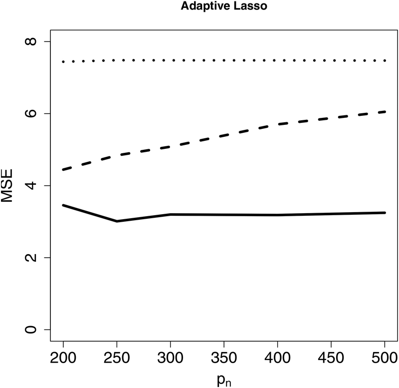
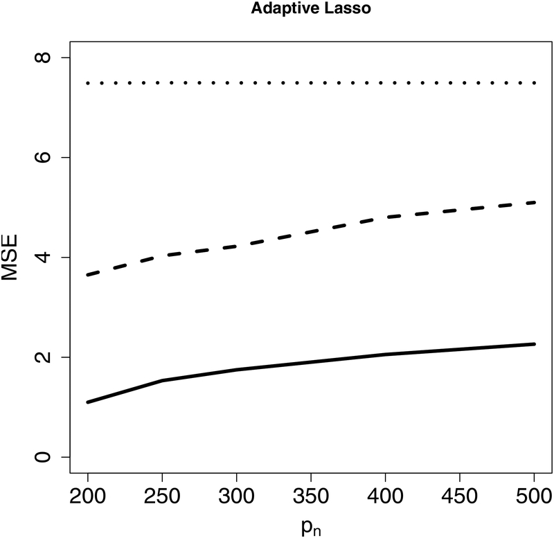
The following Tables 5–6 and Figures 5–6 give the selection, estimation and prediction results under Examples 1 and 2 when $\widehat{{\mathcal{S}}_1}$ is selected by adaptive Lasso.

Table 5:

The performance of variable selection on ${\mathcal{S}}_0$ when $\widehat{{\mathcal{S}}_1}$ is selected by adaptive Lasso

			p = 200	p = 300	p = 400	p = 500
Example 1	TP	CIS-PSE	61.4 (2.4)	61.1 (2.5)	61.0 (2.6)	61.1 (2.6)
		PSE	41.2 (5.0)	34.4 (5.1)	25.7 (6.1)	22.6 (5.8)
	FP	CIS-PSE	2.5 (2.1)	4.6 (2.5)	6.7 (3.2)	8.6 (3.0)
		PSE	15.1 (4.9)	19.7 (5.0)	22.3 (5.4)	28.0 (6.2)
Example 2	TP	CIS-PSE	62.5 (0.8)	58.0 (2.2)	54.6 (2.9)	52.0 (3.5)
		PSE	43.9 (3.8)	37 (4.2)	32.8 (4.3)	31.5 (4.2)
	FP	CIS-PSE	3.4 (2.6)	5.2 (3.0)	6.0 (3.5)	7.7 (4.1)
		PSE	13.1 (3.7)	18.6 (4.7)	21.9 (5.5)	28.0 (6.1)

Table 6:

Mean squared prediction error (MSPE) of the predicted outcomes when $\widehat{{\mathcal{S}}_1}$ is selected by adaptive Lasso

	p	200	300	400	500
Example 1	CIS-PSE	2.16 (0.57)	3.06 (0.63)	3.30 (0.72)	3.60 (0.81)
	PSE	3.91 (0.71)	4.85 (0.86)	5.71 (1.02)	6.27 (1.17)
	adaptive Lasso	15.02 (4.37)	14.67 (3.90)	14.49 (4.00)	14.74 (4.29)
Example 2	CIS-PSE	2.69 (0.58)	2.96 (0.72)	3.23 (0.81)	3.31 (0.83)
	PSE	3.77 (0.77)	4.76 (1.08)	5.50 (1.17)	5.82 (0.18)
	adaptive Lasso	4.48 (0.79)	4.81 (0.91)	4.94 (0.97)	4.97 (1.01)

Figure 5:

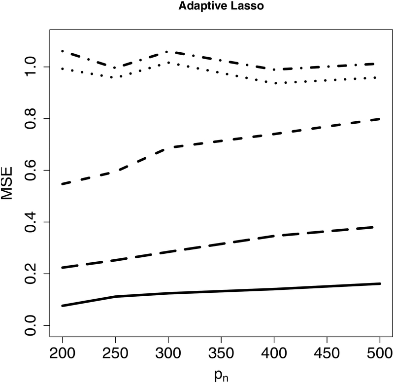
The mean squared error (MSE) of ${\widehat{\beta }}_{{\mathcal{S}}_{\text{WBC}}}$ for different p’s when $\widehat{{\mathcal{S}}_1}$ is selected by adaptive Lasso under Example 1 (Left panel) and Example 2 (Right panel). Solid lines represent CIS-PSE, dashed lines are for PSE, and dotted lines indicate adaptive Lasso.

Figure 6:

The mean squared error (MSE) of ${\widehat{\beta }}_{{\mathcal{S}}_1}$ for different p’s when $\widehat{{\mathcal{S}}_1}$ is selected by adaptive Lasso under Example 1 (Left panel) and Example 2 (Right panel). Solid lines represent CIS-PSE, dashed lines are for PSE, dotted lines indicate adaptive Lasso RE defined as ${\widehat{\beta }}_{{\widehat{\mathcal{S}}}_1}^{\text{RE}}={\widehat{\Sigma }}_{{\widehat{\mathcal{S}}}_1}^{-1}\widehat{\text{ cov }}\left(x_{{\widehat{\mathcal{S}}}_1},y\right)$ dot-dashed lines represent adaptive Lasso, and long-dashed lines are for WR in (9).

Figure 7 shows the averaged sum of squared prediction error (SSPE) on the validation datasets across 500 independent experiments for different α’s.

References

- Barro R and Lee J (1994). Data set for a panel of 139 countries. http://admin.nber.org/pub/barro.lee/.
- Bickel P and Levina E (2008). Covariance regularization by thresholding. Annals of Statistics, 36(6):2577–2604. [Google Scholar]
- Bodmer W and Bonilla C (2008). Common and rare variants in multifactorial susceptibility to common diseases. Nat. Genet, 40(6):695–701. [DOI] [PMC free article] [PubMed] [Google Scholar]
- Buhlmann P, Rütimann P, van de Geer S, and Zhang CH (2013). Correlated variables in regression: clustering and sparse estimation. Journal of Statistical Planning and Inference, 143:1835–1858. [Google Scholar]
- Fan J and Li R (2001). Variable selection via nonconcave penalized likelihood and its oracle properties. J. Am. Statist. Assoc, 96:1348–1360. [Google Scholar]
- Fan J, Liao Y, and Min M (2011). High-dimensional covariance matrix estimation in approxiamte factor models. Annals of Statistics, 39(6):3320–3356. [DOI] [PMC free article] [PubMed] [Google Scholar]
- Gao X, Ahmed SE, and Feng Y (2017). Post selection shrinkage estimation for highdimensional data analysis. Applied Stochastic Models in Business and Industry, 33(2):97–120. [Google Scholar]
- Li B and Leal S (2008). Methods for detecting associations with rare variants for common diseases: application to analysis of sequence data. Am. J. Hum. Genet, 83(3):311–321. [DOI] [PMC free article] [PubMed] [Google Scholar]
- Mazumder R and Hastie T (2012). Exact covariance thresholding into connected components for large-scale graphical lasso. Journal of Machine Learning Research, 12:723–736. [PMC free article] [PubMed] [Google Scholar]
- Shah RD and Samworth RJ (2013). Discussion of ‘correlated variables in regression: clustering and sparse estimation’. Journal of Statistical Planning and Inference, 143:1866–1868. [Google Scholar]
- Shao J, Wang Y, Deng X, and Wang S (2011). Sparse linear discriminant analysis by thresholding for high-dimensional data. Annals of Statistics, 39(2):1241–1265. [Google Scholar]
- Shapiro L and Stockman G (2002). Computer Vision. Prentice Hall. [Google Scholar]
- Tibshirani R (1996). Regression shrinkage and selection via the Lasso. J. R. Statist. Soc. B, 58:267–288. [Google Scholar]
- Wu MC, Lee S, Cai T, Li Y, Boehnke M, and Lin X (2011). Rare-variant association testing for sequencing data with the sequence kernel association test. Am J Hum Genet, 89(1):82–93. [DOI] [PMC free article] [PubMed] [Google Scholar]
- Yuan M and Lin Y (2006). Model selection and estimation in regression with grouped variables. J. R. Statist. Soc. B, 68:49–67. [Google Scholar]
- Zhang CH (2010). Nearly unbiased variable selection under minimax concave penalty. Annals of Statistics, 38(2):1567–1594. [Google Scholar]
- Zhang CH and Huang J (2008). The sparsity and bias of the LASSO selection in high dimensional linear regression. Annals of Statistics, 36:1567–1594. [Google Scholar]
- Zhang CH and Zhang S (2014). Confidence intervals for low dimensional parameters in high dimensional linear models. J. R. Statist. Soc. B, 76(1):217–242. [Google Scholar]
- Zou H (2006). The adaptive Lasso and its oracle properties. J. Am. Statist. Assoc, 101:1418–1429. [Google Scholar]