Does exclusion of extreme reporters of energy intake (the “Goldberg cutoffs”) reliably reduce or eliminate bias in nutrition studies? Analysis with illustrative associations of energy intake with health outcomes

ABSTRACT

Background

The Goldberg cutoffs are used to decrease bias in self-reported estimates of energy intake (EI_SR). Whether the cutoffs reduce and eliminate bias when used in regressions of health outcomes has not been assessed.

Objective

We examined whether applying the Goldberg cutoffs to data used in nutrition studies could reliably reduce or eliminate bias.

Methods

We used data from the Comprehensive Assessment of Long-Term Effects of Reducing Intake of Energy (CALERIE), the Interactive Diet and Activity Tracking in American Association of Retired Persons (IDATA) study, and the National Diet and Nutrition Survey (NDNS). Each data set included EI_SR, energy intake estimated from doubly labeled water (EI_DLW) as a reference method, and health outcomes including baseline anthropometric, biomarker, and behavioral measures and fitness test results. We conducted 3 linear regression analyses using EI_SR, a plausible EI_SR based on the Goldberg cutoffs (EI_G), and EI_DLW as an explanatory variable for each analysis. Regression coefficients were denoted , , and , respectively. Using the jackknife method, bias from compared with and remaining bias from compared with were estimated. Analyses were repeated using Pearson correlation coefficients.

Results

The analyses from CALERIE, IDATA, and NDNS included 218, 349, and 317 individuals, respectively. Using EI_G significantly decreased the bias only for a subset of those variables with significant bias: weight (56.1%; 95% CI: 28.5%, 83.7%) and waist circumference (WC) (59.8%; 95% CI: 33.2%, 86.5%) with CALERIE, weight (20.8%; 95% CI: −6.4%, 48.1%) and WC (17.3%; 95% CI: −20.8%, 55.4%) with IDATA, and WC (−9.5%; 95% CI: −72.2%, 53.1%) with NDNS. Furthermore, bias significantly remained even after excluding implausible data for various outcomes. Results obtained with Pearson correlation coefficient analyses were qualitatively consistent.

Conclusions

Some associations between EI_G and outcomes remained biased compared with associations between EI_DLW and outcomes. Use of the Goldberg cutoffs was not a reliable method for eliminating bias.

Introduction

The study of energy intake (EI) is of vital interest in nutrition and obesity research. Methods to measure EI in units of metabolizable energy are roughly divided into calculation from energy balance [respiratory gas analysis or doubly labeled water (DLW)], self-reporting, and direct observation (not discussed herein). Because respiratory gas analysis necessitates substantial behavioral restriction on the subjects, DLW is widely accepted as a reference method for measuring total energy expenditure (TEE) and EI in free-living humans (1–3). However, it “is often not practical given the high costs of isotopes and equipment for isotope analysis, as well as the expertise required for analysis” (4). The second method is self-reported estimates of EI (EI_SR), in which calorie intake is calculated from foods and beverages consumed during the study period by using food diaries or FFQs (5–7). EI_SR was the primary method used to calculate EI before the more sophisticated methods, including respiratory gas analysis and DLW, were developed. However, it is now well known that self-reports are severely error prone and usually underestimate (but sometimes overestimate) actual EI (8), and the use of EI_SR is widely discouraged (9).

To mitigate the error in EI_SR, excluding implausible (over- and/or under-) reporters before analyses is sometimes suggested (4). The most commonly used method is to apply a cutoff rule to identify implausible reporters. Among the various cutoff rules, rules incorporating EI_SR adjusted by predicted TEE (and the measurement errors) have been proposed to address individual variance. Methods to estimate TEE vary substantially. For example, Goldberg et al. (10) proposed using TEE estimated as a product of basal metabolic rate (BMR) and physical activity level (PAL). Herein, we refer specifically to the original process proposed by Goldberg et al. (10) as “using the Goldberg cutoffs”; after biologically implausible reporters of EI are removed from the data, the remaining data are denoted EI_G.

Especially in situations where DLW cannot be used, EI_G is still used to investigate associations between EI and health outcomes, which implicitly suggests that those investigators believe that application of the cutoff rules will render less-biased results or results without bias. Given that the Goldberg cutoffs exclude only extreme reporters, but not mildly inaccurate reporters, whether use of the cutoff rules actually reduces bias is not obvious. This question has not been evaluated in empirical studies and no formal theoretical foundation (i.e., mathematical proof) for claiming that it does actually reduce bias has been shown. In this study, we applied the Goldberg cutoffs to evaluate the reliability of these rules in eliminating or reducing bias in nutrition and obesity studies through the analysis of 3 independent data sources. We hypothesized that the Goldberg cutoffs would reduce the bias to some extent but that some bias would remain.

Methods

The predetermined study purpose and analytical approach were to assess the bias due to EI_SR, and to evaluate bias reduction from using the Goldberg cutoffs, by comparing regression coefficients using the estimated EIs. The choice of which health and behavioral outcomes to evaluate was determined upon viewing the data dictionaries of the 3 data sets used, and selecting outcomes that have been postulated to be related to EI. The parameters used for calculating Goldberg cutoffs are described in the Supplemental Methods. All Goldberg parameters and outcomes that we analyzed are presented herein.

Data sources

We used 3 data sources for the purpose of comparison and validation: Comprehensive Assessment of Long-Term Effects of Reducing Intake of Energy (CALERIE) Phase 2, the Interactive Diet and Activity Tracking in American Association of Retired Persons (IDATA) study, and the National Diet and Nutrition Survey (NDNS). The first 2 data sources are from the United States and the third is from the United Kingdom. For each data source, we extracted data including 1) EI_SR and EI estimated from DLW (which we named EI_DLW) and 2) health outcomes for each participant. Various health outcomes were available for each data source; however, we selected several variables for our analyses that were 1) potentially associated with EI, 2) objective physical measurements (including biomarkers) or behavioral measurements, and 3) measured in the same month that EI_SR and EI_DLW were measured. All variables we analyzed are reported herein. We used multiple data sources and a wide range of the measured health outcomes to assess the extent of generalizability of the results (i.e., different populations and different outcomes) and to broadly understand the magnitude of improvement in the estimation of associations between EI and health outcomes by applying the Goldberg cutoffs. These 3 data sources were specifically selected because they have the necessary information for this study and because the subset of individuals included from these studies were not part of an intervention program (such as a weight loss intervention), given that EI_DLW is known to be biased under energy imbalance (11). The details of the measurement process, schedule of EI estimation, and health outcomes are available in the Supplemental Methods. The following sample sizes were used in the analyses: 218 for CALERIE, 349 for IDATA, and 371 for NDNS (see Supplemental Figure 1). CALERIE data were freely available through the study website: https://calerie.duke.edu/ (downloaded 5 September, 2018). IDATA data were accessible through the Cancer Data Access System (https://biometry.nci.nih.gov/cdas/idata/; downloaded 22 November, 2017) after our project proposal was reviewed and approved by the National Cancer Institute (https://biometry.nci.nih.gov/cdas/approved-projects/1702/). NDNS data were available through the UK Data Archive (https://www.ukdataservice.ac.uk/; downloaded 20 June, 2018) after the review and approval of our project proposal (Project ID: 123982).

The Goldberg cutoffs

The Goldberg cutoffs refer to a method originally introduced by Goldberg et al. (10) to exclude individuals who report unrealistically high or low EI. In the process of the Goldberg cutoffs, the ratio of EI_SR to TEE estimated from body composition and PAL is calculated for each individual. Individuals who fall outside the following range are classified as underreporters or overreporters and are excluded from subsequent analyses:

(1)

where S is defined as

(2)

and is the within-subject CV in EI_SR, is the within-subject CV in BMR, is the total variation in PAL, and d is the number of days of diet assessment. TEE is assumed to be a product of BMR and PAL. PAL is set as 1.75 (1.79 for men and 1.72 for women) for the average industrialized nation per the review article by Dugas et al. (12) and is the value we used herein. BMR is estimated from the equation proposed by Cunningham (13):

(3)

where FFM means fat-free mass. Only the mean of daily EI_SR is available for each data set; there are no repeated measurements of BMR (or body composition) and PAL is assumed (fixed), so we set , , , and , as was suggested in a previous study (14).

Statistical analysis

To assess the bias due to self-report and the reduction in bias by use of the Goldberg cutoffs, we conducted 3 linear regression analyses separately. In all analyses, the aforementioned health-related outcomes were used as dependent variables and EI was used as an independent variable. For some of the variables, energy balance (i.e., EI − TEE) might be a better independent variable than EI. Furthermore, important covariates might be missed. However, we focused on crude associations between EI and health outcomes because 1) the purpose of this study was not causal inference about the relations between these variables per se and 2) we wanted to comprehensively evaluate the ability of the Goldberg cutoffs to reduce bias across different types of outcomes.

The first analysis used EI_SR as an independent variable. The second analysis removed the reporters with implausible EI_SR by using the Goldberg cutoffs (the remaining data were denoted as EI_G). The third analysis used EI_DLW as an independent variable. The estimated linear regression coefficients from each model are described as , , and , respectively. To assess whether the bias due to self-reporting was significant, we defined and computed percentage bias () of the estimated linear regression coefficient:

(4)

Percentage bias is interpreted as (see Figure 1 for a graphical representation):

1. no bias (; ),

2. overestimation (),

3. underestimation ().

FIGURE 1.

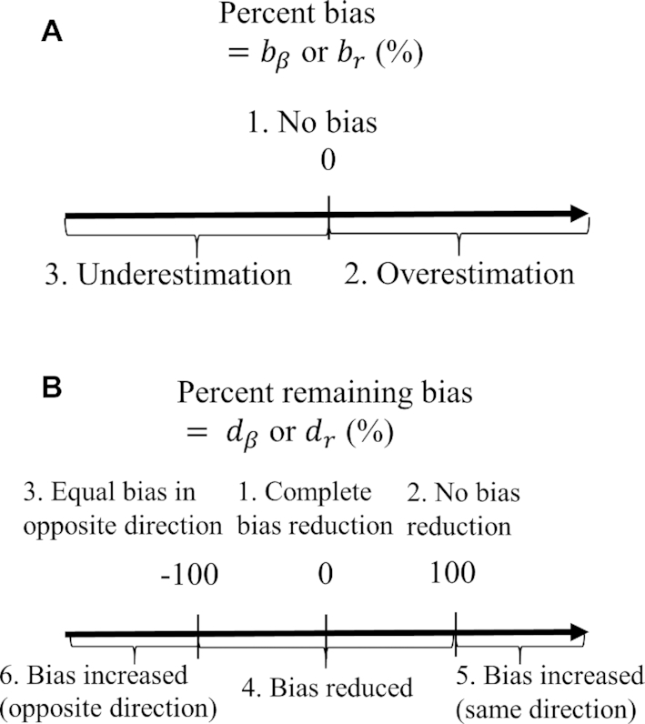
Interpretation of percentage bias and percentage remaining bias. (A) Graphical interpretation of percentage bias. In the case of no bias, the estimated coefficients using self-reported EI as an independent variable are equal to those using EI estimated from DLW. (B) Graphical interpretation for percentage remaining bias. Percentage remaining bias determines whether the Goldberg cutoffs significantly reduce the bias due to self-reporting. The narrative interpretation of each case is available in the main text. , percentage bias in the estimated linear regression coefficient; , percentage bias in the Pearson correlation coefficient; , percentage remaining bias in the estimated linear regression coefficient; , percentage remaining bias in the Pearson correlation coefficient; DLW, doubly labeled water; EI, energy intake.

Furthermore, to test whether the Goldberg cutoffs significantly eliminated or reduced the bias due to self-reporting, we defined and computed percentage remaining bias () in the estimated regression coefficients after applying the Goldberg cutoffs (removing implausible EI_SR):

(5)

To illustrate the interpretation of , consider the point estimates of using body weight as an outcome for CALERIE: 7.39, 9.88, and 13.07, respectively (see Results). In this example, the estimated coefficient after applying the Goldberg cutoffs (= 9.88) was still different than the “true” coefficient (= 13.07): . The nonzero value of the difference suggests that bias remains. However, this quantity by itself does not tell us whether and by how much the bias is reduced (or increased) compared with the uncorrected self-report. For this purpose, we can use the bias before applying the Goldberg cutoffs as a reference: . The quotient of these 2 values () quantifies the remaining bias relative to the original bias. In other words, 43.9% of the original bias was reduced by the Goldberg cutoffs, but it is not a perfect reduction ( is not zero).

Following are the more nuanced interpretations of percentage remaining bias (see Figure 1 for a graphical representation):

1. Complete bias reduction (bias elimination) (; )

2. No bias reduction (; )

3. Equal bias in opposite direction (; )

4. Bias reduced to some extent (; )

5. Bias increased in the same direction ()

6. Bias increased in the opposite direction ()

For clarity, if is in the range −100 to 100, it implies bias was reduced to some extent. If is 0, it implies complete bias reduction (or bias elimination). We then used jackknife estimation (leave one out) (15) to construct 95% CIs of the results (see the Supplemental Methods for details of the computational processes). These analyses were executed separately for each outcome.

Pearson correlation coefficients are also frequently used to examine the associations between EI and health outcomes. Because Pearson correlation coefficients are unitless quantities of linear associations, it is useful to compare the difference in associations between different outcomes (with different units). Hence, we also performed the same analysis for the Pearson correlation coefficient (r): , , for which the in Equations 4 and  5 are simply replaced by r and the interpretation of bias and remaining bias follows logically.

A 2-tailed Student t test was used to test whether bias was significantly different from 0. A 2-tailed independent Welch t test was used to test the mean difference in bias between the accepted and rejected cases within each data set. The jackknife method was used to test the mean difference in bias between the accepted and the whole cases within each data set. The 95% CIs were computed based on the estimated variance of the jackknife estimator. As a sensitivity analysis, we also computed empirical 95% CIs using inflated jackknife values to account for potential nonnormality (see the Supplemental Methods). The type I error rate was fixed at 0.05 (2-tailed). All analyses were performed with the statistical computing software R (The R Foundation for Statistical Computing) version 3.4.1.   Table 1 summarizes the parameters and the variables used.

TABLE 1.

Model parameters and variables

Variables and parameters	Description
EISR	Self-reported estimates of energy intake
EIG	Self-reported energy intake after excluding implausible EISR using the Goldberg cutoffs
EIDLW	Energy intake estimated using doubly labeled water
	Estimated coefficients using EISR as an independent variable
	Estimated coefficients using EIG as an independent variable
	Estimated coefficients using EIDLW as an independent variable
	Pearson correlation coefficient between EISR and health outcomes
	Pearson correlation coefficient between EIG and health outcomes
	Pearson correlation coefficient between EIDLW and health outcomes
	Percentage bias in the estimated linear regression coefficient
	Percentage remaining bias in the estimated linear regression coefficient
	Percentage bias in the Pearson correlation coefficient
	Percentage remaining bias in the Pearson correlation coefficient

Results

Overview of the data

Table 2 shows the descriptive statistics for each data source. The Goldberg cutoffs resulted in 17.0% (n = 37), 50.7% (n = 177), and 25.7% (n = 96) of subjects being excluded from the analysis of the CALERIE, IDATA, and NDNS data sets, respectively. In each data set, significant underreporting was observed among both the rejected and the accepted cases, although the magnitude of underreporting was significantly smaller among the accepted cases than among the rejected ones. This suggests that the Goldberg cutoffs exclude extreme cases of underreporting but do not exclude mild cases.

TABLE 2.

Baseline characteristics of individuals included in the data analyses¹

Variable	CALERIE	IDATA	NDNS
n	218	349	371
Excluded by the Goldberg cutoffs	37 (17.0)	177 (50.7)	96 (25.9)
Age, y	38.1 ± 7.2	63.0 ± 6.0	34.7 ± 25.6
Male	66 (30.3)	148 (42.4)	183 (49.3)
Race
Non-Hispanic white	166 (76.1)	325 (93.1)	344 (92.7)
African American	27 (12.4)	22 (6.3)	4 (1.1)
Other	25 (11.5)	2 (0.6)	23 (6.2)
Weight, kg	71.8 ± 9.2	79.8 ± 17.0	62.8 ± 25.3
Height, cm	168.7 ± 8.5	169.2 ± 9.3	157.4 ± 19.4
Waist circumference, cm	80.8 ± 7.6	92.2 ± 14.1	90.0 ± 16.0
BMI, kg/m2	25.1 ± 1.7	27.7 ± 4.7	24.2 ± 6.5
Fat-free mass, kg	48.2 ± 9.0	49.3 ± 10.9	41.2 ± 14.8
Daily EI estimated from food diary (EISR), kcal/d	2101 ± 532	1780 ± 761	1798 ± 466
Daily EI estimated from DLW (EIDLW), kcal/d	2412 ± 442	2419 ± 516	2517 ± 682
Reporting bias, EISR − EIDLW	−311 ± 4462, 3	−639 ± 7732, 3	−719 ± 5902, 3
Reporting bias among accepted cases,4 EISR − EIDLW	−220 ± 3992, 3, 5	−228 ± 4772, 3, 5	−557 ± 4832, 3, 5
Reporting bias among rejected cases,6 EISR − EIDLW	−758 ± 3972, 5	−1039 ± 7972, 5	−1186 ± 6242, 5

¹Values are mean ± SD or n (%) unless otherwise indicated. CALERIE, Comprehensive Assessment of Long-Term Effects of Reducing Intake of Energy; EI_DLW, energy intake estimated using doubly labeled water; EI_G, self-reported energy intake after excluding implausible EI_SR using the Goldberg cutoffs; EI_SR, self-reported estimates of energy intake; IDATA, Interactive Diet and Activity Tracking in American Association of Retired Persons; NDNS, National Diet and Nutrition Survey.

²The reporting bias is significant (P < 0.05; 2-tailed Student t test).

³Significant difference between the accepted cases and the rejected cases within each data set (P < 0.05; jackknife method).

⁴The individuals who were considered to be plausible by the Goldberg cutoffs.

⁵Significant difference between the accepted cases (cases remaining after implementation of the Goldberg cutoffs) and the rejected cases (cases excluded after implementation of the Goldberg cutoffs) within each data set (P < 0.05; 2-tailed independent Welch t test).

⁶The individuals who were considered to be implausible by the Goldberg cutoffs.

The 3 data sources differed in terms of some population characteristics. For example, the participants in IDATA were the heaviest and had the highest waist circumference (WC) and BMI. The participants in IDATA were older than those in the other data sources and the proportion of male participants was higher in NDNS than in CALERIE. Among the 3 data sets, daily EI_SR was highest in the CALERIE data set; the CALERIE reporting bias in EI was also the smallest.

Associations between DLW and health outcomes

Supplemental Figures 2 and 3 show the best-fit lines from the 3 regression models along with the data for EI_SR and EI_DLW for the 3 data sources. In most cases, the slope of the line estimated from EI_G (dotted green line, ) was closer to the slope of the line estimated from EI_DLW (solid blue line, ) than that estimated from EI_SR (dashed red line, ), which suggests that the Goldberg cutoffs mitigate bias in the association estimate caused by self-report. The analysis using EI_DLW () revealed that EI was significantly associated with weight, WC, systolic blood pressure (SBP), LDL, HDL, and leptin in CALERIE; with weight, WC, SBP, and diastolic blood pressure (DBP) in IDATA; and with weight, WC, SBP, DBP, and HDL in NDNS (Supplemental Table 1). It is worth noting that the associations between EI_DLW and weight, WC, and SBP, which were measured in all 3 studies, were consistently significant, although the estimated values were not numerically consistent between the data sources.

Bias estimation comparing EI_SR with EI_DLW

To test whether was significantly different from , we computed percentage bias: (Supplemental Table 1 and the left panel in Figure 2). Significant underestimation was observed for weight, WC, SBP, DBP, and LDL in CALERIE; for weight, WC, SBP, and DBP in IDATA; and for weight, WC, and SBP in NDNS. Among them, the largest magnitude percentage bias was −150.7% (95% CI: −272.4%, −28.9%) for DBP in CALERIE. No significant overestimation was observed for any outcomes.

FIGURE 2.

Percentage bias and percentage remaining bias of the estimated linear regression coefficient. Italic bold font means significant association between EI_DLW and the outcome. (Left panel) Percentage bias of the estimated linear regression coefficient, , was computed. The open point symbols (squares: CALERIE; circles: IDATA; and triangles: NDNS) correspond to the maximum likelihood estimators (MLEs) and the bars are 95% CIs. When the MLEs are <−200 or >200, the filled symbols are plotted at the left end or right end of the panel. The 95% CIs were computed using parametric assumptions about the distribution of jackknife estimators. *Significant bias was observed. (Right panel) Percentage remaining bias of the estimated linear regression coefficient, , was computed. ^#Significant bias reduction was observed (i.e., the 95% CI of percentage remaining bias is within −100 to 100). ^$Significant remaining bias was observed (i.e., the 95% CI of remaining bias does not exclude 0). , percentage bias in the estimated linear regression coefficient; CALERIE, Comprehensive Assessment of Long-Term Effects of Reducing Intake of Energy; DBP, diastolic blood pressure; , percentage remaining bias in the estimated linear regression coefficient; EI_DLW, energy intake estimated from doubly labeled water; EI_G, plausible self-reported estimates of energy intake based on the Goldberg cutoffs; EI_SR, self-reported estimates of energy intake; HR, heart rate; IDATA, Interactive Diet and Activity Tracking in American Association of Retired Persons; NDNS, National Diet and Nutrition Survey; PSQI, Pittsburgh Sleep Quality Index; SBP, systolic blood pressure; VO₂ max, maximal oxygen consumption; , estimated coefficient using EI_DLW as an independent variable; , estimated coefficient using EI_G as an independent variable; , estimated coefficient using EI_SR as an independent variable.

Remaining bias with EI_G

After applying the Goldberg cutoffs and excluding data with implausible EI_SR, biases were expected to be eliminated, or reduced to some extent. To test this, we computed percentage remaining bias: (Supplemental Table 1 and the right panel in Figure 2). Among the outcomes with significant bias, significant bias reduction (i.e., the 95% CI for percentage remaining bias was in the range −100 to 100) was observed only for weight (56.1%; 95% CI: 28.5%, 83.7%) and WC (59.8%; 95% CI: 33.2%, 86.5%) with CALERIE; for weight (20.8%; 95% CI: −6.4%, 48.1%) and WC (17.3%; 95% CI: −20.8%, 55.4%) with IDATA; and for WC (−9.5%; 95% CI: −72.2%, 53.1%) with NDNS. We did not observe significant bias increase for any outcome in the analyses. Among the outcomes with significant bias, significant remaining bias (i.e., the 95% CI for percentage remaining bias excluded 0) was observed for weight, WC, SBP, DBP, and LDL in the CALERIE data set; and for SBP in the IDATA data set, meaning we cannot always expect perfect bias correction (i.e., bias elimination). We used Pearson correlation coefficients alternatively to the regression coefficients, and the results were qualitatively consistent with those for regression coefficients (Supplemental Table 2 and Figure 3). Our sensitivity analysis using empirical 95% CIs from inflated jackknife values resulted in qualitatively similar results (Supplemental Figures 4 and 5, Supplemental Tables 3 and 4).

FIGURE 3.

Percentage bias and percentage remaining bias of the Pearson correlation coefficient. Italic bold font means significant association between EI_DLW and the outcome. (Left panel) Percentage bias of the Pearson correlation coefficient, , was computed. The open point symbols (squares: CALERIE; circles: IDATA; and triangles: NDNS) correspond to the maximum likelihood estimators (MLEs) and the bars are 95% CIs. When the MLEs are <−200 or >200, the filled symbols are plotted at the left end or right end of the panel. The 95% CIs were computed using parametric assumptions about the distribution of jackknife estimators. *Significant bias was observed. (Right panel) Percentage remaining bias of the Pearson correlation coefficient, , was computed. ^#Significant bias reduction was observed (i.e., the 95% CI of percentage remaining bias is within −100 to 100). ^$Significant remaining bias was observed (i.e., the 95% CI of remaining bias does not exclude 0). Model parameters and variables are defined in Table 1. , percentage bias in the Pearson correlation coefficient; CALERIE, Comprehensive Assessment of Long-Term Effects of Reducing Intake of Energy; DBP, diastolic blood pressure; , percentage remaining bias in the Pearson correlation coefficient; EI_DLW, energy intake estimated from doubly labeled water; EI_G, plausible self-reported estimates of energy intake based on the Goldberg cutoffs; EI_SR, self-reported estimates of energy intake; HR, heart rate; IDATA, Interactive Diet and Activity Tracking in American Association of Retired Persons; NDNS, National Diet and Nutrition Survey; PSQI, Pittsburgh Sleep Quality Index; , Pearson correlation coefficient between EI_DLW and health outcomes; , Pearson correlation coefficient between EI_G and health outcomes; , Pearson correlation coefficient between EI_SR and health outcomes; SBP, systolic blood pressure; VO₂ max, maximal oxygen consumption.

In summary, the Goldberg cutoffs failed to consistently demonstrate statistically significant bias reduction, with some, but not all, cases demonstrating statistically significant bias reduction. Furthermore, in some cases, the Goldberg cutoffs did not eliminate the bias (i.e., bias remained after applying the Goldberg cutoffs), as evidenced by the CIs ruling out complete bias reduction.

Discussion

The mechanism of the bias in EI_SR has been discussed for ≥60 y (16). Heymsfield et al. (17) further pointed out other reasons, such as psychosocial motivation (social desirability) and inaccurate food labeling.

The Goldberg cutoffs were proposed to address this issue, and have been used in various nutrition studies to exclude implausible EI_SR (18–22). Furthermore, the Goldberg cutoffs have also been used as a process to exclude implausible dietary data more generally (23–27). The rationality of using the Goldberg cutoffs to exclude implausible dietary data is based on an implicit assumption: “if total EI is underestimated, it is probable that the intakes of other nutrients are also underestimated” (28).

In this study, we examined whether applying the Goldberg cutoffs reduces or eliminates the bias in the estimated associations between outcomes and EI_SR using EI_DLW as the reference method. Significant bias and bias reduction in the associations between EI_SR and health outcomes using the Goldberg cutoffs (EI_G) were observed only for some outcomes. Furthermore, we rejected the hypothesis that bias was perfectly eliminated in many cases. Although quantitatively inconsistent, we could confirm qualitatively similar results for the same outcomes across data sources in which the characteristics of the populations differ. Our findings collectively suggest that the degree of bias and bias reduction is dependent on population characteristics and health outcomes.

We observed substantial differences in population characteristics between the different sources: age, sex, and race structure. This might have resulted in the quantitative differences in the results. Regarding the proportion of the excluded population, it varied between the 3 data sources; however, the proportions for CALERIE and NDNS were comparable with a previous study using NHANES data (18% for men and 28% for women) (29). The proportion of the excluded population for IDATA (50.7%) is higher than for the other 2. One possible reason is that we used the EI_SR estimate based on FFQs, for which the magnitude of underreporting is known to be higher than for other methods such as food diary and food record (30).

The strengths of our approach are 4-fold. First, EI_SR and EI_DLW were obtained from the same individuals. McCrory et al. (31) and Huang et al. (32) addressed similar questions, but the data for EI_SR and the data for EI_DLW were independent. Given that the estimated associations between EI_DLW and health outcomes differed between the data sources (see Supplemental Table 1 and Figure 2), it is necessary to use EI_SR and EI_DLW data measured in the same individuals for our study purpose. Second, we used multiple health outcomes to more thoroughly understand the utility of the Goldberg cutoffs, although some previous literature [Huang et al. (32) and McCrory et al. (31)] used only body weight. Third, we quantitatively assessed and tested the bias and bias reduction in the estimation of the association induced by the Goldberg cutoffs by the jackknife method. The previous studies simply listed the estimated coefficients (i.e., , and ) in parallel, and assessed the difference by comparing the values without a formal test (31–34). Fourth, we used multiple health outcomes as dependent variables, which strengthened the generalizability of our results across outcomes.

These analyses do have limitations. The major limitation is that the findings are just associations and are not designed to yield causal relations. Furthermore, the estimated associations were not adjusted by potential confounders, and adding confounding variables in the analyses might alter estimates of bias and bias reduction. Moreover, some of the underlying relations may be more strongly associated with energy balance (e.g., EI – energy expenditure) rather than EI alone. However, even when energy expenditure is known, it is not a measure of energy balance, and bias in EI_SR, even when applying the Goldberg cutoffs, likely influences the accuracy and precision of a calculated energy balance. The sample size of each data source we used was relatively small (<400) for estimating associations. The sample size limitation was exacerbated by the Goldberg cutoffs themselves, which resulted in further sample size reductions. The small sample size is a concern both for detecting biases in estimates and for detecting significant reductions and elimination in bias. To compute the cutoffs, we used the parameters (within-subject variation, between-subject variation, and measurement error) estimated in the pooled analysis by Black (14), so the values used in this study are not extreme. However, they vary greatly by age, sex, and length of measurement. Black wrote that “other values may be used if deemed more appropriate for any given study” (14). Specifically, the within-subject variation in EI_SR becomes large with short-term measurement, which was considered in the Goldberg cutoffs (see Equation 2). However, we did not consider this variation in this study simply because we did not have access to raw data (we used daily averaged EI). Furthermore, because Black also revealed that the acceptable range is sensitive to the values of the parameters, caution should be used when interpreting our results. We selected various health outcomes for the analyses using the criteria described in the Methods, but these outcomes are not exhaustive. However, our analyses did show that the Goldberg cutoffs do not always eliminate the bias. The addition of more health outcome variables will not affect this conclusion, but may provide information on which variables show consistently improved bias or not. For IDATA and NDNS, the timing of the food diary and DLW measurement did not overlap (see the Supplemental Methods). As such, there remains some uncertainty as to how much of the differences in the estimated coefficients results from EI_SR and EI_DLW being measured at different times in these 2 data sets. However, even if we focus on only the results using the CALERIE data, in which EI_SR and EI_DLW were measured contemporaneously, our overall conclusions about the reliability of the Goldberg cutoffs for bias reduction still stand. Finally, although we used DLW as a reference, gold-standard method in this study, DLW is still affected by measurement error.

These results reinforce concerns about self-reported EI data. We clarify that our results cannot immediately be used to inform the value of other self-reported dietary data. Subar et al. (30), for instance, discussed both the utility and limitations of self-reported dietary data in depth and recommended collecting and using the data to obtain information on dietary constituents and eating patterns, which are not presently available through biomarkers or state-of-the-art technologies in the way DLW can inform EI. However, Subar et al. (30) also mentioned that EI_SR should not be used as a measure of EI. Given that the Goldberg cutoffs are also used to exclude implausible dietary intake (not EI), further investigation as to whether the bias in other dietary intake and health outcomes could be reduced or eliminated by the Goldberg cutoffs might be merited, but given the ad hoc nature of these procedures (see below) the value of doing so seems questionable.

As in other situations (35–37), ad hoc procedures to reduce or eliminate bias due to so-called “messy data” (38–40), offered without proofs, simulations, or other solid evidence to demonstrate their validity, may not achieve their desired bias reductions (35–37). The effects of methods for reducing or eliminating bias offered on intuitive grounds without such evidence should be considered hypotheses, not demonstrated facts. Moreover, without formal models expressed in mathematical terms, it is difficult to see the bases for such ad hoc procedures and evaluate the reasonableness of those bases. With respect to fixes for messy data, one might consider adopting the motto “No model, no inference.”

Notes

Supported by NIH grants R25HL124208 (to DBA) and R25DK099080 (to DBA) and Japan Society for Promotion of Science KAKENHI grant 18K18146 (to KE).

The opinions expressed are those of the authors and do not necessarily represent those of the NIH or any other organization.

Supplemental Methods, Supplemental Figures 1–6, and Supplemental Tables 1–4 are available from the “Supplementary data” link in the online posting of the article and from the same link in the online table of contents at https://academic.oup.com/ajcn/.

The code book and analytic code will be made publicly and freely available without restriction at http://doi.org/10.5281/zenodo.1488378. Data described in the article are available through the National Cancer Institute, UK data service, and CALERIE Research Network per their terms of use.

Abbreviations used: BMR, basal metabolic rate; CALERIE, Comprehensive Assessment of Long-term Effects of Reducing Intake of Energy; DBP, diastolic blood pressure; DLW, doubly labeled water; EI, energy intake; EI_DLW, energy intake estimated from doubly labeled water; EI_G, plausible self-reported estimates of energy intake based on the Goldberg cutoffs; EI_SR, self-reported estimates of energy intake; FFM, fat-free mass; IDATA, Interactive Diet and Activity Tracking in American Association of Retired Persons; NDNS, National Diet and Nutrition Survey; PAL, physical activity level; SBP, systolic blood pressure; TEE, total energy expenditure; WC, waist circumference.

References

- 1. Schoeller DA, Ravussin E, Schutz Y, Acheson KJ, Baertschi P, Jequier E. Energy expenditure by doubly labeled water: validation in humans and proposed calculation. Am J Physiol. 1986;250(5 Pt 2):R823–30. [DOI] [PubMed] [Google Scholar]
- 2. Speakman J. Doubly Labelled Water: Theory and Practice. London: Springer Science & Business Media; 1997. [Google Scholar]
- 3. Schoeller DA, van Santen E. Measurement of energy expenditure in humans by doubly labeled water method. J Appl Physiol Respir Environ Exerc Physiol. 1982;53(4):955–9. [DOI] [PubMed] [Google Scholar]
- 4. Banna JC, McCrory MA, Fialkowski MK, Boushey C. Examining plausibility of self-reported energy intake data: considerations for method selection. Front Nutr. 2017;4:45. [DOI] [PMC free article] [PubMed] [Google Scholar]
- 5. Leung DH, Heltshe SL, Borowitz D, Gelfond D, Kloster M, Heubi JE, Stalvey M, Ramsey BW, Baby Observational and Nutrition Study Investigators of the Cystic Fibrosis Foundation Therapeutics Development Network. Effects of diagnosis by newborn screening for cystic fibrosis on weight and length in the first year of life. JAMA Pediatr. 2017;171(6):546–54. [DOI] [PMC free article] [PubMed] [Google Scholar]
- 6. Sugiyama T, Tsugawa Y, Tseng C, Kobayashi Y, Shapiro MF. Different time trends of caloric and fat intake between statin users and nonusers among US adults: gluttony in the time of statins?. JAMA Intern Med. 2014;174(7):1038–45. [DOI] [PMC free article] [PubMed] [Google Scholar]
- 7. Oftedal S, Davies PS, Boyd RN, Stevenson RD, Ware RS, Keawutan P, Benfer KA, Bell KL. Body composition, diet, and physical activity: a longitudinal cohort study in preschoolers with cerebral palsy. Am J Clin Nutr. 2017;105(2):369–78. [DOI] [PubMed] [Google Scholar]
- 8. Schoeller DA, Bandini LG, Dietz WH. Inaccuracies in self-reported intake identified by comparison with the doubly labelled water method. Can J Physiol Pharmacol. 1990;68(7):941–9. [DOI] [PubMed] [Google Scholar]
- 9. Dhurandhar NV, Schoeller D, Brown AW, Heymsfield SB, Thomas D, Sorensen TI, Speakman JR, Jeansonne M, Allison DB. Energy balance measurement: when something is not better than nothing. Int J Obes. 2015;39(7):1109–13. [DOI] [PMC free article] [PubMed] [Google Scholar]
- 10. Goldberg GR, Black AE, Jebb SA, Cole TJ, Murgatroyd PR, Coward WA, Prentice AM. Critical evaluation of energy intake data using fundamental principles of energy physiology: 1. Derivation of cut-off limits to identify under-recording. Eur J Clin Nutr. 1991;45(12):569–81. [PubMed] [Google Scholar]
- 11. Saltzman E, Roberts SB. Effects of energy imbalance on energy expenditure and respiratory quotient in young and older men: a summary of data from two metabolic studies. Aging Clin Exp Res. 1996;8(6):370–8. [DOI] [PubMed] [Google Scholar]
- 12. Dugas LR, Harders R, Merrill S, Ebersole K, Shoham DA, Rush EC, Assah FK, Forrester T, Durazo-Arvizu RA, Luke A. Energy expenditure in adults living in developing compared with industrialized countries: a meta-analysis of doubly labeled water studies. Am J Clin Nutr. 2011;93(2):427–41. [DOI] [PMC free article] [PubMed] [Google Scholar]
- 13. Cunningham JJ. Body composition as a determinant of energy expenditure: a synthetic review and a proposed general prediction equation. Am J Clin Nutr. 1991;54(6):963–9. [DOI] [PubMed] [Google Scholar]
- 14. Black AE. Critical evaluation of energy intake using the Goldberg cut-off for energy intake:basal metabolic rate. A practical guide to its calculation, use and limitations. Int J Obes Relat Metab Disord. 2000;24(9):1119–30. [DOI] [PubMed] [Google Scholar]
- 15. Efron B, Stein C. The jackknife estimate of variance. Ann Stat. 1981;9(3):586–96. [Google Scholar]
- 16. McHenry EW, Ferguson HP, Gurland J. Sources of error in dietary surveys. Can J Public Health. 1945;36(9):355–61. [Google Scholar]
- 17. Heymsfield SB, Darby PC, Muhlheim LS, Gallagher D, Wolper C, Allison DB. The calorie: myth, measurement, and reality. Am J Clin Nutr. 1995;62(5 Suppl):1034S–41S. [DOI] [PubMed] [Google Scholar]
- 18. Livingstone MB, Robson PJ. Measurement of dietary intake in children. Proc Nutr Soc. 2000;59(2):279–93. [DOI] [PubMed] [Google Scholar]
- 19. Xie B, Gilliland FD, Li YF, Rockett HR. Effects of ethnicity, family income, and education on dietary intake among adolescents. Prev Med. 2003;36(1):30–40. [DOI] [PubMed] [Google Scholar]
- 20. Briefel RR, McDowell MA, Alaimo K, Caughman CR, Bischof AL, Carroll MD, Johnson CL. Total energy intake of the US population: the third National Health and Nutrition Examination Survey, 1988–1991. Am J Clin Nutr. 1995;62(5 Suppl):1072S–80S. [DOI] [PubMed] [Google Scholar]
- 21. Huang TT, Howarth NC, Lin BH, Roberts SB, McCrory MA. Energy intake and meal portions: associations with BMI percentile in U.S. children. Obes Res. 2004;12(11):1875–85. [DOI] [PubMed] [Google Scholar]
- 22. Martin JC, Moran LJ, Teede HJ, Ranasinha S, Lombard CB, Harrison CL. Diet quality in a weight gain prevention trial of reproductive aged women: a secondary analysis of a cluster randomized controlled trial. Nutrients. 2018;11(1):49. [DOI] [PMC free article] [PubMed] [Google Scholar]
- 23. Grimes CA, Riddell LJ, Campbell KJ, Nowson CA. Dietary salt intake, sugar-sweetened beverage consumption, and obesity risk. Pediatrics. 2013;131(1):14–21. [DOI] [PubMed] [Google Scholar]
- 24. Molina-Montes E, Sánchez MJ, Buckland G, Bueno-de-Mesquita HB, Weiderpass E, Amiano P, Wark PA, Kühn T, Katzke V, Huerta JM et al.. Mediterranean diet and risk of pancreatic cancer in the European Prospective Investigation into Cancer and Nutrition cohort. Br J Cancer. 2017;116(6):811–20. [DOI] [PMC free article] [PubMed] [Google Scholar]
- 25. New SA, Robins SP, Campbell MK, Martin JC, Garton MJ, Bolton-Smith C, Grubb DA, Lee SJ, Reid DM. Dietary influences on bone mass and bone metabolism: further evidence of a positive link between fruit and vegetable consumption and bone health?. Am J Clin Nutr. 2000;71(1):142–51. [DOI] [PubMed] [Google Scholar]
- 26. Shaheen SO, Sterne JA, Thompson RL, Songhurst CE, Margetts BM, Burney PG. Dietary antioxidants and asthma in adults: population-based case-control study. Am J Respir Crit Care Med. 2001;164(10 Pt 1):1823–8. [DOI] [PubMed] [Google Scholar]
- 27. O'Sullivan A, Gibney MJ, Brennan L. Dietary intake patterns are reflected in metabolomic profiles: potential role in dietary assessment studies. Am J Clin Nutr. 2011;93(2):314–21. [DOI] [PubMed] [Google Scholar]
- 28. Livingstone MB, Black AE. Markers of the validity of reported energy intake. J Nutr. 2003;133(Suppl 3):895S–920S. [DOI] [PubMed] [Google Scholar]
- 29. Briefel RR, Sempos CT, McDowell MA, Chien S, Alaimo K. Dietary methods research in the third National Health and Nutrition Examination Survey: underreporting of energy intake. Am J Clin Nutr. 1997;65(4 Suppl):1203s–9s. [DOI] [PubMed] [Google Scholar]
- 30. Subar AF, Freedman LS, Tooze JA, Kirkpatrick SI, Boushey C, Neuhouser ML, Thompson FE, Potischman N, Guenther PM, Tarasuk V et al.. Addressing current criticism regarding the value of self-report dietary data. J Nutr. 2015;145(12):2639–45. [DOI] [PMC free article] [PubMed] [Google Scholar]
- 31. McCrory MA, McCrory MA, Hajduk CL, Roberts SB. Procedures for screening out inaccurate reports of dietary energy intake. Public Health Nutr. 2002;5(6A):873–82. [DOI] [PubMed] [Google Scholar]
- 32. Huang TTK, Roberts SB, Howarth NC, McCrory MA. Effect of screening out implausible energy intake reports on relationships between diet and BMI. Obes Res. 2005;13(7):1205–17. [DOI] [PubMed] [Google Scholar]
- 33. Rhee JJ, Sampson L, Cho E, Hughes MD, Hu FB, Willett WC. Comparison of methods to account for implausible reporting of energy intake in epidemiologic studies. Am J Epidemiol. 2015;181(4):225–33. [DOI] [PMC free article] [PubMed] [Google Scholar]
- 34. Mendez MA, Popkin BM, Buckland G, Schroder H, Amiano P, Barricarte A, Huerta JM, Quirós JR, Sánchez MJ, González CA. Alternative methods of accounting for underreporting and overreporting when measuring dietary intake–obesity relations. Am J Epidemiol. 2011;173(4):448–58. [DOI] [PMC free article] [PubMed] [Google Scholar]
- 35. Freedman DS, Lawman HG, Skinner AC, McGuire LC, Allison DB, Ogden CL. Validity of the WHO cutoffs for biologically implausible values of weight, height, and BMI in children and adolescents in NHANES from 1999 through 2012. Am J Clin Nutr. 2015;102(5):1000–6. [DOI] [PMC free article] [PubMed] [Google Scholar]
- 36. Freedman DS, Lawman HG, Pan L, Skinner AC, Allison DB, McGuire LC, Blanck HM. The prevalence and validity of high, biologically implausible values of weight, height, and BMI among 8.8 million children. Obesity. 2016;24(5):1132–9. [DOI] [PMC free article] [PubMed] [Google Scholar]
- 37. Allison DB, Heo M, Flanders DW, Faith MS, Williamson DF. Examination of “early mortality exclusion” as an approach to control for confounding by occult disease in epidemiologic studies of mortality risk factors. Am J Epidemiol. 1997;146(8):672–80. [DOI] [PubMed] [Google Scholar]
- 38. Milliken GA, Johnson DE. Analysis of Messy Data, Volume I: Designed Experiments. 2nd ed Boca Raton, FL: Chapman and Hall/CRC; 2009. [Google Scholar]
- 39. Milliken GA. Analysis of Messy Data, Volume II: Nonreplicated Experiments. Boca Raton, FL: Chapman and Hall/CRC; 1989. [Google Scholar]
- 40. Milliken GA, Johnson DE. Analysis of Messy Data, Volume III: Analysis of Covariance. 1st ed Boca Raton, FL: Chapman and Hall/CRC; 2001. [Google Scholar]
Associated Data
This section collects any data citations, data availability statements, or supplementary materials included in this article.