Simultaneous Multislice MRI Thermometry with a Single Coil Using Incoherent Blipped-Controlled Aliasing

Abstract

Purpose:

To increase volume coverage in real-time MR thermometry for transcranial MR-guided focused ultrasound (tcMRgFUS) ablation, without multiple receive coils.

Theory and Methods:

Multiband excitation and incoherent blipped-controlled aliasing were implemented in a 2DFT pulse sequence used clinically for tcMRgFUS, and an extended k-space hybrid reconstruction was developed that recovers slice-separated temperature maps assuming that heating is focal, given slice-separated pretreatment images. Simulations were performed to characterize slice leakage, the number of slices that can be simultaneously imaged with low temperature error, and robustness across random slice-phase k-space permutations. In vivo experiments were performed using a single receive coil without heating to measure temperature precision, and gel phantom FUS experiments were performed to test the method with heating and with a water bath.

Results:

Simulations showed that with large hot spots and identical magnitude images on each slice, up to three slices can be simultaneously imaged with less than 1 °C temperature root-mean-square error. They also showed that hot spots do not alias coherently between slices, and that an average 86% of random slice-phase k-space permutations yielded less than 1 °C temperature error. Temperature precision was not degraded compared to single-slice imaging in the in vivo SMS scans, and the gel phantom SMS temperature maps closely tracked single slice temperature in the hot spot, with no coherent aliasing to other slices.

Conclusion:

Incoherent-controlled aliasing SMS enables accurate reconstruction of focal heating maps from two or three slices simultaneously, using a single receive coil and a sparsity-promoting temperature reconstruction.

Introduction

Transcranial magnetic resonance imaging-guided focused ultrasound (tcMRgFUS) is a non-invasive ablative surgical technique that is FDA-approved for the treatment of essential tremor [1], and is under development for other applications including neuropathic pain, obsessive compulsive disorder, and brain tumors [2]. During tcMRgFUS treatment, ultrasound energy is delivered from a hemispherical transducer through the skull to a specific location in the brain, without affecting tissue outside the target. The role of MRI in MRgFUS treatments is to provide images with soft tissue contrast for targeting, and to provide real-time temperature measurements in the target tissue using the proton resonance frequency (PRF) shift method.

Although acoustic energy is nominally focused to a single point in the brain, there is an ever-present risk that dangerous heating may occur in other brain regions near the skull due to local skull absorption or reflection. This risk increases when treating targets outside the midbrain, so it is desirable to measure temperature rises with as much brain volume coverage as possible to ensure patient safety. However, tcMRgFUS ablations currently use 2DFT temperature imaging of a single slice in real-time, with a frame rate of approximately 3.5 seconds per image. Several methods have been proposed to expand volume coverage in tcMRgFUS thermometry. These include 3D and EPI scans reconstructed using temporally-constrained reconstruction [4–6], fully-sampled echo-shifted multi-slice spiral scans [8] and undersampled 3D spiral scans reconstructed using Kalman filtering [7], and 3D stack-of-stars EPI scans reconstructed using the k-space hybrid method [9,10]. Recently, simultaneous multislice (SMS) imaging with an array of receive coils has emerged as a way to reduce volume scan times in brain imaging, and is widely used in functional and diffusion tensor MRI [13]. A feature of SMS is that, while signals can leak between slices when the coil sensitivities for aliased voxels are too similar, it does not undersample k-space so there is no reduction of SNR due to reduced signal averaging. It has also been used for monitoring temperature during laser heating with a body coil array [14]. However, SMS currently requires many-element receive coils placed close to the head, which are incompatible with tcMRgFUS. For this reason, it has not yet been applied to accelerate volumetric temperature imaging in tcMRgFUS.

With these considerations in mind, we introduce an SMS method for accelerated volumetric (multislice) temperature imaging that does not require multiple receive coils, and can be implemented in the 2DFT scan currently used for temperature imaging. The method uses randomized incoherent blipped-controlled aliasing that smears the slice images on top of each other. Hot spots created by focal heating are also smeared non-sparsely in the aliased images. Then, a sparsity-enforcing temperature reconstruction recovers slice-separated temperature maps [15]. Simulations were performed to characterize the maximum number of slices that can be simultaneously imaged using the method while maintaining acceptable temperature accuracy, temperature leakage between slices versus number of slices and hot spot size, and robustness across random slice-phase distributions across k-space. The simulations used identical images on each slice to represent a worst-case imaging scenario in which the slices are structurally similar. Experiments were performed to characterize in vivo temperature precision compared to a single slice scan, and to simultaneously measure temperature in multiple slices during focused ultrasound heating of a gel phantom. The experiments used a 30 mm slice gap to avoid signal modulation caused by gradient blipping with smaller gaps, and so that any slice leakage could be easily appreciated since the hot spots occupied only one slice. Early reports of this work were made in conference proceedings Refs. [16–18]. Those reports included implementations of the method in multislice EPI sequences, and using RF pulses to excite contiguous slices and apply the slice-phase distributions, where validations were performed using preclinical FUS systems. Due to the low imaging SNR in the tcMRgFUS system which prevents the use of EPI, and the unstable signals from the long-T₁ tcMRgFUS water bath and cerebrospinal fluid that can arise when RF pulses are used to apply randomized slice-phase distributions [20], in the present work the method was implemented using slice-gradient blips in the 2D gradient-recalled echo sequence used clinically for tcMRgFUS thermometry.

Theory

Incoherent-controlled aliasing SMS thermometry

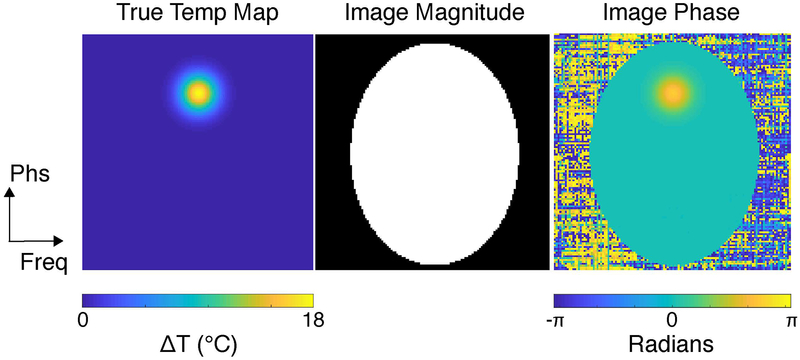
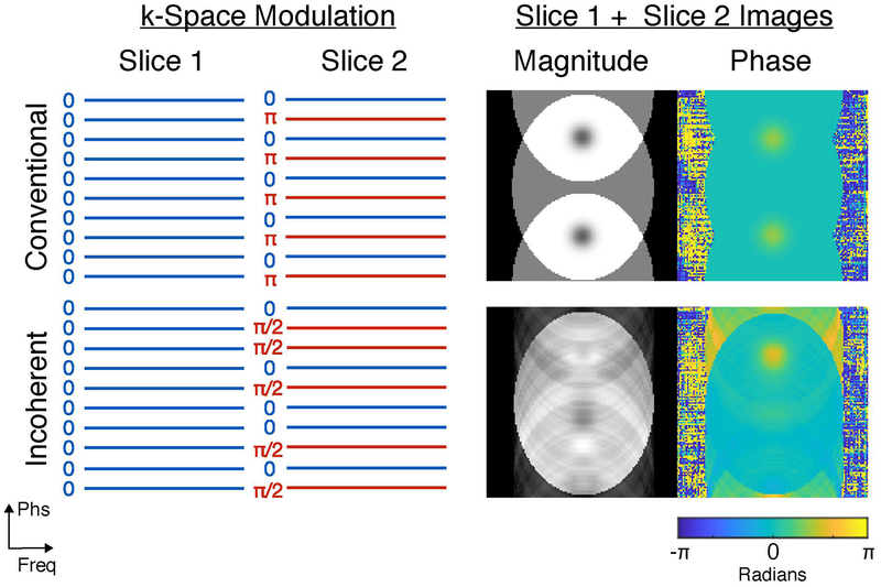
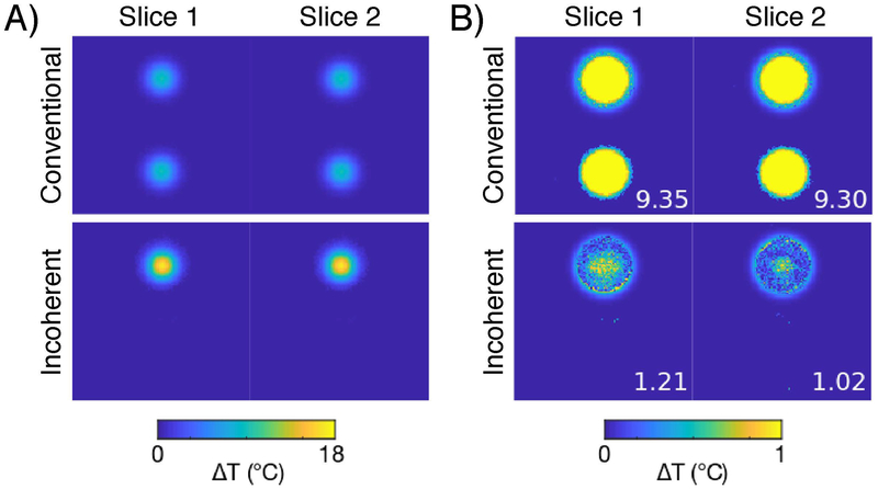
Using the simulation setup shown in Fig. 1 (specific details provided in Methods), Fig. 2 illustrates incoherent-controlled aliasing SMS thermometry via comparison with conventional controlled aliasing-SMS for a multiband (MB) factor of two. In both acquisitions, a multiband pulse is used to excite the two slices, and slice-gradient blips are used to apply phase shifts between them. Without loss of generality, to aid in visualization we assume that the first slice is at isocenter so it experiences no phase shifts. In conventional controlled aliasing-SMS (Fig. 2a, top), the slice-gradient blips apply regular repeating phase shifts across the phase encoding dimension of Slice 2’s k-space signals, to coherently shift Slice 2’s alias in the superimposed image (Fig. 2b, top). This improves the g-factor for parallel imaging-based slice separation [19], compared to applying no inter-slice phase shifts. In incoherent-controlled aliasing SMS, a random pattern of phase shifts (Fig. 2a, bottom) is applied to Slice 2, so the second slice is incoherently aliased in the superimposed image (Fig. 2b, bottom), along with its hot spot which does not appear sparse. This acquisition would typically be unsuitable for parallel imaging-based SMS due to its worse g-factor [21]. However, Figure 3 shows that with a single receive coil, a temperature reconstruction that fits pre-acquired slice-separated baseline images to the incoherent-controlled aliasing data while requiring the temperature maps to be sparse is able to accurately recover slice-separated temperature maps. In contrast, because the aliased conventional controlled-aliasing SMS image contains two coherent, focal hot spots, the same reconstruction is not able to correctly assign the hot spots from that data. In the following sections, we detail the signal model and algorithm underlying this reconstruction.

Figure 1:

Simulation setup. A representative true temperature map is shown on the left. This map was used in all simulations except the slice leakage study. The map contains a Gaussian hot spot with an 8-voxel full-width at half-max, centered FOV/4 from the top of the FOV. The image magnitude used for all slices is shown in the middle, and a representative heating image phase is shown on the right.

Figure 2:

Conventional versus incoherent-controlled aliasing SMS. Conventional controlled aliasing SMS (top) uniformly alternates the phase of Slice 2’s signal across k-space, while incoherent controlled aliasing SMS (bottom) randomly flips Slice 2’s phase. These modulation patterns result in the magnitude and phase images shown on the right. With conventional controlled aliasing SMS, Slice 2 is coherently superimposed on Slice 1 with a FOV/2 shift, resulting in the appearance of two hot spots that are difficult to correctly assign to each slice (Fig. 3). With incoherent controlled aliasing SMS, Slice 2 and its hot spot are smeared incoherently across the FOV, and Fig. 3 shows that the hot spots can be correctly recovered using a sparsity-promoting temperature reconstruction.

Figure 3:

Simulated reconstructed proof-of-concept temperature maps (A) and errors (B). With the same hot spot on both slices, a reconstruction from conventional controlled aliasing SMS data is unable to correctly assign each hot spot, resulting in two partial hot spots in each slice which are visible in the temperature and temperature error maps. In contrast, the reconstruction from incoherent-controlled aliasing SMS data was able to disambiguate the aliasing and correctly assign the hot spots, so that the temperature maps contain full-scale hot spots in their correct locations, and the error maps contain only noise and low-error rings around the hot spots, where the rings result from temperature thresholding applied by the sparsity regularization. In (B), maximum temperature error is reported on each error map. The RMS errors of each reconstruction were 1.80 °C (conventional) and 0.16 °C (incoherent).

Signal Models and Problem Formulations

Here we detail two k-space hybrid multibaseline and referenceless thermometry models for incoherent–controlled aliasing SMS data measured during tcMRgFUS treatment [9, 15]. The general hybrid multibaseline and referenceless model comprises a baseline image measured before heating, which is phase-shifted by a low-order polynomial phase that models respiration and other bulk phase shifts unrelated to heating, and by a focal heating-induced phase. The model implicitly assumes that in the absence of heating, the image magnitudes stay approximately constant. However, in practice this assumption is violated by dynamic and unpredictable changes in water bath signal due to water motion during tcMRgFUS treatment. Specifically, the water moves due to its residual inertia after circulation for cooling is switched off at the start of a sonication, and it can also be perturbed by the FUS beam itself. In previous work, we showed that when k-space data are under-sampled these dynamic changes in water bath signal can alias into the brain and cause temperature errors [12]. In SMS imaging the water bath from one slice will alias into the brain of the other slices, so dynamic changes in water signal will create brain temperature errors in the same way. To avoid this, we simultaneously fit the hybrid model inside the brain and estimate water bath signal changes in each slice. This is done by fitting two models in succession to incoherent-controlled aliasing SMS data. The first model is more general and aggregates both signal changes in the water bath and heating-induced phase shifts in the brain into a single sparsity-regularized complex difference map. The second model is more constrained and enables refinement of the brain heating phase shifts, to eliminate downward temperature bias due to the sparsity regularization in the first model fit. Because of the incoherent slice aliasing in the phase-encoded/k_y dimension, the models are formulated and fit to data in the x−k_y domain.

The first complex difference signal model for the k_y-space data at each x-location is:

$$y^{\delta }\left(k_i^y;w,c,\delta \right)=\sum _{n=1}^{N_{slices}}{e}^{ı{\varphi }_{i,n}}\left[\sum _{j=1}^{N_y}{e}^{ık_i^y{y}_j}\left(\sum _{l=1}^{N_b}{b}_{l,j,n}{w}_l\right)\left(e^{ı{\left\{Ac\right\}}_{j,n}}+{\delta }_{j,n}\right)\right]$$ (1)

where $y^{\delta }\left(k_i^y;w,c,\delta \right)$ is one k-space data sample in the phase-encoded (k_y) dimension, i = 1, .., N_y indexes phase encode lines, n indexes simultaneously imaged slices and N_slices is the multiband factor, $ı=\sqrt{-1}$, and ϕ_i,n is slice n’s controlled-aliasing phase shift at phase encode line i. j indexes the N_y spatial locations in the phase-encoded (y) dimension. The b_l,n are complex-valued slice-separated baseline library images measured prior to treatment, which capture underlying tissue amplitude and phase variations across respiratory and cardiac cycles, and the w_l are baseline image weights, which determine the combination of baseline images that best applies to the current time point. A is a matrix of smooth (low-order polynomial) basis functions and c is a polynomial coefficient vector, which together account for spatially smooth phase changes induced by sources such as center frequency drift and respiration. The δ_n are sparse complex difference maps for each slice that capture complex-valued signal changes due to water bath motion and heating. The x-dependence of y^δ, b, A, and δ is suppressed in Eq. 1 for brevity. To fit this model to a vector of data $\tilde{y}$, the following optimization problem is solved jointly across all x locations:

$$\begin{gathered} \text{minimize }\frac{1}{2}\Vert \tilde{y}-y^{\delta }(w,c,\delta ){\Vert }^2+\lambda {\sum }_{n=1}^{N_{slices}}\Vert {\delta }_n{\Vert }_1 \\ \text{subject to }\sum _{l=1}^{N_b}{w}_l=1 \\ w\succcurlyeq 0, \end{gathered}$$ (2)

where the first term in the objective function is proportional to the negative log-likelihood of the data (when neglecting noise in the baseline images), ‖δ_n‖₁ is the ℓ₁ norm of δ_n, and λ is a regularization parameter that controls the sparsity of the δ_n.

Once the problem in Eq. 2 has been solved to estimate the δ_n, the water bath signal changes in each δ_n are transformed to k-space and subtracted from the data to obtain a modified data vector ${\tilde{y}}^{-\delta }$, and a brain temperature phase shift map θ is initialized to the phase difference between the total complex difference model and the polynomial phase-shifted baseline model term, as:

$${\theta }_{j,n}\leftarrow \angle \left(\sum _{l=1}^{N_b}{b}_{l,j,n}{w}_l\right)\left(e^{ı{\left\{Ac\right\}}_{j,n}}+{\delta }_{j,n}\right){\left(\left(\sum _{l=1}^{N_b}{b}_{l,j,n}{w}_l\right)e^{ı{\left\{Ac\right\}}_{j,n}}\right)}^{*}$$ (3)

for locations j within the brain. Within the brain the baseline images are modified to incorporate the amplitude changes imparted by δ_n, as:

$${\tilde{b}}_{l,j,n}=e^{ı\angle b_{l,j,n}}\left|\left(\sum _{l=1}^{N_b}{b}_{l,j,n}{w}_l\right)\left(e^{ı{\left\{Ac\right\}}_{j,n}}+{\delta }_{j,n}\right)\right|.$$ (4)

Then, a more constrained model is fit with the principal goal of eliminating downward temperature bias due to the sparsity regularization on the δ_n. This model is given by:

$$y^{\theta }\left(k_i^y;w,c,\theta \right)=\sum _{n=1}^{N_{slices}}{e}^{ı{\varphi }_{i,n}}\left[\sum _{j=1}^{N_y}{e}^{ık_i^y{y}_j}\left(\sum _{l=1}^{N_b}{\tilde{b}}_{l,j,n}{w}_l\right)\left(e^{ı{\left\{Ac\right\}}_{j,n}+{\theta }_{j,n}}\right)\right],$$ (5)

which is more constrained than the complex difference model since the complex difference maps δ_n are replaced by phase difference maps θ_n that can capture heating-induced phase shifts but not image magnitude changes. To fit this model to the modified data ${\tilde{\mathit{y}}}^{-\delta }$, the following optimization problem is solved jointly across all x locations:

$$\begin{gathered} \text{minimize }\frac{1}{2}\Vert {\tilde{y}}^{-\delta }-y^{\theta }(w,c,\theta ){\Vert }^2 \\ \text{subject to }{\theta }_n\preccurlyeq 0,n=1,\dots ,N_{slices} \\ \sum _{l=1}^{N_b}{w}_l=1 \\ w\succcurlyeq 0, \end{gathered}$$ (6)

where the non-positivity constraint on the θ_n enforces the prior knowledge that heating will cause negative phase shifts. When solving this problem, the θ_n are only updated in voxels in the brain that had nonzero initial heating phase shifts.

Algorithms

The optimization problems in Eqs. 2 and 6 are both solved using an alternating minimization approach, in which each variable w, c, and δ or θ is updated in turn while holding the others fixed. w is updated by solving a quadratic program, and c and θ are updated using a nonlinear conjugate gradient algorithm, as described in Ref. [9]. The fast iterative soft thresholding algorithm (FISTA) with a constant stepsize is used to update δ (Ref. [22], Eqs. 4.1–4.3).

Methods

Algorithm Implementation

The temperature reconstruction algorithm was implemented in MATLAB R2018 (Mathworks, Natick, MA, USA) on a laptop computer (Apple Macbook Pro, Apple Inc, Cupertino, CA, USA) with a 2.9 GHz Intel Core i7 CPU (Intel Corporation, Santa Clara, CA, USA) and 16 GB of 2133 MHz LPDDR3 RAM. Code and data to implement the algorithm and generate the figures in this work can be downloaded at https://bitbucket.org/wgrissom/k-space-thermometry/. When more than one baseline image was used, the baseline image weights w were solved for using MATLAB’s quadprog function. The polynomial phase coefficient vector c and the complex difference maps δ_n were initialized to zeros. Nonlinear conjugate gradient updates for c used 5 iterations and updates for the phase difference maps θ_n used 10 iterations. The FISTA updates used 50 iterations and a Lipschitz constant/stepsize of 1. One-dimensional fast Fourier transforms were used to transform the spatial domain image models in Eqs. 1 and 5 to k-space. The outer iterations for the complex difference model fit were stopped when the squared-ℓ₂ norm of the change in δ between consecutive iterations fell below 10⁻⁴ times δ’s squared-ℓ₂ norm, and the outer iterations for the phase shift model fit were stopped when the change in the objective function in Eq. 6 fell below 10⁻⁴ times the objective function’s value. To enable similar regularization parameters to be used between reconstructions, the data and baseline images were normalized by the median data amplitude and the square root of the total number of data samples prior to reconstruction. The sparsity regularization parameter λ was also normalized by the number of simultaneous slices.

Simulations

Simulation Setup

Simulations were performed to characterize the maximum number of slices that can be simultaneously imaged, temperature leakage between slices, and robustness across random slice-phase permutations across k-space. Figure 1 shows a representative simulated heating image. The image contains an oval phantom (92 × 120 voxel radii) and a Gaussian-shaped hot spot (full width at half maximum (FWHM) 8 voxels/σ = 10 voxels except in the slice leakage simulation) with a peak phase shift of 3π/4 corresponding to 18 °C heating at 3T with a 16 ms TE, defined on a 128 × 128 matrix. The hot spots were placed FOV/4 (32 voxels) from the center of the image. The same image was used for all slices in all simulations except the slice leakage simulation, to approximate a worst-case imaging scenario in which the slice images are structurally identical. This was based on the expectation that since the proposed SMS method relies on hot spot sparsity, it should be able to reliably separate signals on structurally similar slices. To establish a realistic baseline temperature error, zero-mean additive white complex-valued Gaussian noise was added to the images for a signal-to-noise ratio of 50, based on the measured signal-to-noise ratio of temperature mapping images in the Insightec system used in the below experiments. A single receive coil with uniform sensitivity was used. Temperature reconstructions used one baseline image, a zeroth-order polynomial, and λ = 10⁻².

Incoherent-controlled aliasing SMS k-space data were generated from the simulated heating images by applying randomized phase shift schedules across each slice’s k-space data, and then summing the data across slices. For two and three slices, no phase shifts were applied between the slices for half the phase encodes, and a π/2 phase shift was applied between slices for the other half. For four slices, no phase shifts were applied between the slices for one third of the phase encodes, and π/4 or 3π/4 phase shifts were applied between slices for the other two thirds. For five slices, no phase shifts were applied between slices for one fourth of the phase encodes, and π/4, π/3, or 3π/4 phase shifts were applied between slices for the other three fourths. These phase encoding functions were empirically found to yield improved reconstructed accuracy, compared to randomly permuting the FOV/N_slices phase encoding functions used in conventional controlled-aliasing SMS (results not shown). MATLAB’s randperm function was used to randomly distribute the phase encoding functions across k-space lines. Each simulation was repeated for 50 different permutations, and the same set of permutations was used for all simulations.

Error Versus Number of Slices and Permutations

To characterize the maximum number of slices for which temperature can be simultaneously reconstructed from conventional- and incoherent-controlled aliasing SMS data, simulations of one to five simultaneously imaged slices were performed and root-mean-square (RMS) reconstructed temperature error was calculated for each result. To further characterize robustness across slice-phase permutations, RMS errors were recorded for each permutation for 2 and 3 slices. The conventional controlled-aliasing SMS data were generated by applying phase ramps that shifted successive slices by F OV/N_slices in the phase-encode dimension, prior to summing the slice data.

Slice Leakage

To characterize temperature leakage between slices and its dependence on hot spot size, data were synthesized for two and three slices with a hot spot of varying FWHM on the first slice only. The hot spot FWHM was varied between 8 and 32 voxels, and RMS and peak reconstructed temperature errors were calculated in each slice and across slices.

Experiments

Scanner Implementation

An incoherent-controlled aliasing SMS 2DFT pulse sequence was implemented on a GE Discovery MR750T 3T scanner (GE Healthcare, Waukesha, WI, USA) equipped with an Insightec ExAblate 650 focused ultrasound system (Insightec Ltd, Tirat Carmel, IL), located at the University of Virginia Focused Ultrasound Center. The 2DFT scan used clinically for FUS thermometry (fgre) was modified to incorporate a multiband excitation of two or three slices, and inter-slice π/2 or π phase shifts were applied by reducing the amplitude of the slice rewinder gradient trapezoid, according to a precomputed random schedule across phase encodes. Whenever a phase shift was applied, the slice crusher area was also reduced to maintain constant gradient area each TR. To measure slice-separated baseline images, the first N_slice images were measured using zero, π/2, and π (for three slices) inter-slice phase shifts that were alternated between phase encodes, so that each phase encode was measured with each phase shift. Then slice-separated k-space data were obtained by applying an inverted encoding matrix to each phase encode line’s data. In all scans, the sequence excited 3 mm slices with a 30 degree flip angle, and measured 128 phase encodes and 256 readout samples with a 5.68 kHz readout bandwidth, which are the same settings used clinically. The TE and TR were 13.9 and 27.4 ms, respectively, for a scan time of 3.5 seconds per image. The SMS scans all used 30 mm slice gaps. This value was chosen to avoid signal modulations due to gradient blipping that would result from the larger phase ramps associated with applying slice phases across smaller gaps, and so that any temperature leakage between slices could be easily appreciated in the phantom heating experiments since the hot spots occupied only one slice.

In Vivo Temperature Precision

To characterize temperature precision versus number of slices in vivo, images were acquired in one to three simultaneous axial and sagittal slices during free breathing in a healthy male volunteer outside the water bath, with approval of the Institutional Review Board at the University of Virginia. The subject’s head was supported inside a head birdcage coil, but the scanner’s built-in body coil was used for imaging since it is used for all scans with the transducer. Phase encoding was applied A/P in both orientations. Slice 2 was centered approximately in the hypothalamus in each case, and the scans used a FOV of 240 mm. 50 time points were measured after the baseline data. Temperature reconstructions used four baseline images, a second order polynomial, and λ = 10⁻³. Brain masks were generated for each slice using FSL’s bet tool [23] with manual editing as needed, and in the second model fit temperature phase shifts were estimated in all brain voxels and were not required to be non-positive, to capture both positive and negative temperature errors.

Gel Phantom Heating

To compare single and simultaneous multislice thermometry during heating and in the presence of a water bath, a vendor-provided tissue-mimicking hemispherical quality assurance gel phantom with an 8-cm diameter and an acoustic absorbance of 0.005 Np/mm at 650 kHz was placed in the Insightec system and sonicated while imaging one to three simultaneous axial and sagittal slices. Sonications were started 15 seconds after the scans started, and lasted 30 seconds at 15 Watts acoustic power, with 60% apodization. Slice 2 was centered at the focus, phase encoding was applied A/P in both orientations, and the scans used a FOV of 320 mm. 30 time points were measured after the baseline data. The body coil was used for transmit and receive. Temperature reconstructions used two baseline images, a zeroth order polynomial, and λ = 10⁻². ‘Brain’ masks of the phantom were generated manually in each slice for the second model fit.

Results

Simulations

Error Versus Number of Slices and Permutations

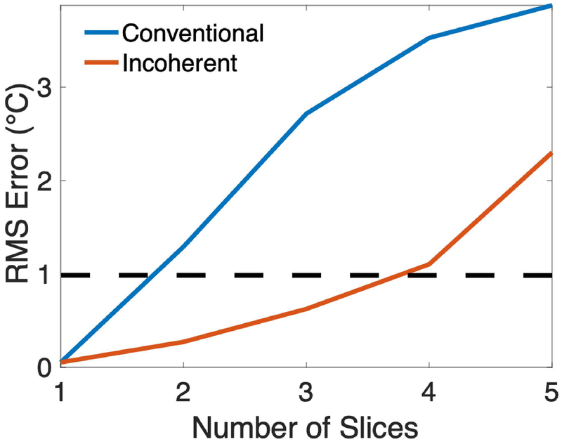
Reconstructed RMS temperature error for conventional-and incoherent-controlled aliasing SMS versus the number of slices is plotted in Figure 4. These errors were calculated inside the phantom across the reconstructed slices and across the 50 k-space phase permutations. Supporting Information Figure S1 plots maximum temperature error versus number of slices, also calculated across reconstructed slices and k-space phase permutations. Using an RMS error of 1 °C as a threshold for acceptable accuracy, incoherent-controlled aliasing enables temperature reconstruction from up to three slices, while no more than one slice can be accurately reconstructed using conventional controlled aliasing SMS. Supporting Information Figure S2 plots RMS and maximum temperature error versus SNR for one slice and for two and three simultaneous slices with incoherent-controlled aliasing, across the 50 k-space phase permutations. The errors vary smoothly with SNR, and RMS errors remain below 1 °C down to an SNR of 10. Supporting Information Figure S3 shows histograms of RMS temperature errors across the 50 different slice-phase permutations. With an acceptable accuracy threshold of 1 °C, 96% and 76% of the permutations produced acceptable accuracy for 2 and 3 slices, respectively.

Figure 4:

Simulated RMS temperature error versus number of slices. For each point, error was calculated across the reconstructed slices within the phantom and across the 50 k-space phase permutations. Setting the acceptable error threshold at an RMS error of 1 °C (dashed line), no more than one slice can be imaged using conventional controlled aliasing SMS, while up to three slices can be imaged simultaneously using incoherent controlled aliasing SMS.

Slice Leakage

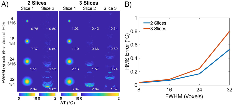
Figure 5a shows temperature maps reconstructed in two and three simultaneously imaged slices, versus hot spot size on the first slice. These maps were selected for being representative across all permutations. Peak temperature errors in each displayed reconstructed slice are reported in white. As the hot spot’s FWHM increased, the peak temperature errors increased both in Slice 1 and in the other slices, but remained at or below 1 °C for a moderately large hot spot with a FWHM of 16 voxels. At a FWHM of 32 voxels (1/4th of the FOV), 42% of the voxels in the phantom are heated more than 1 °C, which is much larger than a typical tcMRgFUS treatment. The peak temperature errors in all slices appear around the perimeter of the hot spot, and there are no coherent hot spot aliases. Figure 5b plots RMS temperature error versus hot spot FWHM, calculated inside the phantom across the reconstructed slices and across the 50 k-space phase permutations; errors remain below 1 °C for all hot spot sizes. Supporting Information Figure S4 plots maximum temperature errors across reconstructed slices and k-space phase permutations. These RMS and maximum error values are lower than those reported in Fig. 4 and Supporting Information Figure S1 because the hot spot is only in Slice 1 in this simulation.

Figure 5:

Simulated hot spot leakage from Slice 1 to Slices 2 and 3, versus hot spot size, for 2- and 3-slice acquisitions. (A) Reconstructed temperature maps for each slice. Note the different color scales for the Slice 1 (0 to 18 °C) versus Slices 2 and 3 (0 to 2 °C). Maximum temperature error is reported in degrees Celsius on each map. (B) RMS temperature error versus hot spot size for 2 and 3 slices. Although errors increased with increasing hot spot size, all RMS errors remained below 1 °C, even for the large FWHM = 32 voxel hot spot that occupied most of the object.

Experiments

In vivo temperature precision

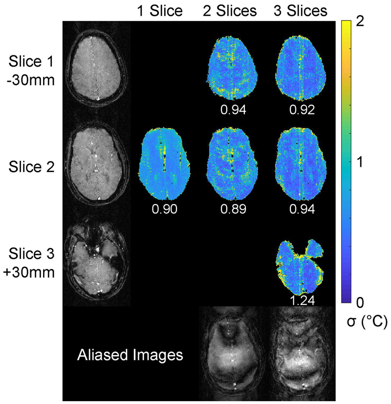
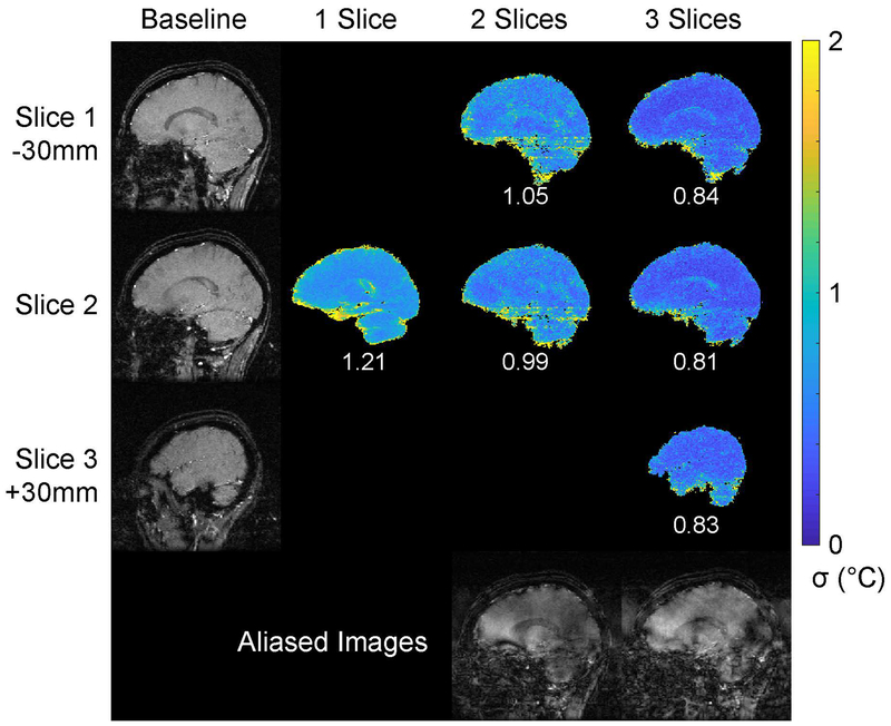
Figure 6 shows axial separated baseline slice images from the 3-slice acquisition and through-time temperature standard deviation maps for each number of simultaneously imaged slices. Representative aliased two- and three-slice images from the time series are also shown, to illustrate the direction of aliasing and the structure of the aliased signals. The baseline images were well-separated with no visible leakage. SMS temperature errors were generally lower than the single-slice acquisition, with the exception of the lowest slice in the three-slice case. Errors were highest near vessels or the edge of the brain, in all cases. Figure 7 shows sagittal separated baseline slice images from the three-slice acquisition, through-time temperature standard deviation maps for each number of simultaneously imaged slices, and representative aliased three-and three-slice images from the time series. The baseline images were again well-separated with no visible leakage. Temperature errors were again lower than the single slice acquisition, though there are some visibly increased errors that streak left-right in the two-slice maps, likely due to pulsating blood vessels. The overall standard deviations of the temperature errors were 1.06 °C (one slice), 0.97 °C (two slices), and 0.93 °C (three slices). The mean temperature errors (i.e., the average value of the deviations from 0 °C) were all below 0.04 °C, reflecting the absence of large static errors across time or space in any of the scans. Supporting Information Videos S1 and S2 show temperature errors through time.

Figure 6:

Axial in vivo temperature standard deviation. Baseline images for each slice are shown in the left column. The slices were separated by 30 mm, with Slice 2 centered on the hypothalamus. The remaining three columns show through-time temperature standard deviation maps for each slice and multiband factor. Overall temperature standard deviation is reported below each slice’s map. Supporting Information Video S1 shows temperature errors at each time point. Slice-aliased images are shown in the bottom row for the two- and three-slice acquisitions.

Figure 7:

Sagittal in vivo temperature standard deviation. Baseline images for each slice are shown in the left column. The slices were separated by 30 mm, with Slice 2 centered on the hypothalamus. The remaining three columns show through-time temperature standard deviation maps for each slice and multiband factor. Overall temperature standard deviation is reported below each slice’s map. Supporting Information Video S2 shows temperature errors at each time point. Slice-aliased images are shown in the bottom row for the two- and three-slice acquisitions.

Gel phantom heating

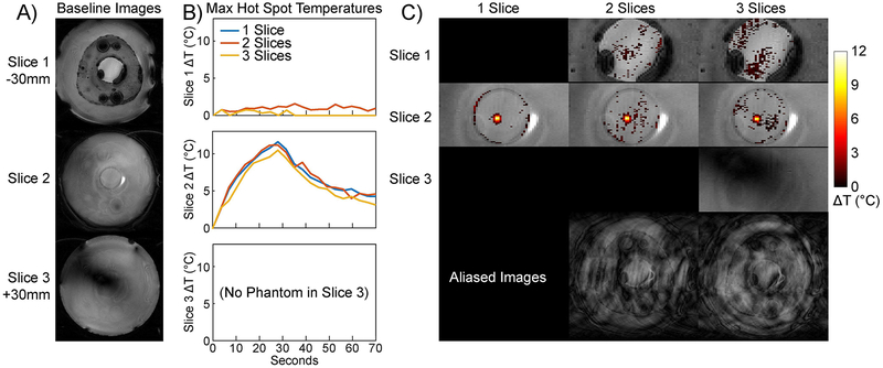
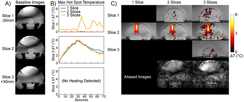
Figure 8a shows axial separated baseline slice images from the three-slice acquisition. The phantom is in the middle of the FOV, and the signal voids above and below the phantom in Slice 1 are caused by air pockets behind the phantom and brass bolts that held the phantom and its plexiglass holder to the Insightec frame. Figure 8b plots maximum temperatures in a 2×2 voxel hot spot mask that was centered on the hot spot in Slice 2 and duplicated to Slices 1 and 3. The SMS maps had low temperatures in Slice 1 where there was no heating, and closely tracked the single-slice hot spot temperature in Slice 2. Figure 8c shows zoomed phantom temperature maps at peak heat in each slice, overlaid on baseline images. The SMS hot spots correspond well to the single slice hot spot and there are no coherent aliases, though there are some small erroneous temperature rises in voxels outside the hot spot that are more frequent in the three-slice map than in the two-slice map. The Figure also shows full-FOV slice-aliased images at this time point for the two- and three-slice acquisitions, to illustrate the aliasing direction and structure. To demonstrate the importance of jointly estimating temperature and water bath signal changes, Supporting Information Figure S5 shows zoomed phantom temperature maps at peak heat in each slice for the two- and three-slice cases, which were reconstructed while ignoring water bath signal changes. In these reconstructions, water bath signal differences from each slice aliased into the phantom in the other slices, where they interfered with the hot spot and produced large temperature errors throughout the phantom. Figure 9a shows sagittal separated baseline slice images from the three-slice acquisition. The phantom is again in the middle of the FOV, and all three slices cut through the phantom. Figure 9b plots maximum temperatures in a 2×11 voxel hot spot mask that was centered on the hot spot in Slice 2 and oriented along its length, and was then duplicated to Slices 1 and 3. The two-slice SMS temperature was near zero in Slice 1, while the the three-slice SMS map had higher errors. In Slice 2, the temperatures closely tracked each other, and no heating was detected in Slice 3 of the three-slice scan. Figure 9c shows zoomed phantom temperature maps at peak heat in each slice, overlaid on baseline images, as well as full-FOV slice-aliased images at this time point for the two- and three-slice acquisitions. The SMS hot spots correspond well to the single slice hot spot and there are no coherent aliases, though there are some small erroneous temperature rises in voxels outside the hot spot that are more frequent in the three-slice map than in the two-slice map. Averaged across all reconstructions, the mean two-slice reconstruction time was 2.1 seconds per time point, and the mean three-slice reconstruction time was 9.1 seconds per time point. Supporting Information Videos S3 and S4 show temperature maps across the sonications.

Figure 8:

Axial phantom heating. (A) Baseline images for each slice. The slices were separated by 30 mm with Slice 2 centered on the focus. Slice 3 contained only water and did not intersect the phantom. (B) Plots of maximum hot spot temperature versus time for each slice, in a 2 × 2 voxel ROI centered on the hot spot in Slice 2 and applied in the same position to all three slices.(C) Temperature maps in each slice at peak heat (30 seconds). Temperature rises above 0.1 °C are overlaid on baseline images that are cropped to the phantom. Supporting Information Video S3 shows temperature maps at each time point. Full-FOV slice-aliased images at this time point are shown in the bottom row for the 2- and 3-slice acquisitions.

Figure 9:

Sagittal phantom heating. (A) Baseline images for each slice. The slices were separated by 30 mm with Slice 2 centered on the focus. (B) Plots of maximum hot spot temperature versus time for each slice, in a 2 × 11 voxel ROI centered on the hot spot in Slice 2 and applied in the same position to all three slices. (C) Temperature maps in each slice at peak heat (30 seconds). Temperature rises above 0.1 °C are overlaid on baseline images that are cropped to the phantom. Supporting Information Video S4 shows temperature maps at each time point. Full-FOV slice-aliased images at this time point are shown in the bottom row for the two- and three-slice acquisitions.

Discussion

We described and evaluated a pulse sequence and temperature map reconstruction algorithm for incoherent-controlled aliasing SMS temperature imaging using a single receive coil. Multiband excitation and blipped-controlled aliasing were implemented in the 2DFT pulse sequence used clinically for tcMRgFUS, and an extended k-space hybrid reconstruction was developed that operates in hybrid x−k_y space and recovers slice-separated temperature maps assuming that heating is sparse, given slice-separated baseline images. The simulations approximated a worst-case scenario in which identical images and hot spots were used for each slice, and showed that under these conditions, two or three slices can be simultaneously imaged while maintaining low temperature errors. Since the baseline images serve a similar role as receive sensitivity maps, the method’s performance is expected to be better when there are more differences between baseline images. In vivo experiments showed little or no loss in temperature precision compared to a single slice scan, for two- and three-slice SMS. Gel phantom heating experiments demonstrated that the two- and three-slice SMS scans yielded hot spot temperatures that closely tracked the single-slice temperature, with no coherent aliasing in other slices.

Our study had a few limitations and opportunities for improvement. One limitation was the lack of an absolute temperature reference such as a fiber optic probe for the phantom heating scans, as this was not compatible with the Insightec gel phantom setup we used. Instead, the conventional clinical 2DFT sequence served as a gold standard. The reconstruction also requires a brain or head mask, to differentiate water bath signal changes from brain signal changes. In practice, brain masks could be obtained by manual outlining, or by magnitude-thresholding or applying bet to images measured before filling the water bath. Currently, our reconstruction is offline, and while the two-slice reconstructions were shorter than the frame rate, the three-slice reconstruction time was too long for online use. The reconstructions could be accelerated by parallelizing operations such as repeated FFT’s across slices. The FISTA algorithm could also be accelerated using backtracking line searches with faster convergence than the fixed step size version used here. We also used the same random permutation of slice-phase encodings across k-space, for every time point in our experiments. However, there may be some benefit to changing permutations between time points. For example, in a retrospective reconstruction, changing permutations would cause leaked signals in the brain to vary at a high frequency through time, so that they could be filtered out using temporal regularization in the reconstruction. If the permutations were structured so that slice-separated images could be reconstructed from two or three consecutive data volumes, then water bath images could be updated in real-time, which may reduce the need for the complex difference component of our reconstruction. This would implicitly assume that the water bath signal changes slowly with respect to the acquisition time. In practice, this assumption would likely be invalid at the beginning of a sonication since the water circulation has just been turned off and the water bath signal changes rapidly, but could work well later in the sonication when the water motion has slowed.

Full volumes of contiguous slices were not imaged in our experiments, but would be of interest to cover a FUS focal zone with slices. In its current form, the proposed SMS scan could immediately be used for near- or far-field monitoring of unintended heating, while simultaneously monitoring the targeted slice. The 30 mm slice gap we used was not optimized but is within the range used in conventional SMS, and was selected to avoid signal modulations due to gradient blipping that would result from the larger phase ramps associated with applying slice phases across smaller gaps, and so that any temperature leakage between slices could be easily appreciated in the phantom heating experiments since the hot spots occupied only one slice. Additionally, with larger slice gaps the method could be useful to accelerate multislice EPI scans for body applications such as prostate ablation [24]; we have previously implemented the blipped-incoherent controlled aliasing method in a multislice EPI sequence on a Philips scanner [17]. Multislice EPI is currently impractical with the GE/Insightec brain system due to limited SNR when using the body coil for imaging, but it could become feasible if new coils become available for the system. It should be possible to make the gaps smaller without significant signal loss due to gradient blipping. Calculations of signal loss depend on the slice profile of the specific RF pulse used for excitation but, for example, assuming an ideal rectangular slice profile and a 3 mm slice thickness, the π/2 inter-slice phase shifts used here could be applied with slice gaps as small as 10 mm, with less than 1% signal loss. It may also be possible to model and account for the effects of low levels of signal loss in the reconstruction, given knowledge of the slice profile and gap. In general, a much smaller slice gap can be used with the proposed method than in conventional SMS, since the temperature reconstruction does not rely on coil sensitivities that become more similar between slices as the gap closes. For zero slice gaps (contiguous slices), the method’s temperature precision should be compared to that of a k-space-undersampled 3D scan.

There are also several possible extensions to this work. First, for applications such as laser brain ablation that still limit the use of dense coil arrays but where there is no water bath, a more constrained phase-only temperature reconstruction could be used (as in the original k-space hybrid method [9]) which can lead to more accurate reconstructions. Second, our reconstruction code can take advantage of more than one coil when available, in which case the reconstruction is equivalent to constrained multiband SENSE [13]. However in that case a careful study should be done to evaluate whether incoherent-controlled aliasing, coherent-controlled aliasing or a combination of the two (for example, coherent in the middle of k-space and incoherent at high frequencies) should be used. At the same time, the proposed method could enable accelerated thermometry on pre-clinical or older MR scanners that don’t have a large number of receive channels. We previously developed an incoherent-controlled aliasing SMS technique that used RF pulses to flip the phases of adjacent slices [16, 18], but this method was found to create unstable signal profiles in time in the water bath due to its long T₁ (data not shown). It could also create unstable signal in cerebrospinal fluid which has a similar T₁. This could be addressed by reordering k-space lines so that flips happen every-other line, as in RF chopping. The RF incoherent-controlled aliasing SMS sequence has the advantage of allowing directly adjacent slices, which could be used to expand volume coverage over the focus and help ensure that the peak heat is captured. When implemented, it should be compared to a 3D scan. For monitoring laser or RF heating where more receive coils may be available, one could also combine this RF-based method with conventional simultaneous multislab imaging given a larger number of receive coils, to achieve higher slice acceleration factors than is possible with either method alone.

Conclusions

Incoherent-controlled aliasing SMS enables accurate reconstruction of focal heating maps from two or three slices simultaneously, using a single receive coil and a sparsity-promoting temperature reconstruction. It can be implemented in the 2DFT MR thermometry imaging sequences used clinically for guiding transcranial MR-guided focused ultrasound, where it maintains the precision and frame rate of a single slice scan but expands volume coverage.

Supplementary Material

Supp VideoS1

Supporting Information Video S1: Axial in vivo temperature errors at each time point. Figure 6 shows the through-time temperature standard deviations of these maps.

Supp VideoS2

Supporting Information Video S2: Sagittal in vivo temperature errors at each time point. Figure 7 shows the through-time temperature standard deviations of these maps.

Supp VideoS3

Supporting Information Video S3: Axial gel phantom temperature at each time point. Figure 8 shows temperature at peak heat.

Supp VideoS4

Supporting Information Video S4: Sagittal gel phantom temperature at each time point. Figure 9 shows temperature at peak heat.

Supp info

Supporting Information Figure S1: Simulated reconstructed maximum temperature error versus number of slices, for conventional- and incoherent-controlled aliasing SMS. For each point, maximum error was calculated across the reconstructed slices and across the 50 k-space phase permutations.

Supporting Information Figure S2: Simulated reconstructed RMS and maximum temperature error versus SNR, for one slice and for two and three simultaneous slices with incoherent-controlled aliasing. For each point, maximum error was calculated across the reconstructed slices and across the 50 k-space phase permutations.

Supporting Information Figure S3: RMS errors of the 50 different random k-space slice-phase permutations used in the two- and three-slice simulations. The red line indicates the 1 °C acceptable error threshold.

Supporting Information Figure S4: Simulated reconstructed maximum temperature error versus hot spot size, for 2 and 3 slices. For each point, maximum error was calculated across the reconstructed slices and across the 50 k-space phase permutations.

Supporting Information Figure S5: Axial phantom temperature maps in each slice at peak heat (30 seconds) for two- and three-slice SMS, when water bath signal changes are ignored in the reconstruction. Temperature rises above 0.1 °C are overlaid on baseline images that are cropped to the phantom.

References

- [1].Elias WJ, Huss D, Voss T, Loomba J, Khaled M, Zadicario E, Frysinger RC, Sperling SA, Wylie S, Monteith SJ, Druzgal J, Shah BB, Harrison M, Wintermark M. A Pilot Study of Focused Ultrasound Thalamotomy for Essential Tremor. New Engl J Med 2013;369:640–648. [DOI] [PubMed] [Google Scholar]
- [2].Ghanouni P, Butts Pauly K, Elias WJ, Henderson J, Sheehan J, Monteith S, Wintermark M. Transcranial MRI-guided focused ultrasound: A review of the technologic and neurologic applications. Am J Roentegnol 2015;205:150–159. [DOI] [PMC free article] [PubMed] [Google Scholar]
- [3].Hughes A, Huang Y, Schwartz ML, and Hynynen K. The reduction in treatment efficiency at high acoustic powers during MR-guided transcranial focused ultrasound thalamotomy for essential tremor. Med Phys 2018;45:2925–2936. [DOI] [PMC free article] [PubMed] [Google Scholar]
- [4].Todd N, Adluru G, Payne A, DiBella EVR, Parker DL. Temporally constrained reconstruction applied to MRI temperature data. Magn Reson Med 2009;62:406–419. [DOI] [PMC free article] [PubMed] [Google Scholar]
- [5].Todd N, Payne A, Parker DL. Model predictive filtering for improved temporal resolution in MRI temperature imaging. Magn Reson Med 2010;63:1269–1279. [DOI] [PMC free article] [PubMed] [Google Scholar]
- [6].Odeen H, de Bever J, Almquist S, Farrer A, Todd N, Payne A, Snell JW, Christensen D, Parker DL Treatment envelope evaluation in transcranial magnetic resonance-guided focused ultrasound utilizing 3D MR thermometry. J Ther Ultrasound 2014;2:19. [DOI] [PMC free article] [PubMed] [Google Scholar]
- [7].Fielden SW, Zhao L, Miller W, Feng X, Wintermark M, Butts Pauly K, Meyer CH. Accelerating 3D spiral MR thermometry with the Kalman filter. In Proc Intl Soc Mag Reson Med. 2014; p. 2346. [Google Scholar]
- [8].Marx M, Plata J, Butts Pauly K. Toward volumetric MR thermometry with the MASTER sequence. IEEE Trans Med Imag 2015;34:148–155. [DOI] [PMC free article] [PubMed] [Google Scholar]
- [9].Gaur P, Grissom WA. Accelerated MRI thermometry by direct estimation of temperature from undersampled k-space data. Magn Reson Med 2015;73:1914–1925. [DOI] [PMC free article] [PubMed] [Google Scholar]
- [10].Jonathan SV, Grissom WA. Volumetric MRI thermometry using a 3D stack-of-stars echo-planar imaging pulse sequence. Magn Reson Med 2018;79:2003–2013. [DOI] [PMC free article] [PubMed] [Google Scholar]
- [11].Gaur P, Partanen A, Werner B, Ghanouni P, Bitton RR, Butts Pauly K, Grissom WA. Correcting heat-induced chemical shift distortions in proton resonance frequency-shift thermometry. Magn Reson Med 2016;76:172–182. [DOI] [PMC free article] [PubMed] [Google Scholar]
- [12].Gaur P, Werner B, Feng X, Fielden SW, Meyer CH, Grissom WA. Spatially-segmented under-sampled MRI temperature reconstruction for MR-guided focused ultrasound. J Therapeutic Ultrasound 2017;5:13. [DOI] [PMC free article] [PubMed] [Google Scholar]
- [13].Barth M, Breuer F, Koopmans PJ, Norris DG, Poser BA. Simultaneous multislice (SMS) imaging techniques. Magn Reson Med 2016;75:63–81. [DOI] [PMC free article] [PubMed] [Google Scholar]
- [14].Borman PTS, Bos C, de Boorder T, Raaymakers BW, Moonen CTW, Crijns SPM. Towards real-time thermometry using simultaneous multislice MRI. Phys Med Biol 2016;61:N461–N477. [DOI] [PubMed] [Google Scholar]
- [15].Grissom WA, Rieke V, Holbrook AB, Medan Y, Lustig M, Santos J, McConnell MV, Pauly KB. Hybrid referenceless and multibaseline subtraction MR thermometry for monitoring thermal therapies in moving organs. Med Phys 2010;37:5014–5026. [DOI] [PMC free article] [PubMed] [Google Scholar]
- [16].Poorman ME, Quah K, Grissom WA. Simultaneous multislice MRI thermometry with incoherent caipirinha and sparsity-promoting reconstruction. In Proceedings ISTU 2018;. [Google Scholar]
- [17].Quah K, Poorman ME, Grissom WA. Simultaneous multislice MRI temperature imaging with a single receive coil. In Proceedings BMES 2018; p. 2790. [Google Scholar]
- [18].Quah K, Poorman ME, Grissom WA. Simultaneous multislice MRI temperature imaging with a single receive coil. In Proceedings 27th Scientific Meeting, International Society for Magnetic Resonance in Medicine, Montreal 2019; p. 801. [Google Scholar]
- [19].Setsompop K, Gagoski BA, Polimeni JR, Witzel T, Wedeen VJ, Wald LL. Blipped-controlled aliasing in parallel imaging for simultaneous multislice echo planar imaging with reduced g-factor penalty. Magn Reson Med 2012;67:1210–24. [DOI] [PMC free article] [PubMed] [Google Scholar]
- [20].Zur Y, Wood ML, Neuringer LJ. Spoiling of transverse magnetization in steady-state sequences. Magn Reson Med 1991;21:251–263. [DOI] [PubMed] [Google Scholar]
- [21].Zhu K, Dougherty RF, Wu H, Middione MJ, Takahashi AM, Zhang T, Pauly JM, Kerr AB. Hybrid–space SENSE reconstruction for simultaneous multi-slice MRI. IEEE Trans Med Imag 2016;35:1824–1836. [DOI] [PMC free article] [PubMed] [Google Scholar]
- [22].Beck A, Teboulle M. A fast iterative shrinkage-thresholding algorithm for linear inverse problems. Siam J Imaging Sciences 2009;2:183–202. [Google Scholar]
- [23].Smith SM. Fast robust automated brain extraction. Human Brain Mapping 2002;17:143–155. [DOI] [PMC free article] [PubMed] [Google Scholar]
- [24].Burtnyk M, Hill T, Cadieux-Pitre H, Welch I. Magnetic resonance image guided transurethral ultrasound prostate ablation: A preclinical safety and feasibility study with 28-day followup. J Urol 2015;193:1669–1675. [DOI] [PubMed] [Google Scholar]
Associated Data
This section collects any data citations, data availability statements, or supplementary materials included in this article.
Supplementary Materials