

Abstract
Classifying different object categories is one of the most important aims of brain–computer interface researches. Recently, interactions between brain regions were studied using different methods, such as functional and effective connectivity techniques. Functional and effective connectivity techniques are applied to estimate human brain areas connectivity. The main purpose of this study is to compare classification accuracy of the most advanced functional and effective methods in order to classify 12 basic object categories using Electroencephalography (EEG) signals. In this paper, 19 channels EEG signals were collected from 10 healthy subjects; when they were visiting color images and instructed to select the target images among others. Correlation, magnitude square coherence, wavelet coherence (WC), phase synchronization and mutual information were applied to estimate functional cortical connectivity. On the other hand, directed transfer function, partial directed coherence, generalized partial directed coherence (GPDC) were used to obtain effective cortical connectivity. After feature extraction, the scalar feature selection methods including T-test and one-sided-anova were applied to rank and select the most informative features. The selected features were classified by a one-against-one support vector machine classifier. The results indicated that the use of different techniques led to different classifying accuracy and brain lobes analysis. WC and GPDC are the most accurate methods with performances of 80.15% and 64.43%, respectively.
Keywords: Object recognition, Electroencephalography (EEG), Functional connectivity, Effective connectivity, Brain connectivity
Introduction
Classifying different object categories is one of the most significant aspects of brain–computer interface (BCI); for recognition and classifying object categories we need informative features that can discriminate classes. There are several types of features that have the ability to classify categories, but recently there have been a growing interest to extract discriminative features from human brain areas connectivity.
There are three types of brain connectivity: structural connectivity characterizes the brain regions anatomical connectivity, functional connectivity is described as the relations and interactions between separated brain areas; effective connectivity refers to directed influence of one neural system on others (Fingelkurts et al. 2005; Horwitz 2003). Functional and effective connectivity provides us the knowledge for better understanding the brain function, while functional connectivity evaluates the temporal correlation of different active brain regions, effective connectivity evaluates how activity of one region influence the other separated regions.
EEG as a non-invasive recording technique is being widely applied to real-time decoding of the human brain function (Müller et al. 2008). EEG is able to distinguish different brain states, specifically processing of distinct semantic categories (Proverbio et al. 2007). In analyzing EEG signals, feature extraction (Ince et al. 2005), feature selection (Lal et al. 2004) and classification techniques (Peters et al. 2001) are the most important aspects that can be considered. Different types of classifiers are used for classifying the data, such as multilayer perceptron (MLP) (Richiardi et al. 2010) and decision trees (Richiardi et al. 2011), but this research used SVM (Ethofer et al. 2009) for classifying data. Recently, as an important part of the classification, brain connectivity feature extraction techniques have been developed. These techniques are used to develop modeling of the brain at the same time to be used for clinical applications. A number of previous researches studied the changes in brain areas connectivity of unhealthy people. Scientists provided algorithms for distinguishing healthy and unhealthy people by comparing their brain connectivity. For example, Li et al. (2015) studied patients with depression during emotional face processing, they found that patients’ functional connectivity of EEG gamma band is different from normal people. Their abnormal functional connectivity was estimated by calculating EEG coherence. In another study, Lee et al. (2014) evaluated brain functional connectivity of post-traumatic stress disorder (PTSD) patients by Mutual Information (MI). The results of the study indicated that resting-state functional connectivity of these people is decreased dependent to PTSD symptom severity. Also, Nasrolahzadeh et al. used information from nonlinear spontaneous speech signals to introduce a frame to classify 30 Alzheimer patients and 30 healthy control participants. They used higher order spectral features for analysis, four classifiers for classification subjects into three different levels of Alzheimer’s disease and healthy groups and Ten-fold cross-validation procedure to estimate the validity of the classifier outcomes. They understood that the introduced frame can properly diagnose Alzheimer’s disease, especially the earliest stage of the disease (Nasrolahzadeh et al. 2018). Moreover, Hejazi and Nasrabadi evaluated brain effective connectivity and found that near Epilepsy seizure these connections have major changes which can be used as a sign to predict the seizure. They applied directed transfer function (DTF) and Granger Causality (GC) techniques to measure two time-variant coefficients and compared them over the time. The results indicates that the obtained value of accuracy and sensitivity are higher than values in other studies (Hejazi and Nasrabadi 2019). Also, Wu et al. (2012) analyzed the effect of Guqin music on brain functional connectivity by applying graph theory. Their analysis showed music perception increased functional connectivity.
In Several studies, functional and effective connectivity were used for evaluating brain functions and activities during a special task. For example, Parhizi et al. evaluated functional and effective connectivity of the brain in a spatial-based task by applying Coherence and GC techniques and obtaining graph theory measures such as degree and characteristic path length. They found as the outcomes that somatosensory, parietal, prefrontal areas and visual cortex have connections to other parts of the cortex during the task. Also, Characteristic path length demonstrated that increase of functional connectivity and functional integration in spatial-based attention is more than feature-based attention (Parhizi et al. 2018). In another study, Mora-Sánchez et al. assessed different hypothesises about the brain regions engagement approaches in joint activity by using EEG. They offered a frame that explains brain-state switches are discrete, but according to volume conduction the EEG recordings show these switches are influenced by neighboring areas (Mora-Sánchez et al. 2019). Moreover, Déli et al. illustrated that there are some frequency couplings between slow and fast oscillations of the neurons in the brain. According to their topological findings the microscopic neural activities can predict single activities in much larger levels (Déli et al. 2017). Also, Liu et al. used EEG to demonstrate differences among activities of brain areas in people with high creativity in comparison with those who have low creativity during presentation of a text stimuli. They found out that by different word stimuli brain activation can discriminate participants into these two groups (Liu et al. 2018). Also, Myers and Kozma adopted a mesoscopic brain activity model, in which regions of the limbic system are represented by networks. The model illustrates seizure behaviour of limbic system regions while increasing external weights that join all networks (Myers and Kozma 2018).
In several papers, emotional states were classified by EEG based brain connectivity, for example Khosrowabadi et al. (2010) conducted a research on recognition of four emotional states from EEG signals by MI and magnitude square coherence (MSC) during audio-visual emotional stimuli. Also, Lee and Hsieh (2014) classified three emotional states by estimating EEG based functional connectivity. They used Correlation, Phase Synchronization (PS) and Coherence to estimate functional connectivity. The study indicated in different emotional states functional connectivity changed significantly. Moreover, Chen et al. (2015) used Correlation, MI and phase coherence to estimate EEG connectivity among electrodes to identify participants’ affective levels in arousal and valence dimensions. They found that MI provided the best information for classifying arousal and valence. The results indicated that Gamma band connectivity features are more informative for valence level classification.
A number of papers published their studies about object recognition, for instance Wang et al. (2016) evaluated functional connectivity patterns in object recognition of four categories including Faces, Scenes, Animals and Tools based on fMRI and they found discriminative network for each category. Moreover, Martinovic et al. (2008) evaluated object features role in an object recognition study. They demonstrated that features of objects coded very fast in different neural systems and the mentioned features have different functional roles in the object recognition process, while the edges and colors delay it. In another object categorization study using event related potential, Tanaka and Curran (2001) found that objects from domain of expertise of adults are neurologically different from objects outside their domain of expertise. Also, Amedi et al. (2005) reviewed cross modal object recognition researches that used fMRI; These researches indicated visual, auditory and tactile information of objects can activate cortical areas that were believed to be modality-specific. The study proposed that the recruitment and location of multisensory convergence zones are depended on the information content and the dominant modality.
A number of studies applied EEG signals for recognition. For example, Khasnobish et al. used EEG signals of 15 blindfolded participants for 3-D texts recognition during tactile exploration. Different classifiers in hierarchical one-versus-one approach were applied to classify extracted features up to six classes. The results indicates when the number of classes increases the classification accuracy decreases, which is because of the mental overload (Khasnobish et al. 2017). In other study, Taghizadeh-Sarabi et al. (2015) used EEG signals for object recognition and feature extraction techniques such as wavelets, but rather they did not use feature extraction methods based on brain connectivity. Just one work has been done, applying brain connectivity for object recognition with fMRI (Wang et al. 2016). We used EEG because it can straightforwardly evaluate oscillation patterns in frequency bands which is the cause of functional and effective connectivity in brain. Also, EEG is more affordable and available in compared to fMRI. Several researches applied EEG signals and brain connectivity feature extraction for classification, yet these studies did not classify objects. For example, they classified different emotions (Khosrowabadi et al. 2010). To the best of authors’ knowledge, our study is the first study that used EEG based functional and effective connectivity for object recognition and compared the classification accuracy of these approaches.
The main aim of this study is twofold. First, we extracted features from recorded EEG signals by applying the most advanced functional and effective connectivity feature extraction techniques to classify images of 12 basic categories. Second, we compared classification accuracy of functional and effective connectivity techniques in order to find which features are more informative for discrimination of the classes.
The remainder of this paper is organized as follows. Second section methods and materials are described. Third section discusses the experimental results. Finally, the conclusion is represented in fourth section.
Methodology
Participants and ethics statement
Ten healthy subjects with normal vision (2 female, 8 male; mean age: 23 ± 3.4 years) participated in the experiment after informing the task and signing the written consent form, according to the Helsinki principles. All were right-handed except one. The experiment was approved by the National Committee of Ethics in Medical Research (Taghizadeh-Sarabi et al. 2015).
Stimuli and experiment
Color images of 12 categories including animals, flowers, fruit, transportation devices, body organs, clothing, food, stationery, buildings, electronic devices, dolls and jewelry were displayed to participants. All images were 600 × 800 pixels. Figure 1 indicates all 12 categories of images.
Fig. 1.
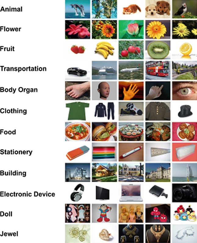
All 12 categories. All Categories including animal, flower, fruit, transportation device, body organ, clothing, food, stationery, building, electronic device, doll and jewel are represented
The experiment was run in two parts with a three-min break between the parts. In the first part, six categories were displayed, and the second part remained categories were displayed with a fixed order for all participants. Totally 360 images were exhibited during an experiment to each subject. Each category included 30 images; with 15 related images and 15 unrelated ones that were chosen from other categories; Non-target images were randomly displayed among the related ones. The images were displayed only once for each participant without any information about their orders. Figure 2 illustrates the order of displaying images. In the experiment before each category a word, which is named target cue, was displayed. In order to prevent from interference of motor signals with others, subjects were asked to press the left mouse button with their right hand if the shown image belonged to target category right after 700 ms of stimulus presentation and during the 800 ms time interval otherwise do nothing.
Fig. 2.

The order of images in the experiment. Target cue is presented on the screen for 1 s, then after 900 ms. showing a black screen, each image is displayed for 700 ms with an 800 ms delay between consecutive images
Target cue was shown on the screen for 1 s, then after 900 ms showing a black screen the image was displayed for 700 ms. There was an 800 ms delay between consecutive images; subjects were asked to delay their blinks in this interval. Between categories a black screen was presented for 5 s. All the images were displayed on an LCD monitor. Procedure of displaying images was managed by a PC running PSYTASK-WinEEG presentation software. PSYTASK is a software for presenting visual/audio stimuli; it is used with WinEEG, which makes the stimuli presentation and EEG signals recording synchronized.
EEG data collection
EEG signals were collected with 19-channel electrode cap, according to the International 10-20 system of electrode placement, with linked-ears montage (Miller et al. 1991). Figure 3 indicates the order of se lected channels (FP1, FP2, F3, F4, C3, C4, P3, P4, F7, F8, T3, T4, T5, T6, FZ, CZ, PZ, O1, and O2). EEG signals were amplified with MITSAR hardware then they were sent through an analog-to-digital converter. The signals were recorded with sampling rate of 500 Hz.
Fig. 3.

The order of EEG Recording channels. EEG signals were recorded from 19 channel electrodes
Preprocessing
After collecting EEG signals, in order to accomplish better performance, they should be preprocessed. EEG signals were filtered by a 1–50 Hz phase-shift free Butterworth band-pass filter. Moreover, slow waves with voltages higher than 50 µv and fast waves with voltages higher than 30 µv were removed by MATLAB software (Saeid and Chambers 2007). The eye movement removing was done by independent component analysis (ICA) of WinEEG.
The first 40 ms of the EEG signals from the image onset was, and the 660 ms remained signals were used for processing. The 40 ms was removed, because information reaches to the primary visual cortex after about 40–50 ms. The 660 ms signal converted to 330 samples according to 500 Hz frequency sampling rate. Due to 19 EEG channels, one single trial dimension equals 19 × 330. By analyzing the first 660 ms of the signals that were simultaneous with image presentation, it is possible that a combined response from the brain areas related to visual stimuli and working memory (because of showing the target category name before the stimuli) arises. So it is not possible to make a distinction between these two types of activities. It is possible to select the signals from 800 ms interval between the images and label them same as their previous stimuli; if the results of categorizing these signals be similar to those from 660 ms stimulus presentation, it can be concluded that working memory effect is the prominent response. In case of lack of the similarities it can be said that results are belonged to visual stimuli.
As mentioned, EEG signals were collected from 10 subjects. According to unmanageable artifacts in the 4th and 5th participants’ signals, collected data from these subjects were not used for further analysis.
Feature extraction
After preprocessing the signals, EEG based functional and effective brain connectivity was estimated by the most advanced methods and used as features for classifying categories.
In order to extract features, firstly the connectivity matrices were calculated for each of the observations; each observation was a matrix of 19 × 330 (for 19 channels and 660 ms of signal with sampling rate of 500 Hz). The intended connectivity feature was assessed on each pair of channels, for example, calculating the correlation between channels resulted in a 19 × 19 channels matrix that array (i, j) illustrated the correlation value between channel i, j. Secondly, to convert each connectivity matrix to a row in the feature matrix for functional (undirected) method the top 19 × 18/2 array of the connectivity matrix were put sequentially in a row, and whole 19 × 19 array were used as features of the effective (directed) methods.
Functional connectivity
Functional connectivity is a description of observed correlations; it does not describe how these correlations are mediated. It was estimated using the correlation of EEG signals for the first time in 1960 (Friston and Buchel 2003; Brazier and Casby 1952; Adey et al. 1961). In this study, functional connectivity of brain areas was extracted using different techniques including Wavelet Coherence (WC), Correlation, MSC, PS and MI.
Wavelet coherence (WC)
WC is a qualitative estimator that provides the temporal evolution of relations between signals with a given scale (Labat 2005). The wavelet transform of a signal is a function of frequency and time, which is produced by the convolution of the signal with a defined Wavelet family :
| 1 |
The Wavelet cross-spectrum between signals and around time and frequency is defined by the Wavelet transforms of and :
| 2 |
* defines the complex conjugate and is assumed as a scalar which depends on frequency. WC at the time and frequency is described by
| 3 |
where is cross spectral density between and ; is the auto-correlation of signal and is the auto-correlation of signal at time and frequency (Van Milligen et al. 1995).
Correlation
Pearson correlation coefficient of two signals is obtained by dividing the cross-covariance of the two variables by the product of their auto-covariance and (Miller et al. 1991; Saeid and Chambers 2007). The Pearson correlation coefficient ranges from − 1 to 1. A higher correlation means a stronger relationship between brain regions.
| 4 |
Magnitude square coherence (MSC)
The MSC is a linear synchronization approach which gives a value ranges between 0 and 1 to detect how well x corresponds to y at frequency f (Berkman et al. 2004). A higher estimated MSC indicates stronger linear interdependency between brain areas. The MSC is defined as follows:
| 5 |
where is cross power spectral density, and are the power spectral density of the two different signals and (Carter et al. 1973; Sakkalis 2011).
Phase synchronization (PS)
PS assumes two oscillation systems without amplitude synchronization can have phase synchronization. The instantaneous phase of signal is given by:
| 6 |
where is the Hilbert transform of which is defined as:
| 7 |
where PV refers to the Cauchy principal value. The Phase locking value for two signals is defined as:
| 8 |
where defines the sampling period and indicates the sample number of each signal (Stam et al. 2007; Mormann et al. 2000). PS index value ranges from 0 to 1, Where 0 shows lack of synchronization and 1 indicates strict phase synchronization.
Mutual information (MI)
According to Information Theory, MI of two random variables shows how a random variable is informative for the other one. Let, and be the probability distributions of random variables and , respectively. The entropy of and are defined as:
| 9 |
| 10 |
where n defines window length. and are conditional entropy and joint entropy between and , respectively. They are defined as:
| 11 |
| 12 |
where is the expected value function. MI of two random variables and is computed as follows (Khosrowabadi et al. 2010):
| 13 |
if and only if random variables and are statistically independent.
Effective connectivity
Effective connectivity can be defined as the influence of a neural system on other neural systems for performing motor, cognitive and perceptual functions. These functions show complex interactions, which can be bidirectional or unidirectional coupling in brain regions. In synchronized neural systems, both systems have the same rhythm, whereas there can be causal interaction between neural systems (Zervakis et al. 2011; Delorme et al. 2002). This kind of connectivity can be synaptic or cortical (Friston 1994). In this study, DTF, Partial Directed Coherence (PDC) and Generalized Partial Directed Coherence (GPDC) were used to estimate effective connectivity of the brain regions.
Directed transfer function (DTF)
DTF was introduced as a method to estimate information flow in 1991. This method is based on the concept of GC estimated on multivariate autoregressive model (MVAR), which models all signals simultaneously (Kaminski and Blinowska 1991). According to the concept of GC, time series is cause of time series if the past information of decrease the prediction error of at the present time (Kamiński et al. 2001). It indicates the direction of information flow because predictability is not reciprocal. is a set of estimated signals from recording channels:
| 14 |
The MVAR process is an expressive description of the data set :
| 15 |
In this model is a zero mean multivariate uncorrelated white noise vector with . is coefficients matrix and represent the border of the model. Equation (15) is transformed into frequency domain which is defined as:
| 16 |
where
| 17 |
Equation (16) can be changed to:
| 18 |
is the transfer function of the system and its elements indicate the causal influence from the jth input to the ith output at frequency f. The DTF is defined as:
| 19 |
Normalized DTF is defined as:
| 20 |
where describes influence ratio of the jth channel related cortical area on the ith channel related cortical area respect to the influence of all estimated cortical signals (Babiloni et al. 2005). Normalized DTF value ranges from 0 to 1 when
| 21 |
Partial directed coherence (PDC)
PDC is a method which quantifies the relation between 2 among signals, avoiding volume conduction by estimating influences of all other signals. PDC improves the concept of Partial Coherence by estimating directional (i.e. causal) influences. This method is estimated on MVAR.
is a set of estimated signals from recording channels:
| 22 |
The MVAR process is an expressive description of the data set :
| 23 |
In this model is a zero mean multivariate uncorrelated white noise vector. is the autoregressive coefficients matrix and its elements indicates the influence of on and represents the border of the model. PDC from the ith channel to the jth channel at frequency f is defined as follows:
| 24 |
where is frequency domain description of (Granger 1969).
| 25 |
where describes the influence ratio of the jth channel on the ith channel respect to the influence of all estimated cortical signals (Babiloni et al. 2005). PDC value ranges from 0 to 1.
Generalized partial directed coherence (GPDC)
GPDC is defined as follows by normalizing Eq. (24) by standard deviation (Schelter et al. 2006; Baccala et al. 2006).
| 26 |
Feature selection
All features were normalized after Feature extraction. There are several methods that could be used to reduce the number of features and select the best features for classifying images such as Genetic Algorithm, mRMR, infinite feature selection, t-test, one-sided-anova and etc. (Adams et al. 2017); in this study, two methods were used; The first one was based on t-test criterion and the second one was one-sided-anova. In t-test method, features are ranked according to t-test criterion. The value shows how a feature is suitable for separating two classes. This method is enabled to classify images in two classes. According to 12 classes in this study, the method was used for all possible states 66 (C (12 2)) times. Finally, the most repeated features were ranked. The best number of features was indicated by comparing classification accuracy for different number of features.
On the other hand, one-sided-anova that uses F distribution to compare means of many samples was applied. The returned p value was used to select the best features. In this study, features with p value < 0.01 were selected.
It should be mentioned that in order prevent from seeing the effects of test data in training data-set, feature selection has been done on training data within each repetition of cross validation scheme that will be discussed more in the significance test section.
It should be mentioned that instead of using t-test or anova, it is also usual to determine the significant connections between the EEG channels even before starting any other process, by applying the Surrogate control analysis on data (this can be evaluated in the further studies), but in this study first, we calculated the connectivity between each pairs of the channels by assuming them as significant connection and then we selected the principal connections by applying t-test and one-sided-anova on the full-weighted graph.
Classification
A Support Vector Machine (SVM) is a classifier that uses separating hyperplane for discriminating classes (Guler and Ubeyli 2007). In this study, we used “one-against-one” strategy which makes an SVM classifier for each two classes. “one-against-one” strategy, which is applied in the cases with less training data can make better classifying accuracy than “one-against-all” strategy (Milgram et al. 2006). Moreover, different influences of SVM kernels were evaluated on obtaining classification accuracy; and Radial Basis Function (RBF) was chosen as the kernel function due to its higher performance. This nonlinear kernel can map samples to a higher dimension to make a situation to classify samples (Hsu et al. 2003). Equation (11) shows the mentioned kernel as follows:
| 27 |
where indicates the width of the kernel.
Significance test
In k-fold cross-validation, the data is randomly separated into k equal sized sub-data without overlapping. One of these sub-data is used as the test data and the remaining k − 1 sub-data is used as training data. This procedure will be repeated k times, each time with a new test data. Finally the result is the average of all k accuracies.
In this study, fivefold cross-validation was used to randomly separate the data into five equal sized sub-data without overlapping. One sub-data was used as the test (validation) data and the remaining four sub-data are used as training data. In other words, all data was decomposed into 80% training data and 20% test data. Each time feature selection process, using the methods which were described earlier, had been done on fourfolds of training data and the selected features were chosen in onefold of test data to evaluate the classifier’s accuracy This procedure was repeated five times and the result was the average of all five accuracies. It should be mentioned that because of the small number of data, it was not possible to separate the data into 3 groups in order to provide an external (hold-out) test dataset, so the whole procedure was an internal cross-validation.
SVM parameters
One of the most important parts of this study was optimizing the SVM parameters, regularization constant and kernel arguments. The C parameter is used for trading off misclassification against the complexity of the discriminant hyperplane. A high C classifies the training data correctly by a complex discriminant surface while a low C performances vice versa. Finding optimal value for SVM parameters was done for each participant separately.
Results and discussion
The experimental design and the applied methods were explained in “Methodology” section. As it was mentioned, the main aim of this study is evaluation and comparing different methods of feature extraction based on functional and effective connectivity in classifying 12 object categories from EEG signals of eight participants. Object categories are as follows: animals, flowers, fruit, transportation devices, body organs, clothing, food, stationery, buildings, electronic devices, dolls and jewelry, respectively from category number 1 to number 12.
Finding optimal SVM parameters was done separately for each subject and each feature extraction technique. In Fig. 4 SVM parameters optimization for subject 1 using WC is shown. Searching for the best values for regularization constant and kernel argument is done by a grid-search over SVM parameters to find the best test data classification accuracy. The figure indicates that (6.30, 6.30) is the best choice for regularization constant and kernel argument, respectively.
Fig. 4.
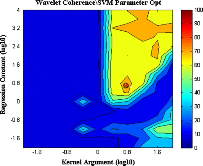
Optimization of SVM parameters. Searching for the best values for regularization constant and kernel argument is done by finding the best classification accuracy for WC method. The best choice for regularization constant and kernel argument is (6.30, 6.30)
After finding the best values for SVM parameters, the optimal number of features for t-test criterion is necessary. The optimal number of features is indicated by comparing obtained accuracies for different number of features. Figure 5 illustrates accuracy comparison for finding the optimal number of features for WC.
Fig. 5.
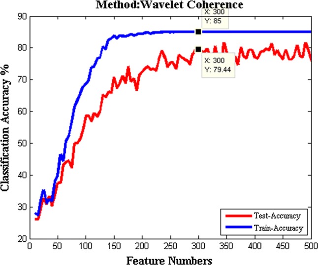
The optimal number of features based on t-test criterion. The optimal number of features is shown as 300 because of the best test and train data classification accuracies on (300, 79.44) and (300, 85), respectively
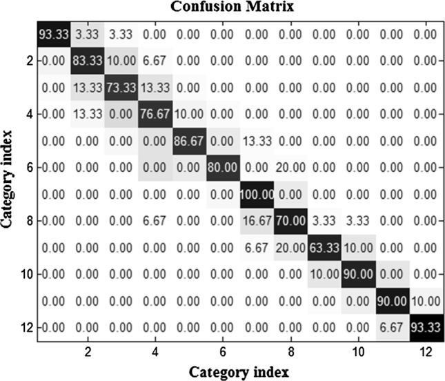
For better understanding the discrimination of categories, we used confusion matrix (CM). Each column of the CM illustrates the predicted class and each row indicates the actual class. Firstly, In order to calculate the CM the test data were given to the trained SVM classifier and the predicted outputs from the classifier were compared with actual labels. Then, for each category the numbers of correct and incorrect predictions were calculated and the cells in each row were filled in. Finally, to convert the numbers to percentage rates, the numbers in each row were divided by sum of all numbers in that row and multiplied by 100. For example, for category 1 the percentage of correct predictions was written in cell (row = 1, column = 1) of CM, and the percentage of the data that were belonged to category 1 but were classified as category 2 was put in cell (1, 2), and so forth for other cells in the first row. It is clear that for the cells from the second to twelfth rows, the predicted labels of test data from second to twelfth categories were evaluated similar to the first row. Figure 6 indicates the CM, which is an average matrix for confusion matrices of all subjects using WC and one-sided-anova. It is clear that the best classification accuracy is related to category of animals and the worst one is relevant to transportation devices with accuracy percentages of 100 and 33.33, respectively.
Fig. 6.
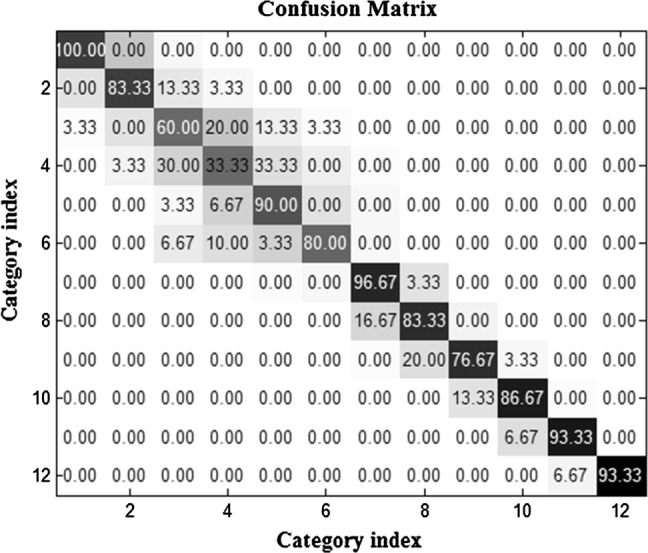
The averaged confusion matrix using WC and one-sided-anova. The best classification accuracy is related to category of animals with accuracy percentage of 100
Figure 7 indicates classification accuracies; each accuracy is an average for confusion matrices of all subjects using WC and t-test criterion. The best classification is allocated to recognition category of 100 and 63.33, respectively. In order to understand the influence of feature selection techniques, Figs. 6 and 7 can be compared. It is clearly seen that different feature selection methods led to different classification accuracies in 12 categories, by selecting different discriminative features.
Fig. 7.
The averaged confusion matrix using WC and t-test. The best classification accuracy is allocated to category of food
Figure 8 depicted the averaged brain lobes connectivity matrices using WC and t-test. It is clearly shown that the most connectivity was observed in temporal-frontal and central-frontal lobes. The results are rational by considering function of the brain lobes; Object recognition, which was evaluated in this study is one of the temporal lobe functions. Moreover, decision making is related to the frontal lobe and in the experiment participants made decision to the task to categorize the images.
Fig. 8.
The averaged brain lobes connectivity matrix for all subjects using WC and t-test. The most connectivity was observed in temporal–frontal and central–frontal lobes
The averaged classification accuracies of all subjects are reported in Table 1 for all functional and effective connectivity feature extraction techniques and two scalar features selection methods, separately. All the accuracies have higher values than chance level (Combrisson and Jerbi 2015). (In a 12-class classification problem, the chance level is calculated as:.)
Table 1.
The averaged classification accuracies (%) of all subjects using functional and effective connectivity feature extraction
| Feature extraction techniques | Feature selection methods | |
|---|---|---|
| T-test | One-sided-anova | |
| WC | 80.15 | 71.34 |
| Correlation | 50.15 | 45.37 |
| MSC | 47.62 | 44.70 |
| PS | 57.92 | 51.41 |
| MI | 53.48 | 44.00 |
| DTF | 62.17 | 56.85 |
| PDC | 60.21 | 53.52 |
| GPDC | 64.43 | 58.38 |
The best classification accuracy allocated to WC feature extraction method and t-test criterion
It is obviously seen that the best accuracy allocates to WC as functional feature extraction method and GPDC as an effective feature extraction method with accuracy percentages of 80.15 and 64.43, respectively. Frequency domain feature extraction techniques had better results. According to higher classification accuracies, features based on effective connectivity were more informative. Comparing feature selection methods indicate that t-test criterion was able to choose more informative features and led to higher accuracies.
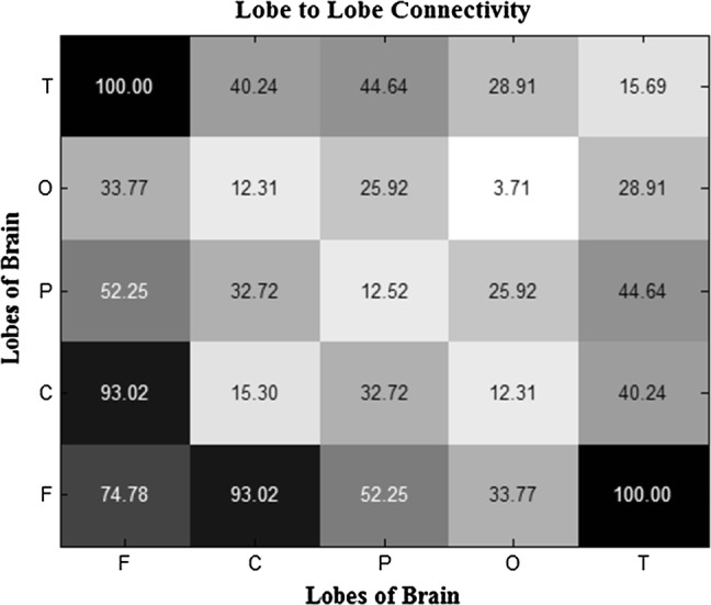
Figure 9 indicates the average of brain lobes connectivity matrices, which were formed using all functional feature extraction techniques and feature selection based on t-test criterion, for all subjects. It should be mentioned that T, O, P, C and F are symbols for Temporal, Occipital, Parietal, Central and Frontal lobes of the brain, respectively. Connectivity had more strength between frontal-frontal, frontal-central and frontal-temporal lobes, while connectivity between parietal-occipital and parietal-parietal lobes was the weakest.
Fig. 9.

The averaged brain lobes connectivity matrix using all functional feature extraction techniques and feature selection based on t-test criterion. Connectivity had more strength between frontal–frontal, frontal–central and frontal–temporal lobes
In Fig. 10 indicates the average of brain lobes connectivity matrices, which is the result of using all effective feature extraction techniques and feature selection based on t-test criterion, for all subjects. Connectivity had more strength between parietal-parietal, occipital-occipital and temporal-temporal lobes, while connectivity between parietal-occipital was the weakest.
Fig. 10.
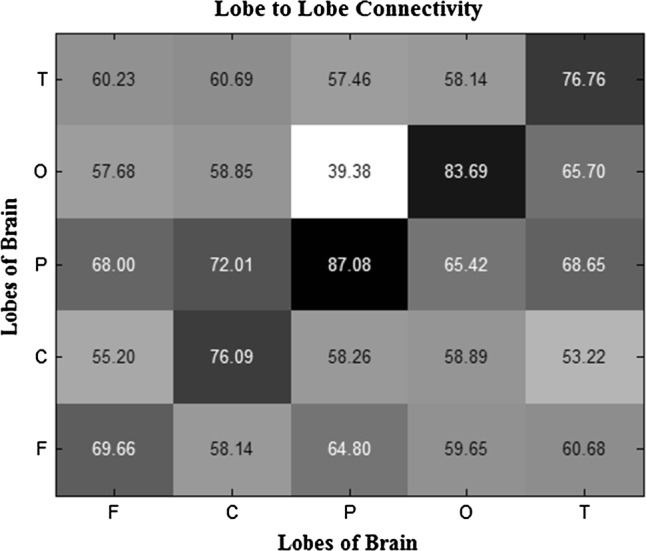
The averaged brain lobes connectivity matrix using all effective feature extraction techniques and feature selection based on t-test criterion. Connectivity had more strength between parietal–parietal, occipital–occipital and temporal–temporal lobes
Conclusion
The main aim of this study is to indicate how well functional and effective brain connectivity is informative as features for classification. For this purpose, human brain areas connectivity was applied for classifying 12 basic object categories by using 19 channels EEG signals. ICA and filtering were done on the signals recorded from 8 participants, as preprocessing. Features were extracted applying five functional connectivity techniques including Correlation, MSC, WC, PS and MI and three effective connectivity techniques, such as DTF, PDC and GPDC. In order to select the best features of connectivity two scalar feature selection methods including t-test and one-sided-anova were used. Finally, a multiclass SVM with “one-against-one” strategy and optimized parameters was used to classify the selected features. To the best of authors’ knowledge, our study is the first study that used EEG based functional and effective connectivity for object recognition and compared the classification accuracy of these approaches. WC and GPDC were recognized as the most accurate methods with accuracy percentages of 80.15 and 64.43, respectively. It is clearly seen that the functional and effective techniques which were in frequency domain achieved better classification accuracy than those in time domain. Brain lobes connectivity was illustrated for all feature extraction techniques and feature selection methods separately.
Footnotes
Publisher's Note
Springer Nature remains neutral with regard to jurisdictional claims in published maps and institutional affiliations.
References
- Adams S, Meekins R, Beling PA (2017) An empirical evaluation of techniques for feature selection with cost. In: 2017 IEEE international conference on data mining workshops (ICDMW). IEEE, pp 834–841
- Adey WR, Walter DO, Hendrix CE. Computer techniques in correlation and spectral analyses of cerebral slow waves during discriminative behavior. Exp Neurol. 1961;3(6):501–524. doi: 10.1016/S0014-4886(61)80002-2. [DOI] [PubMed] [Google Scholar]
- Amedi A, von Kriegstein K, van Atteveldt NM, Beauchamp MS, Naumer MJ. Functional imaging of human crossmodal identification and object recognition. Exp Brain Res. 2005;166(3–4):559–571. doi: 10.1007/s00221-005-2396-5. [DOI] [PubMed] [Google Scholar]
- Babiloni F, Cincotti F, Babiloni C, Carducci F, Mattia D, Astolfi L, Basilisco A, Rossini PM, Ding L, Ni Y, Cheng J. Estimation of the cortical functional connectivity with the multimodal integration of high-resolution EEG and fMRI data by directed transfer function. Neuroimage. 2005;24(1):118–131. doi: 10.1016/j.neuroimage.2004.09.036. [DOI] [PubMed] [Google Scholar]
- Baccala LA, Takahashi DY, Sameshima K (2006) Computer intensive testing for the influence between time series. In: Schelter B, Winterhalder M, Timmer J (eds) Handbook of time series analysis-recent theoretical developments and applications. pp 411–436
- Berkman E, Wong DK, Guimaraes MP, Uy ET, Gross JJ, Suppes P (2004) Brain wave recognition of emotions in EEG. In: Psychophysiology, vol 41. Blackwell Publishing Ltd, Oxford, pp S71–S71
- Brazier MA, Casby JU. Crosscorrelation and autocorrelation studies of electroencephalographic potentials. Electroencephalogr Clin Neurophysiol. 1952;4(2):201–211. doi: 10.1016/0013-4694(52)90010-2. [DOI] [PubMed] [Google Scholar]
- Carter G, Knapp C, Nuttall A. Estimation of the magnitude-squared coherence function via overlapped fast Fourier transform processing. IEEE Trans Audio Electroacoust. 1973;21(4):337–344. doi: 10.1109/TAU.1973.1162496. [DOI] [Google Scholar]
- Chen M, Han J, Guo L, Wang J, Patras I (2015) Identifying valence and arousal levels via connectivity between EEG channels. In: 2015 International conference on affective computing and intelligent interaction (ACII). IEEE, pp 63–69
- Combrisson E, Jerbi K. Exceeding chance level by chance: the caveat of theoretical chance levels in brain signal classification and statistical assessment of decoding accuracy. J Neurosci Methods. 2015;250:126–136. doi: 10.1016/j.jneumeth.2015.01.010. [DOI] [PubMed] [Google Scholar]
- Déli E, Tozzi A, Peters JF. Relationships between short and fast brain timescales. Cogn Neurodyn. 2017;11(6):539–552. doi: 10.1007/s11571-017-9450-4. [DOI] [PMC free article] [PubMed] [Google Scholar]
- Delorme A, Makeig S, Fabre-Thorpe M, Sejnowski T. From single-trial EEG to brain area dynamics. Neurocomputing. 2002;44:1057–1064. doi: 10.1016/S0925-2312(02)00415-0. [DOI] [Google Scholar]
- Ethofer T, Van De Ville D, Scherer K, Vuilleumier P. Decoding of emotional information in voice-sensitive cortices. Curr Biol. 2009;19(12):1028–1033. doi: 10.1016/j.cub.2009.04.054. [DOI] [PubMed] [Google Scholar]
- Fingelkurts AA, Fingelkurts AA, Kähkönen S. Functional connectivity in the brain—is it an elusive concept? Neurosci Biobehav Rev. 2005;28(8):827–836. doi: 10.1016/j.neubiorev.2004.10.009. [DOI] [PubMed] [Google Scholar]
- Friston KJ. Functional and effective connectivity in neuroimaging: a synthesis. Hum Brain Mapp. 1994;2(1–2):56–78. doi: 10.1002/hbm.460020107. [DOI] [Google Scholar]
- Friston KJ, Buchel C. Functional connectivity. Hum Brain Funct. 2003;2:999–1018. [Google Scholar]
- Granger CW. Investigating causal relations by econometric models and cross-spectral methods. Econometrica. 1969;37(3):424–438. doi: 10.2307/1912791. [DOI] [Google Scholar]
- Guler I, Ubeyli ED. Multiclass support vector machines for EEG-signals classification. IEEE Trans Inf Technol Biomed. 2007;11(2):117–126. doi: 10.1109/TITB.2006.879600. [DOI] [PubMed] [Google Scholar]
- Hejazi M, Nasrabadi AM. Prediction of epilepsy seizure from multi-channel electroencephalogram by effective connectivity analysis using Granger causality and directed transfer function methods. Cogn Neurodyn. 2019;13(5):461–473. doi: 10.1007/s11571-019-09534-z. [DOI] [PMC free article] [PubMed] [Google Scholar]
- Horwitz B. The elusive concept of brain connectivity. Neuroimage. 2003;19(2):466–470. doi: 10.1016/S1053-8119(03)00112-5. [DOI] [PubMed] [Google Scholar]
- Hsu CW, Chang CC, Lin CJ (2003) A practical guide to support vector classification. Paper available at http://www.csie.ntu.edu.tw/~cjlin/papers/guide/guide.pdf
- Ince NF, Tewfik A, Arica S (2005) Classification of movement EEG with local discriminant bases. In: Proceedings of IEEE international conference on acoustics, speech, and signal processing, 2005 (ICASSP’05), vol 5. IEEE, pp v-413
- Kaminski MJ, Blinowska KJ. A new method of the description of the information flow in the brain structures. Biol Cybern. 1991;65(3):203–210. doi: 10.1007/BF00198091. [DOI] [PubMed] [Google Scholar]
- Kamiński M, Ding M, Truccolo WA, Bressler SL. Evaluating causal relations in neural systems: granger causality, directed transfer function and statistical assessment of significance. Biol Cybern. 2001;85(2):145–157. doi: 10.1007/s004220000235. [DOI] [PubMed] [Google Scholar]
- Khasnobish A, Datta S, Bose R, Tibarewala DN, Konar A. Analyzing text recognition from tactually evoked EEG. Cogn Neurodyn. 2017;11(6):501–513. doi: 10.1007/s11571-017-9452-2. [DOI] [PMC free article] [PubMed] [Google Scholar]
- Khosrowabadi R, Heijnen M, Wahab A, Quek HC (2010) The dynamic emotion recognition system based on functional connectivity of brain regions. In: 2010 IEEE intelligent vehicles symposium (IV). IEEE, pp 377–381
- Labat D. Recent advances in wavelet analyses: part 1. A review of concepts. J Hydrol. 2005;314(1):275–288. doi: 10.1016/j.jhydrol.2005.04.003. [DOI] [Google Scholar]
- Lal TN, Schroder M, Hinterberger T, Weston J, Bogdan M, Birbaumer N, Scholkopf B. Support vector channel selection in BCI. IEEE Trans Biomed Eng. 2004;51(6):1003–1010. doi: 10.1109/TBME.2004.827827. [DOI] [PubMed] [Google Scholar]
- Lee YY, Hsieh S. Classifying different emotional states by means of EEG-based functional connectivity patterns. PLoS ONE. 2014;9(4):e95415. doi: 10.1371/journal.pone.0095415. [DOI] [PMC free article] [PubMed] [Google Scholar]
- Lee SH, Yoon S, Kim JI, Jin SH, Chung CK. Functional connectivity of resting state EEG and symptom severity in patients with post-traumatic stress disorder. Prog Neuropsychopharmacol Biol Psychiatry. 2014;51:51–57. doi: 10.1016/j.pnpbp.2014.01.008. [DOI] [PubMed] [Google Scholar]
- Li Y, Cao D, Wei L, Tang Y, Wang J. Abnormal functional connectivity of EEG gamma band in patients with depression during emotional face processing. Clin Neurophysiol. 2015;126(11):2078–2089. doi: 10.1016/j.clinph.2014.12.026. [DOI] [PubMed] [Google Scholar]
- Liu YC, Chang CC, Yang YHS, Liang C. Spontaneous analogising caused by text stimuli in design thinking: differences between higher-and lower-creativity groups. Cogn Neurodyn. 2018;12(1):55–71. doi: 10.1007/s11571-017-9454-0. [DOI] [PMC free article] [PubMed] [Google Scholar]
- Martinovic J, Gruber T, Müller MM. Coding of visual object features and feature conjunctions in the human brain. PLoS ONE. 2008;3(11):e3781. doi: 10.1371/journal.pone.0003781. [DOI] [PMC free article] [PubMed] [Google Scholar]
- Milgram J, Cheriet M, Sabourin R (2006) “One against one” or “one against all”: which one is better for handwriting recognition with SVMs? In: Tenth international workshop on frontiers in handwriting recognition. Suvisoft
- Miller GA, Lutzenberger W, Elbert T. The linked-reference issue in EEG and ERP recording. J Psychophysiol. 1991;5(3):273–276. [Google Scholar]
- Mora-Sánchez A, Dreyfus G, Vialatte FB. Scale-free behaviour and metastable brain-state switching driven by human cognition, an empirical approach. Cogn Neurodyn. 2019;13(5):437–452. doi: 10.1007/s11571-019-09533-0. [DOI] [PMC free article] [PubMed] [Google Scholar]
- Mormann F, Lehnertz K, David P, Elger CE. Mean phase coherence as a measure for phase synchronization and its application to the EEG of epilepsy patients. Physica D. 2000;144(3):358–369. doi: 10.1016/S0167-2789(00)00087-7. [DOI] [Google Scholar]
- Müller KR, Tangermann M, Dornhege G, Krauledat M, Curio G, Blankertz B. Machine learning for real-time single-trial EEG-analysis: from brain–computer interfacing to mental state monitoring. J Neurosci Methods. 2008;167(1):82–90. doi: 10.1016/j.jneumeth.2007.09.022. [DOI] [PubMed] [Google Scholar]
- Myers MH, Kozma R. Mesoscopic neuron population modeling of normal/epileptic brain dynamics. Cogn Neurodyn. 2018;12(2):211–223. doi: 10.1007/s11571-017-9468-7. [DOI] [PMC free article] [PubMed] [Google Scholar]
- Nasrolahzadeh M, Mohammadpoory Z, Haddadnia J. Higher-order spectral analysis of spontaneous speech signals in Alzheimer’s disease. Cogn Neurodyn. 2018;12(6):583–596. doi: 10.1007/s11571-018-9499-8. [DOI] [PMC free article] [PubMed] [Google Scholar]
- Parhizi B, Daliri MR, Behroozi M. Decoding the different states of visual attention using functional and effective connectivity features in fMRI data. Cogn Neurodyn. 2018;12(2):157–170. doi: 10.1007/s11571-017-9461-1. [DOI] [PMC free article] [PubMed] [Google Scholar]
- Peters BO, Pfurtscheller G, Flyvbjerg H. Automatic differentiation of multichannel EEG signals. IEEE Trans Biomed Eng. 2001;48(1):111–116. doi: 10.1109/10.900270. [DOI] [PubMed] [Google Scholar]
- Proverbio AM, Del Zotto M, Zani A. The emergence of semantic categorization in early visual processing: ERP indices of animal vs. artifact recognition. BMC Neurosci. 2007;8(1):24. doi: 10.1186/1471-2202-8-24. [DOI] [PMC free article] [PubMed] [Google Scholar]
- Richiardi J, Van De Ville D, Eryilmaz H (2010) Low-dimensional embedding of functional connectivity graphs for brain state decoding. In: 2010 First workshop on brain decoding: pattern recognition challenges in neuroimaging (WBD). IEEE, pp 21–24
- Richiardi J, Eryilmaz H, Schwartz S, Vuilleumier P, Van De Ville D. Decoding brain states from fMRI connectivity graphs. Neuroimage. 2011;56(2):616–626. doi: 10.1016/j.neuroimage.2010.05.081. [DOI] [PubMed] [Google Scholar]
- Saeid S, Chambers JA. EEG signal processing. Chichester: Willey; 2007. [Google Scholar]
- Sakkalis V. Review of advanced techniques for the estimation of brain connectivity measured with EEG/MEG. Comput Biol Med. 2011;41(12):1110–1117. doi: 10.1016/j.compbiomed.2011.06.020. [DOI] [PubMed] [Google Scholar]
- Schelter B, Winterhalder M, Eichler M, Peifer M, Hellwig B, Guschlbauer B, Lücking CH, Dahlhaus R, Timmer J. Testing for directed influences among neural signals using partial directed coherence. J Neurosci Methods. 2006;152(1):210–219. doi: 10.1016/j.jneumeth.2005.09.001. [DOI] [PubMed] [Google Scholar]
- Stam CJ, Nolte G, Daffertshofer A. Phase lag index: assessment of functional connectivity from multi channel EEG and MEG with diminished bias from common sources. Hum Brain Mapp. 2007;28(11):1178–1193. doi: 10.1002/hbm.20346. [DOI] [PMC free article] [PubMed] [Google Scholar]
- Taghizadeh-Sarabi M, Daliri MR, Niksirat KS. Decoding objects of basic categories from electroencephalographic signals using wavelet transform and support vector machines. Brain Topogr. 2015;28(1):33–46. doi: 10.1007/s10548-014-0371-9. [DOI] [PubMed] [Google Scholar]
- Tanaka JW, Curran T. A neural basis for expert object recognition. Psychol Sci. 2001;12(1):43–47. doi: 10.1111/1467-9280.00308. [DOI] [PubMed] [Google Scholar]
- Van Milligen BP, Sanchez E, Estrada T, Hidalgo C, Brañas B, Carreras B, Garcia L. Wavelet bicoherence: a new turbulence analysis tool. Phys Plasmas (1994-present) 1995;2(8):3017–3032. doi: 10.1063/1.871199. [DOI] [Google Scholar]
- Wang X, Fang Y, Cui Z, Xu Y, He Y, Guo Q, Bi Y. Representing object categories by connections: evidence from a mutivariate connectivity pattern classification approach. Hum Brain Mapp. 2016;37(10):3685–3697. doi: 10.1002/hbm.23268. [DOI] [PMC free article] [PubMed] [Google Scholar]
- Wu J, Zhang J, Liu C, Liu D, Ding X, Zhou C. Graph theoretical analysis of EEG functional connectivity during music perception. Brain Res. 2012;1483:71–81. doi: 10.1016/j.brainres.2012.09.014. [DOI] [PubMed] [Google Scholar]
- Zervakis M, Michalopoulos K, Iordanidou V, Sakkalis V. Intertrial coherence and causal interaction among independent EEG components. J Neurosci Methods. 2011;197(2):302–314. doi: 10.1016/j.jneumeth.2011.02.001. [DOI] [PubMed] [Google Scholar]