MULTILAYER KNOCKOFF FILTER: CONTROLLED VARIABLE SELECTION AT MULTIPLE RESOLUTIONS

Abstract

We tackle the problem of selecting from among a large number of variables those that are “important” for an outcome. We consider situations where groups of variables are also of interest. For example, each variable might be a genetic polymorphism, and we might want to study how a trait depends on variability in genes, segments of DNA that typically contain multiple such polymorphisms. In this context, to discover that a variable is relevant for the outcome implies discovering that the larger entity it represents is also important. To guarantee meaningful results with high chance of replicability, we suggest controlling the rate of false discoveries for findings at the level of individual variables and at the level of groups. Building on the knockoff construction of Barber and Candès [Ann. Statist. 43 (2015) 2055–2085] and the multilayer testing framework of Barber and Ramdas [J. Roy. Statist. Soc. Ser. B 79 (2017) 1247–1268], we introduce the multilayer knockoff filter (MKF). We prove that MKF simultaneously controls the FDR at each resolution and use simulations to show that it incurs little power loss compared to methods that provide guarantees only for the discoveries of individual variables. We apply MKF to analyze a genetic dataset and find that it successfully reduces the number of false gene discoveries without a significant reduction in power.

1. Introduction.

1.1. A motivating example.

During the last 20 years the biotechnology that allows us to identify the locations where the genome of an individual is different from a reference sequence has experienced a dramatic increase in speed and decrease in costs. Scientists have used the resulting wealth of information to investigate empirically how variations in our DNA translate into different measurable phenotypes. While we still know little about the causal mechanisms behind many traits, geneticists agree on the usefulness of a multivariate (generalized) linear model to capture at least as a first approximation the nature of the relation between genetic variation and complex phenotypes. If $\mathbf{y}\in {ℝ}^{n\times 1}$ is the vector collecting the values of a quantitative trait in n subjects, and $\mathit{X}\in {ℝ}^{n\times N}$ the matrix storing, column by column, their genotypes at N polymorphic sites in the genome, a starting model for their relation is

$$\mathit{y}=\mathit{X}\mathit{\beta }+\mathit{\epsilon },$$

where the coefficients $\mathit{\beta }\in {ℝ}^{N\times 1}$ represent the contributions of measured genetic variations to the trait of interest. We remark on a few characteristics of this motivating genetic application: (1) The adjective “complex” referring to a trait is to be interpreted as non-Mendelian, that is, influenced by many different genetic variants, we expect several of the elements of β to be nonzero, and we can exploit this fact using multiple regression models. (2) The main goal of these studies is the identification of which β_j ≠ 0. In other words the focus is not on developing a predictive model for y, but on selecting important variables that represent the biological mechanism behind the trait and whose relevance can be observed across multiple datasets. (3) Recognizing that β_j ≠ 0 corresponds to scientific discoveries at multiple levels, each column of X represents a single genetic variant, but these are organized spatially in meaningful ways and their coefficients also give us information about coarser units of variation. For example, a number of adjacent polymorphisms might all map to the same gene, the portion of DNA coding for a protein. If the coefficient for any of these polymorphisms is different from zero, then we can conclude that the gene is important for the trait under study. This type of discovery is relevant to advancing our understanding of the biology behind a trait. At the same time, knowing which specific variant influences the phenotype is also relevant; this is the type of information we need for precise clinical testing and genetic counseling.

In summary, an ideal solution would identify important genetic variants accounting for their interdependence, and provide error control guarantees for the discovery of both variants and genes. The work in this paper attempts to achieve this goal. We emphasize that similar problems occur in contexts other than genetics. Modern methods of data acquisition often provide information on an exhaustive collection of possible explanatory variables, even if we know a priori that a large proportion of these are not relevant for our outcome of interest. In such cases we rely on statistical analysis to identify the important variables in a manner that facilitates replicability of results while achieving appreciable power. Replication of findings in separate independent studies is the cornerstone of science and cannot be substituted by a type of statistical analysis. Furthermore, the extent to which results replicate depends not only on how the conclusions were drawn from the original data but also on the characteristics of the follow-up study: Does it have enough power? Does it target exactly the same “population” of the original investigation? etc…. Yet, controlling Type-I error is a necessary step toward replicability, important in order to avoid wasting time and money on confirmatory follow-up studies of spurious findings. Finally, it is often the case that we measure variables at a very fine resolution and need to aggregate these measurements for meaningful interpretation. We consider three examples in addition to our primary motivating application.

fMRI studies.

Consider, for example, studies that investigate the role of different brain structures. With functional magnetic resonance imaging (fMRI) we measure on the order of a million voxels at regular time intervals during an experiment. These measurements might then be used in a model of neurocognitive ability. Usually, measurements from nearby voxels are aggregated and mapped to recognizable larger-scale brain structures called regions of interest [Poldrack (2007)]. With a time dimension also involved, we can group (voxel, time) pairs spatially or temporally. It then becomes important to make sure that the statistical methods we adopt guarantee reproducibility with respect to each kind of scientifically interpretable finding.

Multifactor analysis-of-variance problems with survey data.

In social science multiple choice surveys are frequently employed in order to gather information about some characteristics of subjects. The results of these surveys can be viewed as predictor variables for certain outcomes, such as income. Since the different answer choices for a given question are coded as separate dummy variables, it makes sense to study the importance of an entire question by considering all the variables corresponding to the same question. However, if a particular question is discovered to be significantly associated with an outcome, then it might also be of interest to know which answer choices are significant. Hence, an analysis at the level of questions (groups of variables) and answer choices (individual variables) is appropriate [Yuan and Lin (2006)].

Microbiome analysis.

The microbiome (the community of bacteria that populate specific areas of the human body, such as the gut or mouth) has gained attention recently as an important contributing factor for a variety of human health outcomes. By sequencing the bacterial 16S rRNA gene from a specimen collected from a human habitat, it is possible to quantify the abundances of hundreds of bacterial species. Bacteria, like other living organisms, are organized into hierarchical taxonomies with multiple layers including phylum, class, family and so on. It is of interest to find associations between health outcomes and the abundances of different types of bacteria, as described with each layer of the taxonomic hierarchy [Sankaran and Holmes (2014)].

1.2. Statistical challenges.

Having motivated our problem with several applications, we give an overview of the statistical challenges involved and of the tools we will leverage.

Controlled variable selection in high dimensional regression.

In a typical genome wide association study (GWAS) the number of subjects n is on the order of tens of thousands, and the number N of genetic variants (in this case single nucleotide polymorphisms, or SNPs) is on the order of a million. To provide finite sample guarantees of global error, geneticists typically analyze the relation between X and y using a series of univariate regressions of y on each of the columns of X, obtain the p-values for the corresponding t-tests and threshold them to achieve family wise error rate (FWER) control. This analysis is at odds with the polygenic nature of the traits, and the choice of FWER as a measure of global error makes it difficult to recover a substantial portion of the genetic contribution to the phenotype [Manolio et al. (2009)]. Using a multiple regression model for analysis and targeting false discovery rate (FDR) [Benjamini and Hochberg (1995)] are promising alternatives.

Unfortunately, in a context where N > n these are difficult to implement. Regularized regression, including the lasso [Tibshirani (1996)] and various generalizations, for example, Simon et al. (2013), Yuan and Lin (2006), have proven to be very versatile tools with nice prediction properties, but they do not come with model selection guarantees in finite samples [for examples of asymptotic properties see Knight and Fu (2000), Negahban et al. (2009)]. Recent years have seen progress on this front. While in general it is difficult to obtain p-values for high-dimensional regression, Javanmard and Montanari (2014) propose a construction that is valid under certain sparsity assumptions. Alternatively, conditional inference after selection [Fithian, Sun and Taylor (2014), Taylor and Tibshirani (2015)] can also be used in this context. The idea is to first reduce dimensionality by a screening method and then to apply the Benjamini Hochberg (BH) procedure to p-values that have been adjusted for selection [Markovic, Xia and Taylor (2017)]. Other approaches have been proposed that bypass the construction of p-values entirely. SLOPE is a modification of the lasso procedure which provably controls the FDR under orthogonal design matrices [Bogdan et al. (2015)] and has been applied to GWAS, allowing for a larger set of discoveries which, at least in the analyzed examples, have shown good replicability properties [Brzyski et al. (2017)]. The knockoff filter [Barber and Candès (2015), Candès et al. (2018)]—which is based on the construction of artificial variables to act as controls—guarantees FDR control for variable selection in a wide range of settings. We will review the properties of knockoffs in Section 2.2, as we will leverage them in our construction.

Controlling the false discovery rate at multiple resolutions.

While the standard GWAS analysis results in the identification of SNPs associated with a trait, geneticists also routinely rely on gene level tests based on the signal coming from multiple variants associated to the same coding region [Santorico and Hendricks (2016) is a recent review], as well as other forms of aggregate tests based on pathways [see Wang, Li and Bucan (2007), e.g.]. Unfortunately, each of these approaches represents a distinct analysis of the data, and the results they provide are not necessarily consistent with each other. We might find association with a SNP, but not with the gene to which it belongs, or with a gene, but with none of the variants typed in it. Moreover, multiple layers of analysis increase the burden of multiple testing, often without this being properly accounted for. Yet, geneticists are very interested in controlling type I errors, as follow-up studies are very time consuming and diagnosis and counseling often need to rely on association results before a thorough experimental validation is possible.

In this context, we want to investigate all the interesting levels of resolution simultaneously [e.g., Zhou et al. (2010)] and in a consistent fashion, providing meaningful error control guarantees for all the findings. The fact that we have chosen FDR as a measure of error rate makes this a nontrivial endeavor. Unlike FWER, FDR is a relative measure of global error, and its control depends crucially on how one defines discoveries. As we discuss in Section 2.1, a procedure that guarantees FDR control for the discovery of single variants does not guarantee FDR control for the discoveries of genes. This has been noted before in contexts where there is a well defined spatial relationship between the hypotheses, and the discoveries of scientific interest are at coarser resolution than the hypotheses tested (e.g., MRI studies [Benjamini and Heller (2007), Poldrack (2007)], genome scan statistics [Siegmund, Zhang and Yakir (2011)] and eQTL mapping [GTEx Consortium et al. (2015)]). Proposed solutions to these difficulties vary depending on the scientific context, the definition of relevant discoveries and the way the space of hypotheses is explored; Benjamini and Bogomolov (2014), Bogomolov et al. (2017), Heller et al. (2018), Yekutieli (2008) explore hypotheses hierarchically, while Barber and Ramdas (2017) and Ramdas et al. (2017) consider all levels simultaneously.

This last viewpoint—implemented in a multiple testing procedure called the p-filter and reviewed briefly in Section 2.2—appears to be particularly well suited to our context, where we want to rely on multiple regression to simultaneously identify important SNPs and genes.

1.3. Our contribution.

To tackle problems like the one described in the motivating example, we develop the multilayer knockoff filter (MKF), a first link between multiresolution testing and model selection approaches. We bring together the innovative ideas of knockoffs [Barber and Candès (2015), Candès et al. (2018)] and p-filter [Barber and Ramdas (2017), Ramdas et al. (2017)] in a new construction that allows us to select important variables and important groups of variables with FDR control. Our methodology, which requires a novel proof technique, does not rely on p-values and provides a great deal of flexibility in the choice of the analysis strategy at each resolution of interest, leading to promising results in genetic applications.

Section 2 precisely describes the multilayer variable selection problem and reviews the knockoff filter and the p-filter. Section 3 introduces the multilayer knockoff filter, formulates its FDR control guarantees and uses the new framework to provide a new multiple testing strategy. Section 4 reports the results of simulations illustrating the FDR control and power of MKF. Section 5 summarizes a case study on the genetic bases of HDL cholesterol, where MKF appears to successfully reduce false positives with no substantial power loss. The Supplementary Material [Katsevich and Sabatti (2018)] contains the proofs of our results and details on our genetic findings.

2. Problem setup and background.

2.1. Controlled multilayer variable selection.

We need to establish a formal definition for our goal of identifying, among a large collection of covariates X₁, …, X_N, the single variables and the group of variables that are important for an outcome Y of interest. Following Candès et al. (2018), we let (X₁,…, X_N, Y) be random variables with joint distribution F and assume that the data (X, y) are n i.i.d. samples from this joint distribution.³ We then define the base-level hypotheses of conditional independence as follows:

$$H_j:Y⫫X_j|X_{-j}.$$ (1)

Here, X_−j = {X₁, … X_j−1, X_j+1, … X_N}. This formulation allows us to define null variables in a very general way. Specifically, we consider two sets of assumptions on (X, y):

• Fixed design low-dimensional linear model. Suppose we are willing to assume the linear model

$$\mathit{y}=\mathit{X}\mathit{\beta }+\mathit{\epsilon },\hspace{1em}\mathit{\epsilon }~N(0,{\sigma }^2{\mathit{I}}_n),$$

where n ≥ N In this familiar setting the null hypothesis H_j of conditional independence is equivalent to H_j : β_j = 0 unless a degeneracy occurs. The standard inferential framework assumes that X is fixed. This is a special case of our general formulation, conditioning on X and, indeed, the method we will describe can provide FDR guarantees conditional on X. This setting was considered by Barber and Candès (2015).

• Random design with known distribution. Alternatively, we might not be willing to assume a parametric form for y|X, but instead we might have access to (or can accurately estimate) the joint distribution of each row of X. This corresponds to a shift of the burden of knowledge from the the relation between y and X to the distribution of X.

The methodology we develop in this paper works equally well with either assumption on the data. In particular, note that the second setting can accommodate categorical response variables as well as continuous ones. Note that the random design assumption is particularly useful for genetic association studies, where n < N and we can use knowledge of linkage disequilibrium (correlation patterns between variants) to estimate the distribution of X [see, e.g., Sesia, Sabatti and Candès (2019)].

Our goal is to select $\mathcal{S}\subset [N]=\{1,\hspace{0.17em}\dots \hspace{0.17em},N\}$ to approximate the set of non-null variables. We consider situations when $\mathcal{S}$ is interpreted at M different “resolutions” or layers of inference. The mth layer corresponds to a partition of [N], denoted by ${\left\{{\mathcal{A}}_g^m\right\}}_{g\in [G_m]}$ which divides the set of variables into groups representing units of interest. Our motivating example corresponds to M = 2. In the first partition each SNP is a group of its own, and in the second SNPs are grouped by genes. Other meaningful ways to group SNPs in this context could be by functional units or by chromosomes, resulting in more than two layers. We note that the groups we consider in each layer are to be specified in advance, that is, without looking at the data, and that the groups in the same layer do not overlap. These restrictions do not pose a problem for our primary motivating application, although extensions to data-driven or overlapping groups are of interest as well; see the conclusion for a discussion.

For each layer m of inference, then we need a definition of null groups of variables. Extending the framework above, we define group null hypotheses

$$H_g^m:Y⫫X_{{\mathcal{A}}_g^m}|X_{-{\mathcal{A}}_g^m},$$ (2)

where $X_{{\mathcal{A}}_g^m}=\{X_j:j\in {\mathcal{A}}_g^m\}$ and $-{\mathcal{A}}_g^m=[N]\backslash {\mathcal{A}}_g^m$. Another natural definition might be based on the intersection hypotheses ${\cap }_{j\in {\mathcal{A}}_g^m}{H}_j$. While in degenerate cases (e.g., when two variables are perfectly correlated) it might happen that $H_g^m\ne {\cap }_{j\in {\mathcal{A}}_g^m}{H}_j$ this undesirable behavior often does not occur.

Proposition 2.1. Suppose that $(X_1,\hspace{0.17em}\dots \hspace{0.17em}{X}_N)\in \mathcal{D}={\mathcal{D}}_1\times \hspace{0.17em}\cdots \hspace{0.17em}\times {\mathcal{D}}_N$, and that this joint distribution has nonzero probability density (or probability mass) at each element of $\mathcal{D}$. Then,

$$H_g^m=\underset{j\in {\mathcal{A}}_g^m}{\cap }{H}_j\hspace{1em}for\hspace{0.17em}all\hspace{0.17em}g,m.$$ (3)

We assume for the rest of the paper that (3) holds, that is, a group of variables is conditionally independent of the response if and only if each variable in that group is conditionally independent of the response.

The selected variables $\mathcal{S}$ induce group selections ${\mathcal{S}}_m\subset [G_m]$ at each layer via

$${\mathcal{S}}_m=\{g\in [G_m]:\mathcal{S}\cap {\mathcal{A}}_g^m\ne Ø\}:$$

that is, a group is selected if at least one variable belonging to that group is selected. To strive for replicable findings with respect to each layer of interpretation, we seek methods for which ${\mathcal{S}}_m$ has a low false discovery rate for each m. If ${\mathcal{H}}_0=\{j\in [N]:H_j\hspace{0.17em}\text{null}\}$ is the set of null variables, then the set of null groups at layer m is

$${\mathcal{H}}_0^m=\{g\in [G_m]:{\mathcal{A}}_g^m\subset {\mathcal{H}}_0\}$$

[this is guaranteed by (3)]. Then, the number of false discoveries at layer m is

$$V_m(\mathcal{S})=\left|{\mathcal{S}}_m\cap {\mathcal{H}}_0^m\right|,$$

which we abbreviate with V_m whenever possible without incurring confusion. The corresponding false discovery rate is defined as the expectation of the false discovery proportion (FDP) at that layer:

$${\text{FDP}}_m(\mathcal{S})=\frac{V_m(\mathcal{S})}{\left|{\mathcal{S}}_m\right|}\hspace{1em}\text{and}\hspace{1em}{\text{FDR}}_m=\mathbb{E}[{\text{FDP}}_m(\mathcal{S})],$$

using the convention that 0/0 = 0 (the FDP of no discoveries is 0). A selection procedure obeys multilayer FDR control [Barber and Ramdas (2017)] at levels q₁, …, q_M for each of the layers if

$${\text{FDP}}_m\le q_m\hspace{1em}\hspace{0.17em}\text{for}\hspace{0.17em}\text{all}\hspace{0.17em}m.$$ (4)

It might be surprising that the guarantee of FDR control for the selection of individual variables X₁, … X_N does not extend to the control FDR_m. Figure 1 provides an illustration of this fact for the simple case of M = 2, with one layer corresponding to the individual variables (denoted below by the subscript “ind”) and one group layer (denoted by the subscript “grp”). We generate a matrix X (n = 1200, N = 500) sampling each entry independently from a standard normal distribution. The 500 variables are organized into 50 groups of 10 elements each. The outcome y is generated from X using a linear model with 70 nonzero coefficients evenly spread across 10 groups. The middle panel of Figure 1 shows the results of applying the knockoff filter [Barber and Candès (2015)] with a target FDR level of 0.2. While the false discovery proportion for the individual layer is near the nominal level (FDP_ind = 0.21), the FDP at the group layer is unacceptably high (FDP_grp = 0.58). The middle panel of Figure 1 guides our intuition for why this problem occurs. False discoveries occur roughly uniformly across null variables and are then dispersed across groups (instead of being clustered in a small number of groups). When the number of null groups is comparable to or larger than the number of false discoveries, we have V_grp ≈ V_ind, and we can write roughly

$${\text{FDP}}_{\text{grp}}=\frac{V_{\text{grp}}}{\left|{\mathcal{S}}_{\text{grp}}\right|}\approx \frac{V_{\text{ind}}}{\left|{\mathcal{S}}_{\text{grp}}\right|}=\frac{\left|{\mathcal{S}}_{\text{ind}}\right|}{\left|{\mathcal{S}}_{\text{grp}}\right|}\frac{V_{\text{ind}}}{\left|{\mathcal{S}}_{\text{ind}}\right|}=\frac{\left|{\mathcal{S}}_{\text{ind}}\right|}{\left|{\mathcal{S}}_{\text{grp}}\right|}{\text{FDP}}_{\text{ind}}.$$

Hence, the group FDP is inflated roughly by a factor of $\left|{\mathcal{S}}_{\text{ind}}\right|/\left|{\mathcal{S}}_{\text{grp}}\right|$ compared to the individual FDP. This factor is high when we make several discoveries per group, as we expect when a non-null group has a high number of non-null elements (high saturation).

FIG. 1.

Demonstration that small FDP_ind does not guarantee small FDP_grp. Each square represents a variable and columns contain variables in the same group. The left-most panel illustrates the true status of the hypotheses—a black square corresponds to non-null and a white square to a null variable. In the second and third panels black squares represent selected variables by KF and MKF respectively with q_ind = q_grp = 0.2. The KF has FDP_ind = 0.21 and FDP_grp = 0.58, while MKF has FDP_ind = 0.05 and FDP_grp = 0.17.

To summarize, if we want to to make replicable discoveries at M layers, we need to develop model selection approaches that explicitly target (4). The multilayer knockoff filter precisely achieves this goal, as is illustrated in the third panel of Figure 1, where much fewer variable groups (depicted as columns) have spurious discoveries compared to the results of the regular knockoff filter in the middle panel.

2.2. Background.

To achieve multilayer FDR control in the model selection setting, we capitalize on the properties of knockoff statistics [Barber and Candès (2015), Candès et al. (2018)] within a multilayer hypothesis testing paradigm described in the paper introducing the p-filter [Barber and Ramdas (2017)]. Here we briefly review these two methods.

Knockoff statistics: An alternative to p-values for variable selection.

The knockoff filter [Barber and Candès (2015)] is a powerful methodology for the variable selection problem that controls the FDR with respect to the single layer of individual variables. This method is based on constructing knockoff statistics W_j for each variable j. Knockoff statistics are an alternative to p-values; their distribution under the null hypothesis is not fully known but obeys a sign symmetry property. In particular, knockoff statistics $\mathit{W}=(W_1,\hspace{0.17em}\dots \hspace{0.17em},W_N)\in {ℝ}^N$ for any set of hypotheses H₁, … H_N obey the sign-flip property if conditional on |W|; the signs of the W_j’s corresponding to null H_j are distributed as i.i.d. fair coin flips. This property allows us to view sign(W_j) as “one-bit p-values” and paves the way for FDR guarantees. Once W_j are constructed, the knockoff filter proceeds similarly to the BH algorithm, rejecting H_j for those W_j passing a data-adaptive threshold.

In the variable selection context the paradigm for creating knockoff statistics W_j is to create an artificial variable for each original to serve as a control. These knockoff variables $\tilde{\mathit{X}}\in {ℝ}^{n\times N}$ are defined to be pairwise exchangeable with the originals but are not related to y. Then, $[\mathit{X}\hspace{0.17em}\tilde{\mathit{X}}]$ are assessed jointly for empirical association with y (e.g., via a penalized regression), resulting in a set of variable importance statistics $(\mathit{Z},\hspace{0.17em}\tilde{\mathit{Z}})=(Z_1,\hspace{0.17em}\dots \hspace{0.17em},Z_N,\hspace{0.17em}{\tilde{Z}}_1,\hspace{0.17em}\dots \hspace{0.17em},{\tilde{Z}}_N)$. Each knockoff statistic W_j is constructed as the difference (or any other antisymmetric function) of Z_j and ${\tilde{Z}}_j$. Hence, large positive W_j provide evidence against H_j. Note that the sign of W_j codes whether the original variable or its knockoff is more strongly associated with y. The sign-flip property is a statement that when X_j is not associated with y, swapping columns X_j and ${\tilde{\mathit{X}}}_j$ does not change the distribution of (Z, $\tilde{\mathit{Z}}$). In its original form the knockoff filter applied only to the fixed design low-dimensional linear model. Recently, Candès et al. (2018) have extended it to the high-dimensional random design setting via model-X knockoffs. Model-X knockoffs greatly expand the scope of the knockoff filter and make it practical to apply for genetic association studies. Additionally, group knockoffs statistics have been proposed by Dai and Barber (2016) to test hypotheses of no association between groups of variables and a response. Since determining whether a group contains non-null variables is usually easier than pinpointing which specific variables are non-null, group knockoff statistics are more powerful than knockoff statistics based on individual variables. This is due mainly to increased flexibility in constructing $\tilde{\mathit{X}}$ (since only group-wise exchangeability is required), which allows X_j and ${\tilde{\mathit{X}}}_j$ to be less correlated, which in turn increases power.

Rather than detailing here the methodology to construct knockoffs, variable importance statistics and knockoff statistics, we defer these details to Section 3 where we describe our proposed method.

p-filter: A paradigm for multilayer hypothesis testing.

The p-filter [Barber and Ramdas (2017), Ramdas et al. (2017)] provides a framework for multiple testing with FDR control at multiple layers. This methodology, which generalizes the BH procedure, attaches a p-value to each group at each layer. Group p-values are defined from base p-values via the (weighted) Simes global test [though the authors recently learned that this can be generalized to an extent, Ramdas (2017), personal communication]. Unless specified otherwise, in this paper “p-filter” refers to the methodology as described originally in Barber and Ramdas (2017). For a set of thresholds t = (t₁, …, t_M) ∈ [0, 1]^M base-level hypotheses are rejected if their corresponding groups at each layer pass their respective thresholds. A threshold vector t is “acceptable” if an estimate of FDP for each layer is below the corresponding target level. A key observation is that the set of acceptable thresholds always has an “upper right hand corner” which allows the data adaptive thresholds t* to be chosen unambiguously as the most liberal acceptable threshold vector, generalizing the BH paradigm.

3. Multilayer knockoff filter.

As illustrated in the next section, the multilayer knockoff filter uses knockoff statistics—uniquely suited for variable selection—within the multilayer hypothesis testing paradigm of the p-filter. The p-filter paradigm was intended originally for use only with p-values, so justifying the use of knockoff statistics in this context requires a fundamentally new theoretical argument. Moreover, unlike the p-filter, statistics at different layers need not be “coordinated” in any way, and indeed our theoretical result handles arbitrary between-layer dependencies. See Section 3.3 for more comparison of MKF with previous approaches.

3.1. The procedure.

We first provide a high-level view of MKF in Framework 1 and then discuss each step in detail.

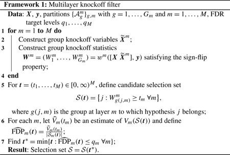
Constructing knockoffs for groups.

To carry out our layer-specific inference, we need to construct knockoffs for groups of variables.

Within the fixed design framework, we can rely on the recipe described in Dai and Barber (2016). These group knockoffs have the property that the first two sample moments of the augmented design matrix [$\mathit{X}\hspace{0.17em}{\tilde{\mathit{X}}}^m$] are invariant when any set of groups is swapped with their knockoffs. To be more precise, let ${\mathcal{C}}_m\subset [G_m]$ be a set of groups at the mth layer, and let

$$\mathcal{C}=\underset{g\in {\mathcal{C}}_m}{\cup }{\mathcal{A}}_g^m$$ (5)

be the variables belonging to any of these groups. Let ${[\mathit{X}\hspace{0.17em}{\tilde{\mathit{X}}}^m]}_{\text{swap(}\mathcal{C})}$ be the result of swapping the columns X_j and ${\tilde{\mathbf{X}}}_j$ in the augmented design matrix for each $j\in \mathcal{C}$. Invariance of empirical first moments to swapping can be achieved by centering all variables and their knockoffs, while invariance of empirical second moments requires that for each ${\mathcal{C}}_m$,

$${\left[\mathit{X}\hspace{0.17em}{\tilde{\mathit{X}}}^m\right]}_{\text{swap(}\mathcal{C})}^T{\left[\mathit{X}\hspace{0.17em}{\tilde{\mathit{X}}}^m\right]}_{\text{swap(}\mathcal{C})}={\left[\mathit{X}\hspace{0.17em}{\tilde{\mathit{X}}}^m\right]}^T\left[\mathit{X}\hspace{0.17em}{\tilde{\mathit{X}}}^m\right].$$ (6)

A construction of group knockoffs ${\tilde{\mathit{X}}}^m$ satisfying this property is given in Dai and Barber (2016). It is based on the observation that (6) is equivalent to

$$\begin{gathered} {\left({\tilde{\mathit{X}}}^m\right)}^T{\tilde{\mathit{X}}}^m=\mathbf{\Sigma }={\mathit{X}}^T\mathit{X};\hspace{1em}{\left({\tilde{\mathit{X}}}^m\right)}^T\mathit{X}={\mathbf{\Sigma }}^m-{\mathit{S}}^m; \\ \hspace{1em}\hspace{1em}{\mathit{S}}^m⪰0\hspace{0.17em}\text{group}\hspace{0.17em}\text{block}\hspace{0.17em}\text{diagonal}. \end{gathered}$$ (7)

For a fixed block diagonal matrix S^m, ${\tilde{\mathit{X}}}^m$ satisfying (7) can be constructed via

$${\tilde{\mathit{X}}}^m=\mathit{X}({\mathit{I}}_N-{\mathbf{\Sigma }}^{-1}{\mathit{S}}^m)+\tilde{\mathit{U}}{\mathit{C}}^m,$$

where $\tilde{\mathit{U}}$ is an n × N orthonormal matrix orthogonal to the span of X and C^m is a Cholesky square root of 2S^m – S^mΣ⁻¹S^m. The latter expression is positive semidefinite, if ${\mathit{S}}^m⪯\hspace{0.17em}2\mathbf{\Sigma }$. While there are several ways to construct ways to construct a block diagonal S^m satisfying $0⪯{\mathit{S}}^m⪯\hspace{0.17em}2\mathbf{\Sigma }$, the equicorrelated knockoff construction is defined via

$${\mathit{S}}^m=\text{diag}\left({\mathit{S}}_1^m,\hspace{0.17em}\dots \hspace{0.17em},{\mathit{S}}_{G_m}^m\right),\hspace{1em}\hspace{1em}{\mathit{S}}_g^m={\gamma }^m\cdot {\mathbf{\Sigma }}_{{\mathcal{A}}_g^m,{\mathcal{A}}_g^m},$$ (8)

where

$${\gamma }^m=\min \left(1,2\cdot {\lambda }_{\min }\left({\mathbf{D}}^m\mathbf{\Sigma }\hspace{0.17em}{\mathbf{D}}^m\right)\right)$$

and

$${\mathbf{D}}^m=\text{diag(}{\mathbf{\Sigma }}_{{\mathcal{A}}_1^m,{\mathcal{A}}_1^m}^{-1/2}\text{,}\hspace{0.17em}\dots \hspace{0.17em}\text{,}{\mathbf{\Sigma }}_{{\mathcal{A}}_{G_m}^m,{\mathcal{A}}_{G_m}^m}^{-1/2}).$$ (9)

Note that throughout this paper, all numerical experiments are based on the fixed design linear model and will thus use this construction.

Within the random design framework, the most natural way to define group knockoffs is to generalize the definition in Candès et al. (2018). For a set of random variables (X₁, X_N) and a set of groups ${\left\{{\mathcal{A}}_g^m\right\}}_{g\in [G_m]}$ a set of model-X group knockoffs $({\tilde{X}}_1^m,\hspace{0.17em}\dots \hspace{0.17em}{\tilde{X}}_N^m)$ is such that

$${(X_1,\hspace{0.17em}\dots \hspace{0.17em},X_N,{\tilde{X}}_1^m,\hspace{0.17em}\dots \hspace{0.17em},{\tilde{X}}_N^m)}_{\text{swap(}\mathcal{C})}\stackrel{d}{=}(X_1,\hspace{0.17em}\dots \hspace{0.17em},X_N,{\tilde{X}}_1^m,\hspace{0.17em}\dots \hspace{0.17em},{\tilde{X}}_N^m)$$ (10)

for any $\mathcal{C}$ of the form (5). Note that for regular model-X knockoffs, (10) must hold for all $\mathcal{C}$. Hence, less exchangeability is required of model-X group knockoffs which allows for them to be less similar to the original variables.

The sequential conditionally independent pairs (SCIP) procedure, proposed in Candès et al. (2018) to prove the existence of model-X knockoffs, generalizes straightforwardly to model-X group knockoffs. In particular the group SCIP procedure proceeds as follows: for each g = 1, …, G_m, we sample ${\tilde{X}}_{{\mathcal{A}}_g^m}^m$ from $\mathcal{L}(X_{{\mathcal{A}}_g^m}|X_{-{\mathcal{A}}_g^m},{\tilde{X}}_{{\mathcal{A}}_1^m,\hspace{0.17em}\dots \hspace{0.17em},{\mathcal{A}}_{g-1}^m}^m)$. The more explicit second-order knockoffs construction (exact for normally distributed variables) also carries over fairly directly. Suppose that X is distributed as N(0, Σ). Then, sampling

$${\tilde{X}}^m|X~N(\mathbf{\mu },\hspace{0.17em}\mathbf{V}),\hspace{1em}\mathbf{\mu }=X-X{\mathbf{\Sigma }}^{-1}{\mathit{S}}^m,\hspace{1em}\mathbf{V}=2{\mathit{S}}^m-{\mathit{S}}^m{\mathbf{\Sigma }}^{-1}{\mathit{S}}^m$$

yields a valid group model-X knockoff construction, where S^m is as defined in (8), (3.1) and (9). Note that X and μ are treated as row vectors of dimension 1 × N Recently, an HMM-based model-X knockoff construction has been proposed by Sesia, Sabatti and Candès (2019) tailored specifically for genetic design matrices. This construction can be generalized to the group setting as well [Matteo Sesia (2018), personal communication], though we do not discuss the details in the present work.

Constructing group importance statistics.

Once group knockoffs are constructed for each layer m, the next step is to define group importance statistics $({\mathit{Z}}^m,{\tilde{\mathit{Z}}}^m)=(Z_1^m,\hspace{0.17em}\dots \hspace{0.17em},Z_{G_m}^m,{\tilde{Z}}_1^m,\hspace{0.17em}\dots \hspace{0.17em},{\tilde{Z}}_{G_m}^m)=z^m\left(\left[\mathit{X}\hspace{0.17em}{\tilde{\mathit{X}}}^m\right],\mathit{y}\right)$, one for each group and each knockoff group. Here z^m is a function that assesses the association between each group (original and knockoff) and the response.

The function z^m must be group-swap equivariant, that is,

$$z^m({[\mathit{X}\hspace{0.17em}{\tilde{\mathit{X}}}^m]}_{\text{swap(}\mathcal{C})},y)={(Z_1^m,\hspace{0.17em}\dots \hspace{0.17em},Z_{G_m}^m,\hspace{0.17em}{\tilde{Z}}_1^m,\hspace{0.17em}\dots \hspace{0.17em},{\tilde{Z}}_{G_m}^m)}_{\text{swap}({\mathcal{C}}_m)}$$

for each ${\mathcal{C}}_m\subset [G_m]$ and corresponding $\mathcal{C}$ defined in (5). In words this means that swapping entire groups in [$\mathit{X}{\tilde{\mathit{X}}}^m$] translates to swapping the entries of (Z^m, ${\tilde{\mathit{Z}}}^m$) corresponding to those groups. For fixed design knockoffs, z^m must also satisfy the sufficiency property; z^m must operate on the data only through the sufficient statistics [$\mathit{X}{\tilde{\mathit{X}}}^m$]^T y and ${[\mathit{X}\hspace{0.17em}{\tilde{\mathit{X}}}^m]}^T[\mathit{X}\hspace{0.17em}{\tilde{\mathit{X}}}^m]$. Taken together, these steps lead to a function w^m mapping the augmented design matrix and response vector to a vector of knockoff statistics ${\mathbf{W}}^m=\left(W_1^m,\hspace{0.17em}\dots \hspace{0.17em},W_{G_m}^m\right)$.

There are many possible choices of z^m, and any choice satisfying group-swap equivariance (and sufficiency, for fixed design knockoffs) is valid. However, different choices will lead to procedures with different power. Generalizing the proposal of Dai and Barber (2016)—based on the group lasso—we consider a class of group importance statistics (Z^m, ${\tilde{\mathit{Z}}}^m$) obtained by first solving for each λ the penalized

$$\begin{gathered} {\mathit{b}}^{★}(\lambda ),{\tilde{\mathit{b}}}^{★}(\lambda )=\underset{\mathit{b},\tilde{\mathit{b}}}{\arg \min }\frac{1}{2}{\Vert \mathbf{y}-[\mathit{X}\hspace{0.17em}{\tilde{\mathit{X}}}^m]\left(\begin{array}{c}\mathit{b}\\ \tilde{\mathit{b}}\end{array}\right)\Vert }^2 \\ \hspace{1em}\hspace{1em}\hspace{1em}\hspace{1em}\hspace{1em}\hspace{1em}\hspace{1em}+\lambda \left(\sum _{g=1}^{G_m}{\mathcal{l}}_g^m({\mathit{b}}_{{\mathcal{A}}_g^m})+\sum _{g=1}^{G_m}{\mathcal{l}}_g^m({\tilde{\mathit{b}}}_{{\mathcal{A}}_g^m})\right), \end{gathered}$$ (11)

where ${\ell }_g^m$ are arbitrary penalty functions [the group lasso corresponds to ${\ell }_g^m(\mathit{u})=\sqrt{\left|{\mathcal{A}}_g^m\right|}{\Vert \mathit{u}\Vert }_2$]. The group importance statistics $Z_g^m({\tilde{Z}}_g^m)$ are then defined as the value of λ for which the group ${\mathit{X}}_{{\mathcal{A}}_g^m}({\tilde{\mathit{X}}}_{{\mathcal{A}}_g^m})$ first enters the lasso path:

$$Z_g^m=\sup \{\lambda :{\mathit{b}}_{{\mathcal{A}}_g^m}^{★}(\lambda )\ne 0\},\hspace{1em}\hspace{1em}{\tilde{Z}}_g^m=\sup \{\lambda :{\tilde{\mathit{b}}}_{{\mathcal{A}}_g^m}^{★}(\lambda )\ne 0\}.$$ (12)

For each m the regularization in (11) is defined on subsets of b corresponding to groups at the m layers, and it is separable with respect to the mth partition $\left\{{\mathcal{A}}_g^m\right\}$. While this guarantees group-swap equivariance and sufficiency, other constructions are certainly possible.

Different choices of ${\ell }_g^m$ allow us to adapt to the available information on signal structure and potentially gain power. The 2-norm defining the group lasso leads to entire groups entering the regularization path at the same time, so each variable in a group contributes equally to the corresponding group importance statistic. Drawing an analogy to global testing, this definition is similar to the Fisher combination test or the chi-squared test which are known to be powerful in regimes when the signal is weak and distributed. In our case, we should apply group lasso based statistics if we suspect that each group has many non-nulls. Taking this analogy further, we can also construct a Simes-like statistic that is more suited to the case when we believe each group has a few strong signals. This test statistic is defined by letting ${\ell }_g^m(\mathbf{u})={\Vert \mathbf{u}\Vert }_1$, that is, running a regular lasso regression. This will allow for each variable to come in on its own, and the knockoff statistic $W_g^m$ will be driven by the strongest predictor in the corresponding group.

Constructing group knockoff statistics.

Finally, group knockoff statistics are defined via $W_g^m=f_g^m(Z_g^m,{\tilde{Z}}_g^m)$, where $f_g^m$ is any antisymmetric function (i.e., swapping its arguments negates the output), such as the difference $f(Z_g^m,{\tilde{Z}}_g^m)=Z_g^m-{\tilde{Z}}_g^m$ or the signed-max $f(Z_g^m,{\tilde{Z}}_g^m)=\max (Z_g^m-{\tilde{Z}}_g^m)\cdot \mathrm{sgn}(Z_g^m-{\tilde{Z}}_g^m)$. Hence, $W_g^m$ quantifies the difference in how significantly associated ${\mathit{X}}_{{\mathcal{A}}_g^m}$ and ${\tilde{\mathit{X}}}_{{\mathcal{A}}_g^m}$ are with y.

Definition of ${\widehat{\mathit{V}}}_m(t_m)$. The FDR guarantee for the method depends crucially on the estimate ${\widehat{V}}_m(t_m)$ of $V_m(\mathcal{S}(t))$. Intuitively, the larger ${\widehat{V}}_m(t_m)$ is, the stronger the FDR guarantee. For the original knockoff filter [Barber and Candès (2015)], two choices of $\widehat{V}(t)$ were considered: $\widehat{V}(t)=\left|\{j:W_j\le -t\}\right|$(which leads to a procedure we abbreviate KF, for knockoff filter) and $\widehat{V}(t)=1+\left|\{j:W_j\le -t\}\right|$ (leading to a procedure we abbreviate KF+). Note that these are defined in terms of the size of the set obtained from $\mathcal{S}(t)=\{j:W_j\ge t\}$ by reflection about the origin. These definitions are motivated by the sign-flip property, and it can be easily shown that $\widehat{V}(t)=\left|\{j:W_j\le -t\}\right|$ is a conservative estimate for $V(\mathcal{S}(t))=\left|\{\text{null}\hspace{0.17em}j:W_j\ge t\}\right|$. The reason for also considering $\widehat{V}(t)=1+\left|\{j:W_j\le -t\}\right|$ is that the extra 1 is needed for exact FDR control. The KF procedure, defined without this extra 1, controls a weaker criterion called the mFDR, which is defined as follows:

$$\text{mFDR}=\mathbb{E}\left[\frac{\left|\mathcal{S}\cap {\mathcal{H}}_0\right|}{\left|\mathcal{S}\right|+q^{-1}}\right].$$

Similarly, we consider methods MKF and MKF+ based on two definitions of ${\widehat{V}}_m(t_m)$. However, we shall also consider the effect of adding a constant multiplier c to this estimate as well; see Procedures 1 and 2.

Procedure 1: MKF(c)

1 Framework 1, with ${\widehat{V}}_m(t_m)=c\cdot \left|\{g:W_g^m\le -t_m\}\right|$.

Procedure 2: MKF(c)+

1 Framework 1, with ${\widehat{V}}_m(t_m)=c\cdot (1+\left|\{g:W_g^m\le -t_m\}\right|)$.

Definition and computation of t^∗ Note that the last step in Framework 1 needs clarification, since the minimum of a set in M dimensions is not well defined in general. However, the following lemma resolves the issue.

Lemma 1. Consider the set of valid thresholds

$$\mathcal{T}=\mathcal{T}(q_1,\hspace{0.17em}\dots \hspace{0.17em},q_M)=\left\{\mathbf{t}:{\widehat{\text{FDP}}}_m(\mathbf{t})\le q_m\hspace{0.17em}for\hspace{0.17em}all\hspace{0.17em}m\right\}.$$ (13)

For any definition of ${\widehat{V}}_m(\cdot )$ in Framework 1 depending only on tm (as opposed to the entire vector t), the set $\mathcal{T}$ will possess the “lower left-hand corner property” which means that it contains the point ${\mathbf{t}}^{\ast }=\left(t_1^{\ast },\hspace{0.17em}\dots \hspace{0.17em},t_M^{\ast }\right)$ defined by

$$t_m^{\ast }=\min \left\{t_m:(t_1,\hspace{0.17em}\dots \hspace{0.17em},t_M)\in \mathcal{T}\hspace{0.17em}for\hspace{0.17em}some\hspace{0.17em}{t}_1,\hspace{0.17em}\dots \hspace{0.17em},t_{m-1},t_{m+1},\hspace{0.17em}\dots \hspace{0.17em},t_M\right\}.$$

Hence, the point t^∗ is the lower left-hand corner of $\mathcal{T}$ and is the minimum in the last step of Procedure 1. The p-filter enjoys this same property, and in fact the proof of this lemma is the same as that of Theorem 3 in Barber and Ramdas (2017). In addition to being well defined, the threshold t* can be computed efficiently using the same iterative coordinate-wise search algorithm proposed in Barber and Ramdas (2017).

Figure 2 provides an illustration of the multilayer knockoff filter on simulated data. The 2000 variables are broken into 200 groups, each of size 10. (More details about this example are in Section 4.1; it corresponds to the high saturation setting, with SNR = 0.5 and variable correlation 0.1.) The multilayer knockoff filter for the individual layer and the group layer results in the selection region in the upper right-hand corner and enjoys high power. For comparison the (single layer) knockoff filter selects all points to the right of the broken line; among these there are several nulls not selected by MKF as their group signal is not strong enough. In this simulation MKF reduces false positives without losing any power.

FIG. 2.

Illustration of one run of the multilayer knockoff filter. Each point represents an individual-layer hypothesis j with coordinates $W_j^1$ and $W_{g(j,2)}^2$ circles indicate nulls, asterisks non-nulls. The solid black lines are the thresholds for multilayer knockoff filter, while reflected gray lines are used in the definition of ${\widehat{V}}_m$. The broken black line represents the threshold for knockoff filter. The darkly shaded upper right corner represents the selection set of the multilayer knockoff filter, and the lightly shaded left half-plane represents the area used to define ${\widehat{V}}_{\text{ind}}$.

Computational complexity.

Computationally, both the multilayer knockoff filter and the original knockoff filter can be broken down into three distinct parts: constructing knockoff variables, computing knockoff statistics and then filtering those statistics to obtain a final selection set. Usually, the bottleneck is the second step; computing knockoff statistics involves solving a regularized regression of size n × 2N which costs O(nN²) (assuming for the moment n > 2N). Constructing knockoff variables, which for the genetic application at hand is best done using HMM knockoffs [Sesia, Sabatti and Candès (2019)], only costs O(nN). Finally, the filtering costs O(N). The same computational costs apply to the multilayer knockoff filter, except the first two steps must be done M times. In summary, the computational cost of the multilayer knockoff filter is equivalent to that of solving M regularized regressions. Solving regularized regressions is a standard computational task, and optimized solvers exist for these purposes such as glmnet [Friedman, Hastie and Tibshirani (2010)] or SparSNP [Abraham et al. (2012)], the former being general purpose and the latter being specialized for genetics applications. Indeed, the feasibility of knockoff analysis of GWAS data has been already illustrated in Candès et al. (2018) and Sesia, Sabatti and Candès (2019). Moreover, computations of the knockoff statistics for the M layers are independent and thus can be run in parallel, ensuring that the multilayer knockoff filter scales well to genome-wide data sets.

3.2. Theoretical guarantees.

Our main theoretical result guarantees that the MKF(c_kn)+ has multilayer FDR control at the target levels and that MKF(c_kn) has multilayer mFDR control at the target levels, where c_kn = 1.93.

Theorem 1. Suppose W^m obeys the sign-flip property for all m. Then, the MKF(c)+ method satisfies

$${\text{FDR}}_m\le \frac{c_{\text{kn}}}{c}{q}_m\hspace{1em}\hspace{1em}for\hspace{0.17em}all\hspace{0.17em}m,$$

where c_kn = 1.93. The MKF(c) method satisfies

$${\text{mFDR}}_m\le \frac{c_{\text{kn}}}{c}{q}_m\hspace{1em}\hspace{1em}for\hspace{0.17em}all\hspace{0.17em}m.$$

In particular, the MKF(c_kn)+ and MKF(c_kn) methods have multilayer FDR control and multilayer mFDR control, respectively, at the target levels.

While deferring technical lemmas to the Supplementary Materials [Katsevich and Sabatti (2018)], we outline here the essential steps of the proof as they differ fundamentally from those of KF and p-filter. The proof of FDR control for the knockoff filter relies on a clever martingale argument that depends heavily on the fact that the threshold t is one-dimensional; the cutoff t^∗ can be viewed as a stopping time with respect to a certain stochastic process. Instead, we are dealing with an M-dimensional threshold t^∗ whose entries depend on the values of W^m for all m. As the knockoff statistics have complex dependencies with each other, we cannot represent t_m as a stopping time with respect to a process that depends only on W^m. The p-filter being a multilayer method, the proof of FDR control deals with the complex nature of the threshold t^∗ However, by defining the p-values at each layer from the individual hypotheses p-values with a set rule, Barber and Ramdas (2017) have a good handle on the dependencies between $p_g^m$ across layers and use this crucially in the proof. In contrast we intentionally avoid specifying the relations between W^m for different m.

Proof. We prove FDR control for MKF(c)+; the result for MKF(c) follows from a very similar argument. We start introducing the following quantities:

$$V_m^{+}(t_m)=\left|\left\{g:W_g^m\ge t_m\right\}\cap {\mathcal{H}}_0^m\right|,\hspace{1em}\hspace{1em}{V}_m^{-}(t_m)=\left|\left\{g:W_g^m\le -t_m\right\}\cap {\mathcal{H}}_0^m\right|.$$

Note that both $V_m^{+}(t_m)$ and $V_m^{-}(t_m)$ are defined in terms of the mth layer only and that $\text{923966MC }$, while $V_m^{-}(t_m)$ is similar to ${\widehat{V}}_m(t_m)$. It is easy to verify that these two quantities satisfy

$$V_m^{+}(t_m)\ge V_m\left(\mathcal{S}(\mathbf{t})\right),\hspace{1em}\hspace{1em}{\widehat{V}}_m(t_m)\ge c\left(1+V_m^{-}(t_m)\right).$$

Then, for each m, we have

$$\begin{gathered} {\text{FDR}}_m=\mathbb{E}\left[{\text{FDR}}_m({\mathbf{t}}^{\ast })\right]=\mathbb{E}\left[\frac{V_m(\mathcal{S}({\mathbf{t}}^{\ast }))}{\left|\mathcal{S}({\mathbf{t}}^{\ast })\right|}\right] \\ \hspace{1em}\hspace{1em}\hspace{0.17em}\hspace{0.17em}\hspace{0.17em}=\mathbb{E}\left[\frac{V_m(\mathcal{S}({\mathbf{t}}^{\ast }))}{\left|\mathcal{S}({\mathbf{t}}^{\ast })\right|}I({\mathbf{t}}^{\ast }<\infty )\right] \\ \hspace{1em}\hspace{1em}\hspace{0.17em}\hspace{0.17em}\hspace{0.17em}=\mathbb{E}\left[\frac{V_m(\mathcal{S}({\mathbf{t}}^{\ast }))}{{\widehat{V}}_m(t_m^{\ast })}\frac{{\widehat{V}}_m(t_m^{\ast })}{\left|{\mathcal{S}}_m({\mathbf{t}}^{\ast })\right|}I({\mathbf{t}}^{\ast }<\infty )\right] \\ \hspace{1em}\hspace{1em}\hspace{0.17em}\hspace{0.17em}\hspace{0.17em}\le q_m\cdot \frac{1}{c}\mathbb{E}\left[\frac{V_m^{+}(t_m^{\ast })}{1+V_m^{-}(t_m^{\ast })}\right] \\ \hspace{1em}\hspace{1em}\hspace{0.17em}\hspace{0.17em}\hspace{0.17em}\le q_m\cdot \frac{1}{c}\mathbb{E}\left[\underset{t_m}{\sup }\frac{V_m^{+}(t_m^{\ast })}{1+V_m^{-}(t_m^{\ast })}\right]. \end{gathered}$$ (14)

Hence it suffices to show that

$$\mathbb{E}\left[\underset{t_m\ge 0}{\sup }\frac{V_m^{+}(t_m)}{1+V_m^{-}(t_m)}\right]\le c_{\text{kn}}.$$ (15)

The introduction of the supremum over t_m in the last equation is a key step in the proof. It makes the random variables in the expectation (15) depend only on the knockoff statistics at the mth layer, decoupling the problem across layers and allowing any type of dependence between statistics for different values of m.

Given that we are working with quantities defined in one layer only, we can drop the subscript m and consider (15) as a statement about any set of knockoff statistics (W₁, …, W_G) satisfying the sign-flip property. Hence, $W_g^m$, $V_m^{+}(t_m)$, $V_m^{-}(t_m)$ become W_g, V⁺(t), V⁻(t), respectively, and so on. We are left with

$$\begin{gathered} \mathbb{E}\left[\underset{t\ge 0}{\sup }\frac{V^{+}(t)}{1+V^{-}(t)}\right]=\mathbb{E}\left[\underset{t\ge 0}{\sup }\frac{\left|\{g:W_g\ge t\}\cap {\mathcal{H}}_0\right|}{1+\left|\{g:W_g\le -t\}\cap {\mathcal{H}}_0\right|}\right] \\ \hspace{1em}\hspace{1em}\hspace{1em}\hspace{1em}\hspace{1em}\hspace{1em}\hspace{0.17em}\hspace{0.17em}=\mathbb{E}\left[\mathbb{E}\left[\underset{t\ge 0}{\sup }\frac{\left|\{g:W_g\ge t\}\cap {\mathcal{H}}_0\right|}{1+\left|\{g:W_g\le -t\}\cap {\mathcal{H}}_0\right|}\right|\left|\mathbf{W}\right|\right]]. \end{gathered}$$ (16)

Now, consider ordering ${\left\{W_g\right\}}_{g\in {\mathcal{H}}_0}$ by magnitude:$\left|W_{(1)}\right|\ge \hspace{0.17em}\dots \hspace{0.17em}\ge \left|W_{(G_0)}\right|$, where $G_0=\left|{\mathcal{H}}_0\right|$. Let σ_g = sgn(W_(g)). By the sign-flip property σ_g are distributed as i.i.d. coin flips independently of |W|. Moreover, note that the quantity inside the expectation is constant for all t except $t\in \left\{\left|W_{(1)}\right|\ge \hspace{0.17em}\dots \hspace{0.17em}\ge \left|W_{(G)}\right|\right\}$, and for t = |W_(k)|, we have

$$\begin{gathered} \frac{\left|\{g:W_g\ge t\}\cap {\mathcal{H}}_0\right|}{1+\left|\{g:W_g\le -t\}\cap {\mathcal{H}}_0\right|}=\frac{\left|\{g:W_g\ge \left|W_{(k)}\right|\}\cap {\mathcal{H}}_0\right|}{1+\left|\{g:W_g\le -\left|W_{(k)}\right|\}\cap {\mathcal{H}}_0\right|} \\ \hspace{1em}\hspace{1em}\hspace{1em}\hspace{1em}\hspace{1em}\hspace{1em}=\frac{\left|\{g\le k:{\sigma }_j=+1\right|}{1+\left|\{g\le k:{\sigma }_j=-1\right|}. \end{gathered}$$

Putting these pieces together, we have

$$\mathbb{E}\left[\underset{t\ge 0}{\sup }\frac{V^{+}(t)}{1+V^{-}(t)}\right]=\mathbb{E}\left[\underset{k\le G_0}{\max }\frac{\left|\{g\le k:{\sigma }_g=+1\}\right|}{1+\left|\{g\le k:{\sigma }_g=-1\}\right|}\right].$$

We can think of σ_g as the increments of a simple symmetric random walk on $\mathbb{Z}$. The numerator above represents the number of steps to the right this walk takes, and the denominator the number of steps to the left. The quantity we are bounding is essentially the maximum over all steps in the walk of the ratio of steps right to steps left, averaged over all realizations of the random walk. Let S_k = |{g ≤ k : σ_g = +1}| be the number of steps right and k − S_k = |{g ≤ k σ_g = −1}| the number of steps left. It suffices to show that

$$\mathbb{E}\left[\underset{k\ge 0}{\sup }\frac{S_k}{1+k-S_k}\right]\le \mathrm{1.93.}$$ (17)

This is the content of Lemma 3, which is proved in the Supplementary Material [Katsevich and Sabatti (2018)]. □

3.3. Relations with other methods.

Comparison to other structured testing methods.

When scientific hypotheses have a complex structure, even formulating inferential guarantees is nontrivial; the multilayer hypothesis testing approach proposed in Barber and Ramdas (2017) and used in our work is one of several options. Approaches to testing hypotheses at multiple levels vary in two key features: the way the space of hypotheses is traversed and the way families to be tested are defined. We illustrate the different approaches using the two-layer setup considered in the Introduction. If the hypotheses have a nested (i.e., tree) structure, then it is common to traverse them hierarchically; one starts by testing groups and then proceeds to test individual hypotheses within rejected groups. The procedures described in Benjamini and Bogomolov (2014), Bogomolov et al. (2017), Yekutieli (2008) follow this hierarchical approach. An alternative to hierarchical hypothesis traversal is to consider the multiple testing problem from the point of view of individual-level hypotheses. Rejecting a set of individual-level hypotheses induces the rejections of the groups that contain them at each layer of interest. This is the approach taken by the p-filter [Barber and Ramdas (2017)]. By testing hypotheses only if their corresponding groups were rejected, hierarchical approaches have the advantage of a smaller multiplicity burden. On the other hand, defining selections at each layer via the individual-level hypotheses has the advantage that it applies equally well to non-hierarchical ways of grouping hypotheses. The second dichotomy in based on how one defines families to be tested. Either each group is a family of its own, or each resolution is a family of its own. For instance, the former corresponds to SNPs being tested against other SNPs in the same gene, and the latter corresponds to testing all SNPs against each other as one family. The methods of Benjamini and Bogomolov (2014) and Bogomolov et al. (2017) take the former approach, while those of Yekutieli (2008) and Barber and Ramdas (2017) take the latter. Both choices can be meaningful, depending on the application. In this work, we define discoveries using individual-level hypotheses as this marries well with the multiple regression framework and does not limit us to nested groups. We treat each resolution (instead of each group) as a family because discoveries are often reported by type (e.g., as a list of SNPs or a list of genes), so FDR guarantees for each type are appropriate. These two choices align our testing framework with that of the p-filter.

The multiplier c_kn: Its origins and impact.

In addition to using knockoff statistics instead of p-values, the multilayer knockoff filter differs from the p-filter [Barber and Ramdas (2017)] in that it does not start from a set of individual-level statistics and construct group-level ones using specific functions of these. Instead the statistics W^m are constructed starting directly from the original data. This decision involves a trade-off; we get a more general procedure (and theoretical result) at the cost of a looser bound.

By making no assumptions on the between-layer dependencies of $W_g^m$, the multilayer knockoff filter allows extra flexibility that can translate into greater power. For example, there might be different sources of prior information at the SNP and the gene levels. The analyst can use each source of information at its respective layer to define more powerful knockoff statistics (based on specific penalties) without worrying about coordinating these statistics in any way. Even if the same penalization is used in all layers, there is a potential power increase due to the fact that we can use group knockoff variables rather than individual ones. This advantage is especially pronounced if none of the layers consists of singletons.

The price we pay for this generality is the multiplier c_kn = 1.93 in Theorem 1. To understand its effect, note that in Procedures 4 and 5, by analogy with KF, the natural choice is c = 1 and define MKF = MKF(1) and MKF+ = MKF(1)+. Then Theorem 1 states that MKF+ (MKF) has an FDR (mFDR) that is bounded by c_knq_m. Compare this to the theoretical result for the p-filter, which is shown to have exact multilayer FDR control, by explicitly leveraging the joint distribution of $p_g^m$; Barber and Ramdas (2017) get a handle on the complicated thresholds $t_m^{\ast }$ and get a tight result. Meanwhile, our constant multiplier comes from the introduction of the supremum in (14); this amounts to a worst-case analysis which for most constructions of $W_g^m$ will not be tight.

Indeed, across all our simulations in Section 4, we find that MKF+ has multilayer FDR control at the target levels (i.e., the constant is not necessary). Hence, we recommend that practitioners apply the MKF or MKF+ methods without worrying about the correction constants. We view our theoretical result as an assurance that even in the worst case, the FDRs of MKF at each layer will not be much higher than their nominal levels q_m.

Generalized p-filter.

On the heels of the above discussion, we define the generalized p-filter, a procedure that is the same as the p-filter, except that the p-values $p_g^m$ are any valid p-values for the hypotheses in layer m.

Theorem 2. Suppose for each m, the null p-values among $\left\{p_g^m\right\}$ are independent and uniformly distributed. Then, the generalized p-filter satisfies

$${\text{mFDR}}_m\le c_{\text{pf}}(G_m)\cdot q_m\hspace{1em}\hspace{1em}for\hspace{0.17em}all\hspace{0.17em}m,$$

where $c_{\text{pf}}(G)=1+\exp \left(G^{-1/2}+\frac{1}{2}{G}^{-1}\right)0.42+e{G}^{-1/4}$.

Remark 3.1. Unlike for the multilayer knockoff filter, note that we do not have one universal constant multiplier c_pf. Instead, we get a bound c_pf(G_m) that depends on the number of groups at each layer. However, strong numerical evidence suggests that in fact we can replace c_pf(G_m) in the theorem with its limiting value 1.42. See Remark C.1 in the Supplementary Material [Katsevich and Sabatti (2018)] for additional comments. Moreover, the assumption of independent null p-values can potentially be relaxed to a PRDS assumption, but we have not explored this avenue.

Proof. By similar logic as in the proof of Theorem 1, it suffices to verify the sufficient condition

$$\mathbb{E}\left[\underset{t_m\in [0,1]}{\sup }\frac{\left|\{g\in {\mathcal{H}}_0^m:p_g^m\le t_m\}\right|}{1+G_m{t}_m}\right]\le c_{\text{pf}}(G_m).$$

Again, note that the problem decouples across layers, and we may drop the subscript m. Now, let p₁, …, p_G be a sequence of i.i.d. uniform random variables, and let F_G(t) be their empirical CDF. Then, it suffices to show that

$$\mathbb{E}\left[\underset{t\in [0.1]}{\sup }\frac{F_G(t)}{G^{-1}+t}\right]\le 1+\exp \left(G^{-1/2}+\frac{1}{2}{G}^{-1}\right)0.42+e{G}^{-1/4}.$$

This is the content of Lemma 4 which is proved in the Supplementary Material [Katsevich and Sabatti (2018)]. □

Recently [Ramdas et al. (2017)], the p-filter methodology has been generalized to allow for more general constructions of group p-values but must use reshaping [a generalization of the correction proposed by Benjamini and Yekutieli (2001)] to guarantee FDR control. Hence, both generalizations must pay for arbitrary between-layer dependencies—our method with the constant c_pf and the p-filter with reshaping.

Power of multilayer methods.

By construction, the multilayer algorithms we propose are at most as powerful as their single-layer versions. For our purposes groups of variables function as inferential units, and not as prior information used to boost power [e.g., as in Li and Barber (2016)], although there is no reason groups cannot serve both functions within our framework. So while our methods are designed to provide more FDR guarantees, it is relevant to evaluate the cost in terms of power of these additional guarantees.

Consider controlling FDR for individual variables and for groups, compared to just controlling FDR for individual variables. When adding a group FDR guarantee, power loss depends on the group signal strength, the power of group statistics and the desired group FDR control level q_grp. Power will decrease to the extent that the signal strength at the group layer is weaker than the signal strength at the individual layer. Assuming for simplicity that non-null variables have comparable effect sizes, group signal is weak when saturation is low (recall from the Introduction that saturation is the average number of non-null variables per non-null group). Also, if the sizes of the groups vary, then group signal will be weaker if the non-null hypotheses are buried inside very large groups. Even if group signal is not too weak, the power of multilayer procedures will depend on the way group statistics are chosen. In particular, power will be better if Simes (or Simes-like) statistics are used if groups have a small number of strong signals, and if Fisher (or Fisher-like) statistics are used in the case of weak distributed effects. Finally, it is clear that lowering q_grp will lower power.

As a final note, all of the multilayer methods discussed so far have a feature that might unnecessarily limit their power. This feature is the definition of ${\widehat{V}}_m={\widehat{V}}_m(t_m)$ in terms of only the threshold t_m. Since the selection set $\mathcal{S}(\mathbf{t})$ is defined with respect to the M-dimensional vector of thresholds t, a definition of ${\widehat{V}}_m$ depending on this entire vector would be a better estimate of $V_m(\mathcal{S}(\mathbf{t}))$. In some situations the procedures proposed might overestimate $V_m(\mathcal{S}(\mathbf{t}))$ and thus pay a price in power. For a graphical illustration of this phenomenon, we revisit Figure 2. Note that we are using the number of points in the entire shaded left half-plane to estimate the number of false positives in just the shaded upper right quadrant. Unfortunately, this issue is not very easy to resolve. One challenge is that if we allow ${\widehat{V}}_m$ to depend on the entire vector t, then the definition of t* would be complicated by the fact that the lower left-hand corner property would no longer hold. Another challenge is that the dependencies between statistics across layers make it hard to come up with a better and yet tractable estimate of $V_m(\mathcal{S}(\mathbf{t}))$. Despite this flaw, the multilayer knockoff filter (and the p-filter) enjoys very similar power to its single-layer counterpart, as we shall see in the next section.

4. Simulations.

We rely on simulations to explore the FDR control and the power of the multilayer knockoff filter and the generalized p-filter across a range of scenarios, designed to capture the variability described in the previous section. All code is available at http://web.stanford.edu/~ekatsevi/software.html.

4.1. Performance of the multilayer knockoff filter.

Simulation setup.

We simulate data from the linear model with n > N This also allows us to calculate p-values for the null hypotheses β_j = 0 and plug these into BH and p-filter; these two methods, in addition to KF, serve as points of comparison to MKF.

We simulate

$$\mathit{y}=\mathit{X}\mathit{\beta }+\mathbf{\epsilon },\hspace{1em}\hspace{1em}\mathbf{\epsilon }~\mathcal{N}(0,\hspace{0.17em}\mathit{I}),$$

where $\mathit{X}\in {ℝ}^{n\times N}$ with n = 4500 observations on N = 2000 predictors. X is constructed by sampling each row independently from N(0, Σ_ρ), where ${({\mathbf{\Sigma }}_{\rho })}_{ij}={\rho }^{\left|i-j\right|}$ is the covariance matrix of an AR(1) process with correlation ρ. There are M = 2 layers: one comprising individual variables and one with G = 200 groups, each of 10 variables. The vector β has 75 nonzero entries. The indices of the non-null elements are determined by firstly selecting k groups uniformly at random, and then choosing, again uniformly at random, 75 elements of these k groups. Here, k controls the strength of the group signal. We considered three values: low saturation (k = 40), medium saturation (k = 20) and high saturation (k = 10). We generated these three sparsity patterns of β once and fixed them across all simulations; see Figure 3. In all cases the nonzero entries of β are all equal, with a magnitude that satisfies

$$\text{SNR=}\frac{{\Vert \mathit{X}\beta \Vert }^2}{n}$$

for a given SNR value. For each saturation setting we vary ρ ∈ {0.1, 0.3, …, 0.9} while keeping SNR fixed at 0.5 and vary SNR ∈ {0, 0.1, …, 0.5} while keeping ρ fixed at 0.3. Across all experiments we used nominal FDR levels q_ind = q_grp = 0.2.

FIG. 3.

Simulated sparsity patterns for the three saturation regimes. Each square corresponds to one variable, and each column to one group. Non-null variables are indicated with filled squares.

This choice of simulation parameters captures some of the features of genetic data. The AR(1) process for the rows of X is a first approximation for the local spatial correlations of genotypes, and the signal is relatively sparse, as we would expect in GWAS. A notable difference between our simulations and common genetic data is the scale; a typical GWAS involves N ≈ 1,000,000 variables. Previous studies [Candès et al. (2018), Sesia, Sabatti and Candès (2019)] have already demonstrated the feasibility of knockoffs for datasets of this scale, and the MKF does not appreciably differ in computational requirements. However, given our interest in exploring a variety of sparsity and saturation regimes, we found it convenient to rely on a smaller scale. Moreover, working in a regime where n > 2N allows us to leverage the fixed design construction of knockoff variables, which does not require knowledge of the distribution of X.

Methods compared.

We compare the following four methods on this simulated data:

1. KF+ with fixed design knockoffs, lasso-based variable importance statistics combined using the signed-max function, targeting q_ind.

2. MKF+ with fixed design group knockoffs, “Simes-like” group importance statistics based on the penalty ${\ell }_g^m(\mathbf{u})={\Vert \mathbf{u}\Vert }_1$, combined using the signed-max function, targeting q_ind and q_grp. We find that this choice of penalty has better power across a range of saturation levels than the group lasso based construction of Dai and Barber (2016).

3. Benjamini Hochberg procedure (BH) on the p-values based on t-statistics from linear regression, targeting q_ind.

4. p-filter (PF) on the same set of p-values, targeting q_ind and q_grp.

Note that the first two methods are knockoff based, the last two are p-value based and that methods (a) and (c) target only the FDR at the individual layer while methods (b) and (d) target the FDR at both layers.

Results.

Figure 4 illustrates our findings. First, consider the FDR of the four methods. The multilayer knockoff filter achieves multilayer FDR control across all parameter settings; the constant c_kn = 1.93 from our proof does not appear to play a significant role in practice. The p-filter also has multilayer FDR control, even though the PRDS assumption is not satisfied by the two-sided p-values we are using. On the other hand, the knockoff filter and BH both violate FDR control at the group layer as the saturation level and power increase.

FIG. 4.

Simulation results. From left to right, the saturation regime changes. The top panel varies signal-to-noise ratio while fixing ρ = 0.3. The bottom panel varies ρ while fixing SNR = 0.5. Each point represents the average of 50 experiments.

We also note that both the multilayer knockoff filter and regular knockoff filter have, on average, a realized FDP that is smaller than the target FDR. This is partly because we use the “knockoffs+” version of these methods which is conservative when the power is low. In addition we find that the multilayer knockoff filter is conservative at the individual layer even in high-power situations if the saturation is high. This is a consequence of our construction of ${\widehat{V}}_m$, an estimate of the number of false discoveries that, as we have discussed, tends to be larger than needed. We see similar behavior for the p-filter, since it has an analogous construction of ${\widehat{V}}_m$.

Next, we compare the power of the four methods. As expected, the power of all methods improves with SNR and degrades with ρ. We find that the knockoff-based approaches consistently outperform the p-value based approaches with higher power despite having lower FDRs and the gap widening as saturation increases. This power difference is likely caused by the ability of the knockoff-based approaches to leverage the sparsity of the problem to construct more powerful test statistics for each variable. Finally, we compare the power of the multilayer knockoff filter to that of the regular knockoff filter. In most cases the multilayer knockoff filter loses little or no power, despite providing an additional FDR guarantee. This holds even in the low saturation setting, where the groups are not very informative for the signal.

4.2. Performance of the generalized p-filter.

We explore the possible advantages of the generalized p-filter in a setup when signals are expected to be weak and common within non-null groups, so one would want to define group p-values via the Fisher test instead of the Simes test. We consider two partitions of interest, both with groups of size 10 (thus no singleton layer). A situation similar to this might arise when scientists are interested in determining which functional genomic segments are associated with a trait. There exist several algorithms to split the genome into functional blocks [e.g., ChromHMM by Ernst and Kellis (2012)], and segments in each of these can be partially overlapping.

Simulation setup.

We simulated N = 2000 hypotheses, with M = 2 layers. Each layer had 200 groups, each of size 10. The groups in the second layer were offset from the those in the first layer by five. Hence, the groups for layer one are {1, …, 10}, {11, …, 20}, while the groups for layer two are {6, …, 15}, {16, …, 25}, The nonzero entries of β are {1, …, 200}. Hence, this is a “fully saturated” configuration. We generate $X_j\stackrel{\text{ind}}{~}\mathcal{N}({\mu }_j,\hspace{0.17em}1)$, where μ_j = 0 for null j and μ_j = μ for non-null j We then derive two-sided p-values based on the z test. In this context, we define $\text{SNR}={\Vert \mu \Vert }^2/N$. The SNR varied in the range {0, 0.1, …, 0.5}, and we targeted q_ind = q_grp = 0.2.

Methods compared.

(a) The regular p-filter, which is based on the Simes test. (b) The generalized p-filter with p-values based on the Fisher test.

Results.

Figure 5 shows how both versions of the generalized p-filter have multilayer FDR control, with the Fisher version being more conservative. As with the multilayer knockoff filter, we see that the extra theoretical multiplicative factor is not necessary (at least in this simulation). In this case Fisher has substantially higher power than Simes due to the weak distributed effects in each group.

FIG. 5.

Performance of the generalized p-filter: comparison of Fisher and Simes combination rules.

5. Case study: Variants and genes influencing HDL.

To understand which genes are involved in determining cholesterol levels and which genetic variants have an impact on its value, Service et al. (2014) carried out exome resequencing of 17 genetic loci identified in previous GWAS studies as linked to metabolic traits in about 5000 subjects. The original analysis is based on marginal tests for common variants and burden tests for the cumulative effect of the rare variants in a gene [Li and Li (2008), Wu et al. (2011)]. Furthermore, to account for linkage disequilibrium and to estimate the number of variants that influence cholesterol in each location, Service et al. (2014) uses model selection based on BIC. The original analysis, therefore, reports findings at the gene level and variant level, but these findings derive from multiple separate analyses and lack coordination. Here we deploy MKF to leverage multiple regression models, obtaining a coherent set of findings at both the variant and gene level with approximate multilayer FDR control.

Data.

The resequencing targeted the coding portion of 17 genetic loci, distributed over 10 chromosomes and containing 79 genes. This resulted in the identification of a total of 1304 variants. We preprocessed the data as in Stell and Sabatti (2016), who reanalyzed the data in a Bayesian framework. In particular, we removed variants with minor allele counts below a threshold and pruned the set of polymorphisms to assure that the empirical correlation between any pair is of at most 0.3 [this is a necessary step in multiple regression analysis to avoid collinearity; see Brzyski et al. (2017) and Candès et al. (2018)]. After preprocessing, the data contained 5335 individuals and 768 variants. Since the study design was exome resequencing, every variant could be assigned to a gene. A special case is that of 18 SNPs that were typed in a previous study of these subjects and that were included in the final analysis as indicators of the original association signal; 12 of these are located in coding regions, but six are not.

While Service et al. (2014) studies the genetic basis of several metabolic traits, we focus our analysis here on HDL cholesterol. From the original measurement we regressed out the effects of sex, age and the first five principal components of genomewide genotypes representing population structure.

Note that the small size of the dataset is due to the design of the study, which relies on targeted resequencing as opposed to an exome-wide or genome-wide resequencing. Working with a small set of variables that have been quite extensively analyzed already allows us to better evaluate the MKF results, which is useful in a first application. The analysis with MKF of a new exome-wide data set comprising tens of thousands of individuals and hundreds of thousands of variants is ongoing.

Methods compared.

To focus on the effect of adding multilayer FDR guarantees (rather than on the consequences of different methods of analysis), we compare the results of the multilayer knockoff filter (MKF) and the knockoff filter (KF). The multilayer knockoff filter used a variant layer and a gene layer. We chose MKF and KF instead of MKF+ and KF+ for increased power but otherwise used the same method settings as in Section 4. Each variant from the sequencing data and the 12 exonic GWAS SNPs were assigned to groups based on gene. The six intergenic GWAS SNPs are considered single members of six additional groups. Hence, our analysis has 85 (= 79 + 6) “genes” in total.

Results.

Table 1 summarizes how many genes and SNPs each method discovers. KF has about twice as many discoveries at each layer, but how many of these are spurious? Unfortunately, the identity of the variants truly associated with HDL is unknown, but we can get an approximation to the truth using the existing literature and online databases. At the variant level, this task is difficult because (1) linkage disequilibrium (i.e., correlations between nearby variants) makes the problem ill-posed and (2) rare variants, present in this sequencing dataset, are less well studied and cataloged. Instead, we focus on an annotation at the gene level. Comparing the two methods at the gene level is also meaningful because this is the layer at which the multilayer knockoff filter provides an extra FDR guarantee. See Appendix D for references supporting our annotations.

TABLE 1.

Summary of association results on resequencing data

Method	# SNPs found	# genes found
KF	23	11
MKF	13	6

Table 2 shows the gene layer results: there are five true positive genes (ABCA1, CETP, GALNT2, LIPC, LPL) found by both methods, one false positive shared by both methods (PTPRJ), one true positive for KF that is missed by MKF (APOA5) and four false positives (NLRC5, SLC12A3, DYNC2LI1, SPI1) for KF that MKF correctly does not select. Hence, MKF reduced the number of false positives from five to one at the cost of one false negative.

TABLE 2.

Comparison of MKF and KF at the gene layer. False positives are highlighted in italics

Gene	Discovered by	Supported in literature
ABCA1	KF, MKF	Yes
CETP	KF, MKF	Yes
GALNT2	KF, MKF	Yes
LIPC	KF, MKF	Yes
LPL	KF, MKF	Yes
PTPRJ	KF, MKF	No
APOA5	KF	Yes
NLRC5	KF	No
SLC12A3	KF	No
DYNC2LI1	KF	No
SPI1	KF	No

Figure 6 shows a more detailed version of these association results, illustrating the signal at the variant level. Notably, the one extra false negative (APOA5) incurred by MKF just barely misses the cutoff for the gene layer. Aside from the extra false negative and the one false positive shared with KF, the additional horizontal cutoff induced by the need to control FDR at the gene level does a good job separating the genes associated with HDL from those that are not.

FIG. 6.

Scatterplot of variant level and gene level knockoff statistics. Solid blue lines are the thresholds for MKF while the cyan broken line is the threshold for KF. Each dot corresponds to a variant, and variants selected by at least one of the methods are in color: dark green indicates selected variants that belong to genes that are true positives for both methods, light green a true positive found by KF but missed by MKF, red is for false positives of KF but true negatives of MKF and magenta for the false positive shared by both methods. To facilitate comparison with Table 2, we indicate the names of the genes representing false positives or false negatives for at least one of the methods.

6. Conclusions.

With the multilayer knockoff filter, we have made a first step to equip model selection procedures with FDR guarantees for multiple types of reported discoveries. This bridges results from the multiresolution testing literature [Barber and Ramdas (2017), Benjamini and Bogomolov (2014), Peterson et al. (2016), Yekutieli (2008)] with controlled selection methods [Barber and Candès (2015), Candès et al. (2018), Dai and Barber (2016)]. When tackling high dimensional variable selection, researchers have at their disposal several methods based on regularized regression with penalties that can reflect an array of sparse structures [see, e.g., Jalali et al. (2010), Kim and Xing (2009), Rao et al. (2013)], corresponding to a multiplicity of possible resolutions for discoveries. While several of them have been implemented in the context of genetic association studies [Xing et al. (2014), Zhou et al. (2010)], their application has been hampered by the lack of inferential guarantees on the selection. It is our hope that the approach put forward with MKF will allow scientists to leverage these computationally attractive methods to obtain replicable discoveries at multiple levels of granularity.

In the process of developing a framework for multilayer FDR control for variable selection, we have also generalized the p-filter multiple testing procedure. Our approach places no restrictions on the relations between the p-values used to test the hypotheses at different layers. By contrast theoretical results for the p-filter rely heavily on the specific way in which p-values for individual hypotheses are aggregated to obtain p-values for groups. The constant c_pf can be viewed as the price we pay for allowing these arbitrary dependencies. Nevertheless, simulations show that both c_pf and the corresponding constant c_kn for MKF appear to be inconsequential in practice.

Finally, the uniform bound (15) can be reinterpreted as stating that the maximum amount by which the FDP of the knockoff filter can exceed $\widehat{\text{FDP}}$ over the entire path has bounded expectation. Moreover, the same proof yields a high-probability uniform bound on FDP. This interpretation is pursued by Katsevich and Ramdas (2018), who also prove the corresponding bound for BH conjectured here and extend the proof to a variety of other FDR methodologies.

Extensions.

There are many directions, of varying degrees of difficulty, in which it seems appropriate to extend the results we have so far. We list some below.

We have constructed the multilayer framework so that it would not require the groups in different layers to be hierarchically nested. However, in certain applications, such a hierarchical structure exists and could be exploited to increase power, relaxing the consistency requirements we have for discoveries across layers. This is the case, for example, in the relation between SNPs and genes that partially motivated us. It is scientifically interesting to discover that a gene is implicated in a disease, even if we are unable to pinpoint any specific causal variant within that gene. Formally, the selection sets allowed in this paper at each layer must be “two-way consistent,” that is, selecting an individual variable implies selecting the group to which it belongs, and selecting a group implies selecting at least one variable in the group. In a hierarchical setting a less stringent “one-way consistency” requirement can be formulated; selecting an individual variable implies selecting the group to which it belongs. In fact it can be easily shown that MKF can be modified to enforce this relaxed consistency requirement, and the same proof technique shows that multilayer FDR control still holds. This modified MKF is currently being used to analyze data from an exome-wide resequencing study.

In the genetic application motivating this work, SNPs are grouped according to the genes to which they belong. This is adequately described with nonoverlapping groups, but there are extensions in which it makes sense to consider groups that are overlapping within the same layer. For example, biological pathways are groups of genes known to work together to carry out a certain biological function. It is often desired for inference to be carried out at the pathway level, as this gives a direct biological interpretation of the results. However, genes often participate in multiple pathways, which leads to large group overlaps. This brings new statistical challenges, starting from a meaningful description of the null hypothesis for each group, to the construction of valid knockoff variables for overlapping groups.

We have focused on situations where the researcher, prior to looking at the data, can specify meaningful groups of variables corresponding to discoveries at coarser resolutions. While this is the case in many settings where it makes sense to pursue FDR control at multiple layers, it is also true that there are problems where the groupings of predictors are most meaningful when based on the data. For example, in our own case study, we grouped predictors as individual variables that are too correlated with each other. While we did so in a fairly arbitrary manner and without looking at the outcome variable, choosing groups based on the data could have helped us to choose a “resolution” appropriate for the signal strength and correlation structure in the data. Even in a single-layer setup, selecting groups and then carrying out valid inference with respect to these groups is a challenging new problem; we hope that some of the ideas developed here can contribute to its solution.

Another promising extension of the MKF is to multitask regression, the study of the impact of a set of predictor variables on multiple outcome variables. The multitask regression problem is often reshaped into a larger single-task regression problem in which the predictors have group structure based on the task to which they correspond. For example, Dai and Barber (2016) take this approach to multitask regression alongside its development of the group knockoff filter. MKF can then provide a framework for FDR control in this setting, where group discoveries correspond to finding variables important for at least one of the outcomes, and individual discoveries correspond to the identification of variables important for a specific outcome. In the context of the linear model with N ≤ n and independent errors, the MKF as described here provides the desired FDR guarantee. However, the general case is more challenging and will require substantial modifications.

REFERENCES

- ABRAHAM G, KOWALCZYK A, ZOBEL J and INOUYE M (2012). SparSNP: Fast and memory-efficient analysis of all SNPs for phenotype prediction. BMC Bioinform 13 Art. ID 88. [DOI] [PMC free article] [PubMed] [Google Scholar]
- BARBER RF and CANDÈS EJ (2015). Controlling the false discovery rate via knockoffs. Ann. Statist 43 2055–2085. MR3375876 [Google Scholar]
- BARBER RF and RAMDAS A (2017). The p-filter: Multilayer false discovery rate control for grouped hypotheses. J. Roy. Statist. Soc. Ser. B 79 1247–1268. MR3689317 [Google Scholar]
- BENJAMINI Y and BOGOMOLOV M (2014). Selective inference on multiple families of hypotheses. J. Roy. Statist. Soc. Ser. B 76 297–318. MR3153943 [Google Scholar]
- BENJAMINI Y and HELLER R (2007). False discovery rates for spatial signals. J. Amer. Statist. Assoc 102 1272–1281. MR2412549 [Google Scholar]
- BENJAMINI Y and HOCHBERG Y (1995). Controlling the false discovery rate: A practical and powerful approach to multiple testing. J. Roy. Statist. Soc. Ser. B 57 289–300. MR1325392 [Google Scholar]
- BENJAMINI Y and YEKUTIELI D (2001). The control of the false discovery rate in multiple testing under dependency. Ann. Statist 29 1165–1188. MR1869245 [Google Scholar]
- BOGDAN M, VAN DEN BERG E, SABATTI C, SU W and CANDÈS EJ (2015). SLOPE—Adaptive variable selection via convex optimization. Ann. Appl. Stat 9 1103–1140. MR3418717 [DOI] [PMC free article] [PubMed] [Google Scholar]
- BOGOMOLOV M, PETERSON CB, BENJAMINI Y and SABATTI C (2017). Testing hypotheses on a tree: New error rates and controlling strategies Preprint. Available at arXiv:1705.07529. [DOI] [PMC free article] [PubMed] [Google Scholar]
- BRZYSKI D, PETERSON CB, SOBCZYK P, CANDÈS EJ, BOGDAN M and SABATTI C (2017). Controlling the rate of GWAS false discoveries. Genetics 205 61–75. [DOI] [PMC free article] [PubMed] [Google Scholar]
- CANDÈS E, FAN Y, JANSON L and LV J (2018). Panning for gold: ‘Model-X’ knockoffs for high-dimensional controlled variable selection. J. Roy. Statist. Soc. Ser. B 80 551–577. [Google Scholar]
- DAI R and BARBER RF (2016). The knockoff filter for FDR control in group-sparse and multitask regression. In Proceedings of the 33rd International Conference on Machine Learning (ICML’16). 48 1851–1859. Available at http://proceedings.mlr.press/v48/daia16.html. [Google Scholar]
- ERNST J and KELLIS M (2012). ChromHMM: Automating chromatin-state discovery and characterization. Nat. Methods 9 215–216. [DOI] [PMC free article] [PubMed] [Google Scholar]
- FITHIAN W, SUN D and TAYLOR J (2014). Optimal inference after model selection Preprint. Available at arXiv:1410.2597. [Google Scholar]
- FRIEDMAN J, HASTIE T and TIBSHIRANI R (2010). Regularization paths for generalized linear models via coordinate descent. J. Stat. Softw 33 Art. ID 1. [PMC free article] [PubMed] [Google Scholar]
- GTEX CONSORTIUM et al. (2015). The Genotype-Tissue Expression (GTEx) pilot analysis: Multi-tissue gene regulation in humans. Science 348 648–660. [DOI] [PMC free article] [PubMed] [Google Scholar]
- HELLER R, CHATTERJEE N, KRIEGER A and SHI J (2018). Post-selection inference following aggregate level hypothesis testing in large scale genomic data. J. Amer. Statist. Assoc 113 1770– 1783. [Google Scholar]
- JALALI A, SANGHAVI S, RUAN C and RAVIKUMAR PK (2010). A dirty model for multitask learning. In Advances in Neural Information Processing Systems 964–972. [Google Scholar]
- JAVANMARD A and MONTANARI A (2014). Confidence intervals and hypothesis testing for high-dimensional regression. J. Mach. Learn. Res 15 2869–2909. MR3277152 [Google Scholar]
- KATSEVICH E and RAMDAS A (2018). Towards “simultaneous selective inference”: Post-hoc bounds on the false discovery proportion Preprint. Available at arXiv:1803.06790. [Google Scholar]
- KATSEVICH E and SABATTI C (2019). Supplement to “Multilayer knockoff filter: Controlled variable selection at multiple resolutions.” DOI: 10.1214/18-AOAS1185SUPP. [DOI] [PMC free article] [PubMed] [Google Scholar]
- KIM S and XING EP (2009). Statistical estimation of correlated genome associations to a quantitative trait network. PLoS Genet 5 Art. ID e1000587. [DOI] [PMC free article] [PubMed] [Google Scholar]
- KNIGHT K and FU W (2000). Asymptotics for lasso-type estimators. Ann. Statist 28 1356–1378. MR1805787 [Google Scholar]
- LI A and BARBER RF (2016). Multiple testing with the structure adaptive Benjamini–Hochberg algorithm Preprint. Available at arXiv:1606.07926. [Google Scholar]
- LI C and LI H (2008). Network-constrained regularization and variable selection for analysis of genomic data. Bioinformatics 24 1175–1182. [DOI] [PubMed] [Google Scholar]
- MANOLIO TA, COLLINS FS, COX NJ, GOLDSTEIN DB, HINDORFF LA, HUNTER DJ, MCCARTHY MI, RAMOS EM, CARDON LR, et al. (2009). Finding the missing heritability of complex diseases. Nature 461 747–753. [DOI] [PMC free article] [PubMed] [Google Scholar]
- MARKOVIC J, XIA L and TAYLOR J (2017). Adaptive p-values after cross-validation. Preprint. Available at arXiv:1703.06559. [Google Scholar]
- NEGAHBAN S, YU B, WAINWRIGHT MJ and RAVIKUMAR PK (2009). A unified framework for high-dimensional analysis of M-estimators with decomposable regularizers. In Advances in Neural Information Processing Systems 1348–1356. [Google Scholar]
- PETERSON CB, BOGOMOLOV M, BENJAMINI Y and SABATTI C (2016). Many penotypes without many false discoveries: Error controlling strategies for multitrait association studies. Genet. Epidemiol 40 45–56. [DOI] [PMC free article] [PubMed] [Google Scholar]
- POLDRACK RA (2007). Region of interest analysis for fMRI. Social Cogn. Affective Neurosci 2 67–70. [DOI] [PMC free article] [PubMed] [Google Scholar]
- RAMDAS A, BARBER RF, WAINWRIGHT MJ and JORDAN MI (2017). A unified treatment of multiple testing with prior knowledge Preprint. Available at arXiv:1703.06222. [Google Scholar]
- RAO N, COX C, NOWAK R and ROGERS TT (2013). Sparse overlapping sets lasso for multitask learning and its application to fMRI analysis. In Advances in Neural Information Processing Systems 2202–2210. [Google Scholar]
- SANKARAN K and HOLMES S (2014). structSSI: Simultaneous and selective inference for grouped or hierarchically structured data. J. Stat. Softw 59 1–21. [DOI] [PMC free article] [PubMed] [Google Scholar]
- SANTORICO SA and HENDRICKS AE (2016). Progress in methods for rare variant association. BMC Genet 17(Suppl. 2) Art. ID 6. [DOI] [PMC free article] [PubMed] [Google Scholar]
- SERVICE SK, TESLOVICH TM, FUCHSBERGER C, RAMENSKY V, YAJNIK P, KOBOLDT DC, LARSON DE, ZHANG Q, LIN L, et al. (2014). Re-sequencing expands our understanding of the phenotypic impact of variants at GWAS loci. PLoS Genet 10 Art. ID e1004147. [DOI] [PMC free article] [PubMed] [Google Scholar]
- SESIA M, SABATTI C and CANDÈS E (2019). Gene hunting with knockoffs for hidden Markov models. Biometrika 106 1–18. [DOI] [PMC free article] [PubMed] [Google Scholar]
- SIEGMUND DO, ZHANG NR and YAKIR B (2011). False discovery rate for scanning statistics. Biometrika 98 979–985. MR2860337 [Google Scholar]
- SIMON N, FRIEDMAN J, HASTIE T and TIBSHIRANI R (2013). A sparse-group lasso. J. Comput. Graph. Statist 22 231–245. [Google Scholar]
- STELL L and SABATTI C (2016). Genetic variant selection: Learning across traits and sites. Genetics 202 439–455. [DOI] [PMC free article] [PubMed] [Google Scholar]
- TAYLOR J and TIBSHIRANI RJ (2015). Statistical learning and selective inference. Proc. Natl. Acad. Sci. USA 112 7629–7634. MR3371123 [DOI] [PMC free article] [PubMed] [Google Scholar]
- TIBSHIRANI R (1996). Regression shrinkage and selection via the lasso. J. Roy. Statist. Soc. Ser. B 58 267–288. MR1379242 [Google Scholar]
- WANG K, LI M and BUCAN M (2007). Pathway-based approaches for analysis of genomewide association studies. Am. J. Hum. Genet 81 1278–1283. [DOI] [PMC free article] [PubMed] [Google Scholar]
- WU MC, LEE S, CAI T, LI Y, BOEHNKE M and LIN X (2011). Rare-variant association testing for sequencing data with the sequence kernel association test. Am. J. Hum. Genet 89 82–93. [DOI] [PMC free article] [PubMed] [Google Scholar]
- XING EP, CURTIS RE, SCHOENHERR G, LEE S, YIN J, PUNIYANI K, WU W and KINNAIRD P (2014). GWAS in a box: Statistical and visual analytics of structured associations via GenAMap. PLoS ONE 9 Art. ID e97524. [DOI] [PMC free article] [PubMed] [Google Scholar]
- YEKUTIELI D (2008). Hierarchical false discovery rate-controlling methodology. J. Amer. Statist. Assoc 103 309–316. MR2420235 [Google Scholar]
- YUAN M and LIN Y (2006). Model selection and estimation in regression with grouped variables. J. Roy. Statist. Soc. Ser. B 68 49–67. MR2212574 [Google Scholar]
- ZHOU H, SEHL ME, SINSHEIMER JS and LANGE K (2010). Association screening of common and rare genetic variants by penalized regression. Bioinformatics 26 2375–2382. [DOI] [PMC free article] [PubMed] [Google Scholar]
Associated Data
This section collects any data citations, data availability statements, or supplementary materials included in this article.