Estimation of DNA contamination and its sources in genotyped samples

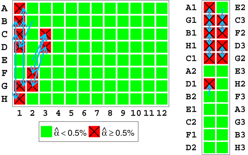
Abstract

Array genotyping is a cost-effective and widely used tool that enables assessment of up to millions of genetic markers in hundreds of thousands of individuals. Genotyping array data are typically highly accurate but sensitive to mixing of DNA samples from multiple individuals prior to or during genotyping. Contaminated samples can lead to genotyping errors and consequently cause false positive signals or reduce power of association analyses. Here, we propose a new method to identify contaminated samples and the sources of contamination within a genotyping batch. Through analysis of array intensity and genotype data from intentionally mixed samples and 22,366 samples of the Michigan Genomics Initiative, an ongoing biobank-based study, we show that our method can reliably estimate contamination. We also show that identifying sources of contamination can implicate problematic sample processing steps and guide process improvements. Compared to existing methods, our approach can estimate the proportion of contaminating DNA more accurately, eliminate the need for external databases of allele frequencies, and provide contamination estimates that are more robust to ancestral origin of the contaminating sample.

1. Introduction

Array genotyping is the standard method to genotype large numbers of individuals for genome-wide association studies (GWAS), consumer genomics, evaluation of copy number in clinical settings, and sample quality control prior to sequencing (Diskin et al., 2008). Consortium efforts now include millions of directly genotyped samples, and array genotyping has successfully been applied to traits as diverse as height (Marouli et al., 2017), body mass index (Locke et al., 2015), blood pressure (Hoffmann et al., 2017), type 2 diabetes (Mahajan et al., 2014), schizophrenia (Goes et al., 2015), and inflammatory bowel disease (Liu et al., 2015), among many others. When coupled with imputation, genotyping arrays can achieve a similar coverage of the genome to sequencing for a fraction of the cost (Y. Li, Willer, Ding, Scheet, & Abecasis, 2010).

Typically, genotyping arrays use fluorescent-tagged nucleotides or oligonucleotides that are specific to each allele of a genetic polymorphism. Measurements of allele-specific intensities are collected in parallel at 100,000s of loci, post-processed and clustered to distinguish genotypes at different bi-allelic markers (G. Li, 2016). These steps are sensitive to DNA sample contamination and mixing so that contaminated samples will have a higher probability of missing or erroneous calls that can result in a loss of power (Flickinger, Jun, Abecasis, Boehnke, & Kang, 2015) or in erroneous downstream inferences.

This DNA sample contamination is a common problem in large-scale studies. For example, the 1000 Genomes project reported that 3% of the sequenced samples were excluded due to high contamination (Flickinger et al., 2015). To address this problem, there are now several methods for detecting DNA contamination in both genotyping and sequencing data. Early methods flagged contaminated samples, but did not estimate the proportion of contamination (Homer et al., 2008). Newer methods like VerifyIDintensity and BAFRegress estimate contamination proportions by examining sample-specific shifts in allele intensity clusters for each genotype (Jun et al., 2012). Similar methods exist to examine the proportion of reads in sequencing data that are from contaminating DNA, for example ContEst and VerifyBAMID (Cibulskis et al., 2011; Jun et al., 2012). Contamination estimation has even been applied to array methylation data (Heiss & Just, 2018). Although our focus here is on within-species contamination, methods also exist for estimating cross-species contamination in sequencing data (Schmieder & Edwards, 2011). However, none of these methods can simultaneously estimate both contamination and its sources in genotyping array samples.

Here we present a new method, VICES (Verification of Intensity Contamination from Estimated Sources) that estimates contamination proportions and identifies contaminating samples in genotyping array data. VICES initially uses sample allele frequencies to estimate contamination and then revises this estimate by iteratively searching for sources of contamination among other genotyped samples. When the contaminating sample can be identified, our method provides improved estimates of contamination proportions compared to existing methods VerifyIDintensity and BAFRegress. Identifying contaminating samples also helps revise laboratory protocols to prevent future contamination. Finally, by examining data from ongoing studies, we show that VICES can help flag problematic sample processing steps where contamination occurred.

2. Methods

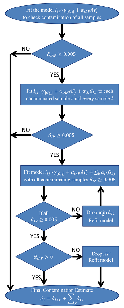
Our method has three steps: 1. identifying contaminated samples, 2. identifying likely contaminating samples for each contaminated sample, and 3. producing a final estimate of contamination, quantifying contributions from each contaminating sample (Figure 1).

Figure 1:

Flowchart of the contamination estimation algorithm. The flowchart shows how the algorithm progresses as contaminated samples are identified using allele frequencies, then potential contaminating samples are found for them and model selection performed to prune contaminating samples and calculate the final estimates.

We will first introduce some notation. We consider a set of individuals, each genotyped using an array. For each marker j, we assume two alleles, arbitrarily labelled A and B. We denote the frequency of B at this marker as AF_j. We let G_ij denote the estimated genotype for individual i at marker j, encoded as 0 (homozygous for A), 1 (homozygous for B), or ½ (heterozygous). Following convention, we let I_ij denote the relative intensity of the B-allele probe, measured on a 0 to 1 scale by interpolating allele intensity values with respect to the centers of the three genotype clusters and truncating any values that fall outside the 0 to 1 range (Illumina, 2010). Although other definitions of I_ij are possible, we choose this one because estimates are readily available from Illumina genotyping software.

The following model relates I_ij of the sample being tested to its estimated genotype and to the genotypes of each potential contaminating sample. Let α_i be the total proportion of contaminating DNA in sample i and α_ik the proportion of DNA mixture from sample k.

$$E\left(I_{ij}\right)=\left(1-{\alpha }_i\right)G_{ij}+{\text{Σ}}_k{\alpha }_{ik}{G}_{kj}$$ (Equation 1)

Directly fitting this model performs poorly because even in the absence of contamination, average intensity I_ij ≤ 1 when G_ij = 1 and average intensity I_ij ≥ 0 when G_ij = 0. Instead, we fit three genotype specific background intensity values ${\gamma }_0$, ${\gamma }_{\raisebox{1ex}{$1$}\!\left/ \!\raisebox{-1ex}{$2$}\right.}$, and ${\gamma }_1$ which model the expected intensity for each genotype class. This results in the model:

$$E\left(I_{ij}\right)=\left(1-{\alpha }_i\right){\gamma }_{\left[G_{ij}\right]}+{\text{Σ}}_k{\alpha }_{ik}{\gamma }_{\left[G_{kj}\right]}$$ (Equation 2)

which requires numerical optimization to estimate the total contamination proportion, α_i, and the contamination proportions α_ik from each contaminating sample. Fitting the following linear regression model

$$E\left(I_{ij}\right)={\gamma }_{\left[G_{ij}\right]}+{\text{Σ}}_k{\alpha }_{ik}{G}_{kj}$$ (Equation 3)

Gave estimates within 0.1% of Equation 2 for the contamination proportion from each contaminating sample, α_ik, while using only a fraction of the computational time. The ${\gamma }_{\left[G_{ij}\right]}$ intercept terms allow for a different mean I_ij for each cluster of sample genotypes, with each α_ik coefficient having the convenient interpretation as the contamination proportion from sample k.

Identification of the contaminated and contaminating samples in a genotyping cohort, and estimation of the contamination proportion from each contaminating sample α_ik proceeds as follows:

2.1. Identification of contaminated samples

We substitute the contaminating sample genotypes in Equation 3 with the allele frequencies AF_j to obtain initial estimates of the contamination proportion α_i for each sample being considered. This enables us to exclude uncontaminated samples from the computationally intensive search for samples that contributed contaminating DNA.

We fit the following model to obtain ${\widehat{\alpha }}_{iAF}$, an initial estimate of the contamination proportion α_i:

$$E\left(I_{ij}\right)={\gamma }_{\left[G_{ij}\right]}+{\alpha }_{iAF}A{F}_j$$ (Equation 4)

When fitting this model, we recommend excluding any sites with minor allele frequency less than 0.1 to reduce the influence of monomorphic and rare variants on the parameter estimation.

If this first estimate of the contamination proportion based on allele frequencies, ${\widehat{\alpha }}_{iAF}$, is below a user-specified threshold T (we recommend T no less than 0.005), then we assume the sample is uncontaminated and estimation stops here. If it is above that threshold, then our method attempts to identify the contaminating samples among the other genotyped samples.

2.2. Find the samples that contributed contaminating DNA

After identifying the contaminated samples using allele frequencies, the next step is to estimate a set of likely samples that contributed DNA to them. To do this, we fit the following linear regression model where we regress allelic intensity on the contaminated sample genotypes, allele frequency, and the genotypes of each candidate contaminating sample in turn:

$$E\left(I_{ij}\right)={\gamma }_{\left[G_{ij}\right]}+{\alpha }_{iAF}A{F}_j+{\alpha }_{ik}{G}_{kj}$$ (Equation 5)

This step identifies a series of candidate contaminating samples for each contaminated sample. We specifically focus on pairings of contaminated and contaminating samples where the estimate of ${\widehat{\alpha }}_{ik}$ is greater than our contamination threshold T. For these potential combinations of contaminated and contaminating samples, we proceed to the final step to calculate an improved contamination estimate.

2.3. Fit the final model with all contaminating samples to produce a final estimate

After identifying likely contaminating samples, this final step fits the following regression:

$$E\left(I_{ij}\right)={\gamma }_{\left[G_{ij}\right]}+{\alpha }_{iAF}A{F}_j+{\text{Σ}}_k{\alpha }_{ik}{G}_{kj}$$ (Equation 6)

with the intensities I_ij and estimated genotypes G_ij of the contaminated sample, the allele frequencies AF_j, and the genotypes G_kj of all the samples whose estimated contribution ${\widehat{\alpha }}_{ik}$ to the contamination proportion was greater than the contamination threshold T.

Since contamination only affects I_ij at sites where G_ij ≠ G_kj, such sites tend to be highly polymorphic. As a result, any individual k’, even if it did not contribute DNA to sample i, is likely to have many G_ij ≠ G_k’j at those sites with large I_ij − G_ij, and can appear to explain some of the contamination. Therefore, the set of potential contaminating samples identified in Step 2 may include false positives. When the contributions of these “false positive” contaminating samples are estimated jointly with those of the true contaminating samples, we expect their ${\widehat{\alpha }}_{ik}$ coefficients to drop near zero. Therefore, we expect the best estimates of contamination proportions will be obtained after estimation in step 3 (using Equation 6). If at this point, there are any ${\widehat{\alpha }}_{ik}<T$, we exclude the sample with the smallest ${\widehat{\alpha }}_{ik}$ and refit the regression, repeating this step until we have excluded all candidate contaminating samples whose contributions ${\widehat{\alpha }}_{ik}$ are below T.

After inclusion of all contaminating samples, the background contamination estimate should also drop to near or below 0. We define background contamination as α_iAF in equation 6. To be consistent with this interpretation, once all samples with contamination contribution ${\widehat{\alpha }}_{ik}$ less than T are removed, this background contamination term α_iAF is also dropped if it is estimated ≤ 0 since the proportion of contaminating DNA from any source cannot be negative.

The final model and resulting estimate of contamination can be one of the following three possibilities:

1. The estimated contamination contribution from allele frequencies, ${\widehat{\alpha }}_{iAF}$, drops to or below 0 and the model is refit with the estimated contaminating samples only. The estimate of the total contamination proportion is then the sum of the contamination contribution from each estimated source, as in Equation 3:

   $$E\left(I_{ij}\right)={\gamma }_{\left[G_{ij}\right]}+{\text{Σ}}_k{\alpha }_{ik}{G}_{kj}$$
2. No contaminating samples remain in the model, leaving only the contamination contribution from allele frequencies. This results in the model in Equation 4 and the same contamination proportion estimated in Step 1:

   $$E\left(I_{ij}\right)={\gamma }_{\left[G_{ij}\right]}+{\alpha }_{iAF}A{F}_j$$
3. Both estimated contaminating samples and allele frequencies remain in the model. Then the ${\widehat{\alpha }}_{iAF}$ coefficient can be interpreted as the proportion of contamination that came either from outside the genotyping cohort or from contaminating samples in the cohort but at proportions that were too small to be estimated reliably. The estimate of the total contamination proportion is then the sum of the contamination contribution from the estimated sources and the contamination contribution from allele frequencies. In this scenario, the final model is as in Equation 6:

   $$E\left(I_{ij}\right)={\gamma }_{\left[G_{ij}\right]}+{\alpha }_{iAF}A{F}_j+{\text{Σ}}_k{\alpha }_{ik}{G}_{kj}$$

2.4. Implementation

We have implemented VICES in a free software package written in C++ and available for download at http://genome.sph.umich.edu/wiki/VICES.

2.5. Experimental Data

We analyzed contamination in two sets of genotyping data. These different data sets allowed us to quantify the effect of contamination in the context of different arrays and experiments. It also allowed us to compare the performance of VICES with previous contamination methods VerifyIDintensity and BAFRegress under different scenarios (Jun et al., 2012).

2.5.1. Intentionally Contaminated HapMap Samples

To evaluate the effect of contamination on genotype calling and the performance of our method, we used intensity data and genotype calls generated by Jun et al. (2012) from 34 samples that were intentional mixtures of DNA from 4 HapMap cell lines (International HapMap et al., 2010). The samples were 100:0, 0.5:99.5, 1:99, 2:98, 3:97, 5:95, and 10:90 mixtures of mixed European ancestry (CEU) samples NA07055 and NA06990, and 0:100, 0.5:99.5, 1:99, 2:98, 5:95, and 10:90 mixtures of Yoruban (YRI) samples NA19200 and NA18504 (Table 1) and genotyped on the Illumina MetaboChip (Voight et al., 2012) at 196,725 markers. We obtained contaminating sample genotypes and allele frequency estimates for contamination estimation from the 1000 Genomes Phase 3 version 5 at sites that overlapped with the MetaboChip (Genomes Project et al., 2015). We estimated contamination in these 34 samples using: (1) VICES with contaminating sample genotypes (VICES-Geno), (2) VICES with allele frequencies (VICES-AF), (3) VerifyIDintensity (VID) and (4) BAFRegress (BAFR). Specifically, we compared root-mean-squared-error (RMSE), bias, and trend in absolute error as contamination increased for the four sets of contamination estimates.

Table 1:

Composition of 34 mixtures of HapMap cell lines from NA06990, NA07055, NA18504, and NA19200. The contamination percentages are in bold.

No. Samples	NA06990 (CEU)	NA07055 (CEU)	NA18504 (YRI)	NA19200 (YRI)
6	0%	100%	0%	0%
2	99.5%	0.5%	0%	0%
2	99%	1%	0%	0%
2	98%	2%	0%	0%
2	97%	3%	0%	0%
2	95%	5%	0%	0%
2	90%	10%	0%	0%
6	0%	0%	100%	0%
2	0%	0%	99.5%	0.5%
2	0%	0%	99%	1%
2	0%	0%	98%	2%
2	0%	0%	95%	5%
2	0%	0%	90%	10%

For the estimates calculated using VICES-Geno, the contaminating sample was already known in each case, so we estimated the contamination proportion by fitting the model in Equation 3. For all mixtures of HapMap YRI cell lines, we used the 1000 Genomes genotypes from sample NA19200 to estimate contamination. For the uncontaminated CEU samples from NA07055, we randomly chose an unrelated CEU sample from 1000 Genomes, NA12776, to provide the contaminating sample genotypes to fit in the model. For the CEU mixture samples, we used the metabochip genotypes of NA07055 as the contaminating sample. We only used NA19200 genotypes at sites with minor allele frequency above 10% in in 661 African ancestry samples of the 1000 Genomes Project (AFR). Similarly, we only used NA12776 or NA07055 genotypes at sites with minor allele frequency above 10% in 503 European ancestry samples of the 1000 Genomes Project (EUR).

For the estimates calculated using VICES-AF, we regressed the Metabochip intensities on their respective genotypes and allele frequencies as in Equation 4. We used 1000 Genomes EUR allele frequencies to estimate contamination in the CEU samples and 1000 Genomes AFR allele frequencies to estimate contamination in the YRI samples. As in the previous, we only used allele frequencies with MAF above 10%. We used the same sets of allele frequencies to estimate contamination with BAFRegress and VerifyIDintensity. We ran BAFRegress with default settings and VerifyIDintensity using the per-marker analysis option recommended by the authors of the software (Jun et al., 2012).

We also used the intentionally mixed HapMap samples to illustrate the effect of using allele frequencies from a mis-specified population on contamination estimation with VICES-AF, BAFRegress, and VerifyIDintensity. For this analysis, we used the 1000 Genomes EUR allele frequencies to estimate contamination in the YRI samples, and the 1000 Genomes AFR allele frequencies to estimate contamination in the CEU samples. Again, we only used allele frequencies with MAF above 10% and the per-marker analysis option for VerifyIDintensity.

2.5.2. Michigan Genomics Initiative

Next, we compared estimates from VICES with VerifyIDintensity and BAFRegress, in a large genotyping study where contamination may have occurred unintentionally. For this, we used data from the Michigan Genomics Initiative (Fritsche et al., 2018), an ongoing study of genetic data and health records from patient volunteers at the University of Michigan Hospital. We used 22,366 samples genotyped at 603,583 markers on a customized Illumina Infinium HumanCoreExome-24 v1.0 array (Illumina, 2017). DNAs, extracted from blood, were assayed in batches of 288 to 576 samples (3–6 plates of 96 samples each) per run according to the Illumina Infinium HTS Assay Protocol Guide (Illumina, 2013). The smallest assay runs with 288 samples were combined with larger batches for genotype calling in GenomeStudio (Illumina, 2016), so sets of genotype calls ranged in size from 384 to 864 samples. We considered contamination between samples from different set of genotype calls to be unlikely, so we ran our method on each set of genotype calls separately using VICES with the default settings. We also ran VerifyIDintensity on each set of genotype calls separately and with the per-marker analysis option. BAFRegress was run under default settings. For both VerifyIDintensity and BAFRegress, we used variants that overlapped with the HumanCoreExome array and whose 1000 Genomes EUR MAF was above 10% at overlapping sites. VICES calculates allele frequencies for initial estimation so no external allele frequencies were used. The true contamination proportions were not known in MGI, but we were able to compare the concordance of the three methods’ contamination estimates, the proportion of samples with estimated contamination greater than 0.5%, and how strongly contamination estimates were correlated with the number of missing and excess heterozygous genotype calls as calculated by Plink 1.9 (Chang et al., 2015).

3. Results

3.1. HapMap

3.1.1. Shift in Probe Intensities - HapMap

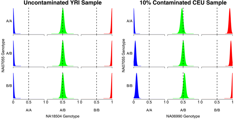
We examined how contamination changed overall intensity for homozygous A/A, heterozygous, and homozygous B/B genotypes. We saw that, in each case, intensity clusters were shifted towards the contaminant genotype. This result supports the validity of the assumption in Equation 2 that the intensities shift in proportion to the contamination and the genotypes of the contaminant sample. The kernel density plots in Figure 2 show the distributions of the intensities for an uncontaminated sample and for a sample contaminated at the 10% level, as a function of genotypes for the contaminating sample. The distribution of the intensities in the contaminated sample is shifted towards the genotypes of the contaminating sample (for example, when the contaminating sample has genotype B/B, all intensities are shifted towards the B allele). As expected, the distribution of intensities for the uncontaminated sample is independent of the genotypes of the potential contaminating sample.

Figure 2:

Kernel density plots showing the distribution of array probe intensities for an uncontaminated HapMap Yoruban sample (NA18504, left) and a 10% contaminated HapMap European sample (NA06990, right) as a function of the genotypes of NA07055. It is apparent that the intensities of the contaminated sample shift in the direction of NA07055 genotypes.

3.1.2. Estimation - HapMap

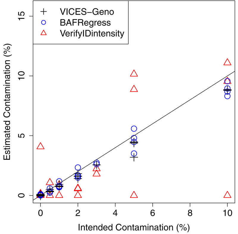
We next examined whether we could accurately estimate contamination in the intentionally mixed HapMap samples. These samples were prepared by Jun et al. (2012) to assess the performance of their own methods to estimate contamination. A total of 179,935 markers overlapped between the Metabochip and 1000 Genomes. Of these, we used AFR allele frequencies of 90,401 markers with MAF above 10% and EUR allele frequencies of 88,747 markers with MAF in EUR above 10%. Compared to the intended contamination, VICES-Geno had a root-mean-squared-error (RMSE) of 0.0057 and bias of −0.0035 across the 34 samples (Table 2, Figure 3). As contamination increased, the absolute error of VICES-Geno estimates increased on average by 0.0012 for each percentage increase in contamination. VICES-Geno performed better than VICES-AF, which had RMSE of 0.0068, bias of −0.0041, and an increase in absolute error of 0.0015 for each percentage increase in contamination. This shows an additional benefit in estimating contamination by using the genotypes of the contaminating sample as opposed to sample or population allele frequencies.

Table 2.

Root-mean-squared-error (RMSE), bias, and change in absolute error per 1% higher contamination of the three methods against the intended contamination of the 34 HapMap CEU samples.

	VICES-Geno	VICES-AF	BAFRegress	VerifyIDintensity
RMSE	0.0057	0.0068	0.0054	0.031
Bias	−0.0035	−0.0041	−0.0024	−0.0085
Increase in abs. error per 1% increase in contamination	0.0012	0.0015	0.0011	0.0056

Figure 3:

Comparison of estimates from our method using contaminating sample genotypes, BAFRegress, and VerifyIDintensity on the 34 mixtures of HapMap DNA to the intended contamination proportion.

VICES-Geno’s performance was within 0.001 of existing method BAFRegress on the three criteria and outperformed VerifyIDintensity by a much wider margin. BAFRegress had a RMSE of 0.0054, bias of −0.0024, and absolute error increased by 0.0011 for each percentage increase in contamination, while VerifyIDintensity had RMSE of 0.0310, bias of −0.0085, and absolute error increased by 0.0056 for each percentage increase in contamination (Figure 3). The results of this comparison are also summarized in Table 2.

3.1.3. Estimation with Misspecified Allele Frequencies - HapMap

We next evaluated the impact of ancestral population for reference allele frequencies on estimates of contamination. We expected this choice would have only a very limited impact for VICES-Geno as long as contaminating sample genotypes were available. However, the impact would be potentially larger for BAFRegress and VerifyIDintensity since they rely on estimated allele frequencies to estimate contamination.

We used 1000 Genomes allele frequencies calculated in EUR with MAF > 10% at 88,747 markers that overlapped with the Metabochip to estimate contamination in the intentionally mixed HapMap YRI samples. Similarly, we used 1000 Genomes allele frequencies calculated in AFR with MAF > 10% at 90,401 markers that overlapped with the Metabochip to estimate contamination in the CEU samples. Compared to the intended contamination, VICES-AF using mis-specified allele frequencies had RMSE of 0.0231, bias of −0.0140, and absolute error increased by 0.0057 for each percentage increase in contamination across the 34 samples. When the correct allele frequencies were used, VICES-AF had RMSE of 0.0068, bias of −0.0041, and a 0.0015 increase in absolute error for each percentage increase in contamination.

The other two methods also showed a similar drop in performance when using the misspecified allele frequencies. BAFRegress had a RMSE of 0.0261, bias of −0.0150, and the absolute error increased by 0.0065 for each percentage increase in contamination, while VerifyIDintensity had RMSE of 0.0312, bias of −0.0086, and the absolute error increased by 0.0056 for each percentage increase in contamination. The results of this comparison between our method, BAFRegress, and VerifyIDintensity with misspecified allele frequencies are also summarized in Table 3.

Table 3.

Root-mean-squared-error, bias, and change in absolute error per 1% higher contamination of the three methods against the intended contamination of the 34 intentionally mixed HapMap samples when 1000 Genomes allele frequencies from the incorrect population were used.

	VICES-AF	BAFRegress	VerifyIDintensity
RMSE	0.023	0.026	0.031
Bias	−0.014	−0.015	−0.0086
Increase in abs. error per 1% increase in contamination	0.0057	0.0065	0.0056

All three methods performed worse when the population for the allele frequencies was misspecified than when they were correctly specified, as shown in Table 2. This result implies that when using BAFRegress or VerifyIDintensity, prior knowledge of the ancestry of contaminating DNA is necessary to find contaminated samples and exclude their genotype calls from downstream analyses, an impractical step in a large GWAS cohort of diverse ancestry. This result highlights the benefit to estimating samples that contributed contaminating DNA so that estimation is not as sensitive to the choice of population for allele frequencies.

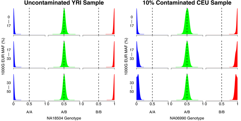
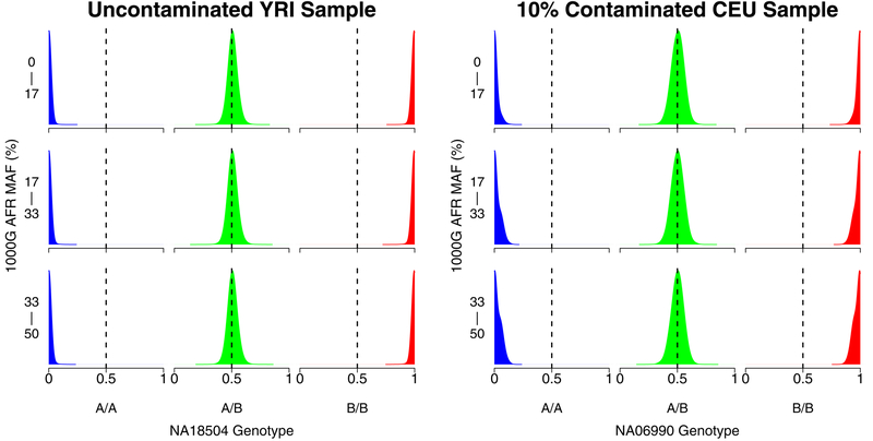
3.1.4. Shift in Allele Frequencies with Misspecified Allele Frequencies - HapMap

We further explored the previous point about how using misspecified allele frequencies can lead to an underestimation of contamination levels. Figure 4 shows the distribution of intensities for each genotype for a contaminated and an uncontaminated sample in different 1000 Genomes EUR minor allele frequency bins instead of contaminating sample genotypes as in Figure 2. As expected, contamination results in a greater shift in the intensity distribution at markers with higher allele frequencies. Figure 5 recapitulates Figure 4 but uses minor allele frequencies calculated from 1000 Genomes AFR individuals. As shown, the distribution of probe intensities is similar in the uncontaminated sample regardless of MAF of the population in which the MAFs were calculated. However, the shift in the intensity distribution at higher allele frequencies is less pronounced when using 1000 Genomes AFR MAFs compared to using 1000 Genomes EUR MAFs. This result highlights the benefit of using estimated contaminating sample genotypes for improving contamination estimation in genotyping samples.

Figure 4:

Kernel density plots showing the distribution of array probe intensities for an uncontaminated HapMap Yoruban sample (NA18504, left) and a 10% contaminated HapMap European sample (NA06990, right) at different 1000 Genomes European minor allele frequency (MAF) bins. The sample NA07055 that contributed DNA to the contaminated sample on the right is from the same ancestral population that the MAFs were calculated in, so using the MAFs to estimate contamination with a method like BAFRegress in this case would result in a good estimate for the intended contamination of 10%.

Figure 5:

Kernel density plots showing the distribution of array probe intensities for an uncontaminated HapMap Yoruban sample (NA18504, left) and a 10% contaminated HapMap European sample (NA06990, right) at different 1000 Genomes African minor allele frequency (MAF) bins. The sample NA07055 that contributed DNA to the contaminated sample on the right is European while the MAFs were calculated from African samples, so using the MAFs to estimate contamination with a method like BAFRegress in this case would result in a dramatic underestimate for the intended contamination of 10%.

3.2. Michigan Genomics Initiative (MGI)

3.2.1. Estimation - MGI

Our next aim was to investigate whether our method could accurately estimate contamination in a large-scale genotyping experiment. A test of the three methods in the 22,366 MGI samples suggests that VICES strikes a balance between the low estimates provided by BAFRegress and the higher estimates provided by VerifyIDintensity, consistent with our analysis of intentionally contaminated HapMap samples (see Figure 3, Table 2). Among the 22,366 samples, VICES found 354 with contamination greater than 0.5%, BAFRegress found 291 samples, while VerifyIDintensity found 4,498, or 20% of the samples tested.

This last result raised the question of why VerifyIDintensity estimated contamination greater than 0.5% for 4,188 samples for which both BAFRegress and VICES estimated contamination less than 0.5%. Upon investigation, it turned out that in samples where VICES estimated contamination less than 0.5%, the VerifyIDintensity estimates tended to be higher when there was a greater mean squared difference between the probe intensity and called genotype centroid (Figure 7). The same relationship was not seen in the BAFRegress or VICES estimates in the same set of samples. This result shows that VerifyIDintensity is prone to overestimating contamination in samples with greater variability in their probe intensities.

Figure 7:

Estimated contamination of the three methods as a function of mean-squared-error between intensity and called genotype, in 22,012 Michigan Genomics Initiative samples with contamination < 0.5% as estimated by VICES.

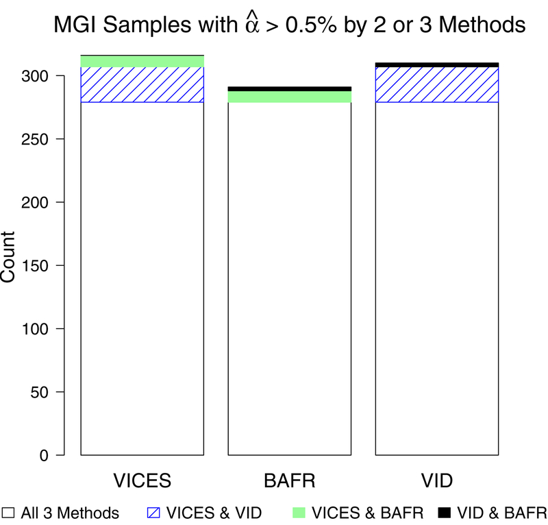
The true contamination proportions were not known in MGI, but we compared the estimates from the three methods to one another to determine which represented the best consensus. We found that the samples which VICES estimated as contaminated greater than 0.5% were validated more often by the other methods than the samples estimated as contaminated greater than 0.5% by BAFRegress or VerifyIDintensity. The bar plot in Figure 8 shows the counts for the number of samples with estimated contamination greater than 0.5% by at least two of the three methods, which also shows that VICES had the highest number of samples (316) with estimated contamination greater than 0.5% verified by at least one other method. VICES also had lower root-mean-squared-difference with estimates from BAFRegress (0.0075) and VerifyIDintensity (0.0062) than they did with each other (0.0089).

Figure 8:

Bar plot of the count of Michigan Genomics Initiative samples with estimated contamination greater than 0.5% by VICES, BAFRegress, or VerifyIDintensity and at least one other method.

Comparing the contamination estimates to call rate and excess heterozygosity of the MGI samples provided an independent metric which further supports the accuracy of VICES. Figures 9 and 10 show that all three methods exhibited the same relationship that, as estimated contamination increased, genotype call rates decreased and excess heterozygosity increased. However, the underestimation of BAFRegress was more pronounced in samples with a high level of contamination. BAFRegress did not estimate contamination greater than 13% for any sample, even for 11 samples that VICES and VerifyIDintensity both estimated as having contamination proportions greater than 20%. For this reason, the trend between estimated contamination and excess heterozygosity, and estimated contamination and call rate was weaker with the BAFRegress estimates (R² 0.03 for both call rate and excess heterozygosity) than VICES (R² 0.18 for call rate, R² 0.19 for excess heterozygosity) or VerifyIDintensity (R² 0.11 for call rate, R² 0.12 for excess heterozygosity).

Figure 9:

Comparing estimated contamination in 22,366 Michigan Genomics Initiative samples and their call rates. Left: VICES. Center: BAFRegress. Right: VerifyIDintensity. In all three plots, the red triangles denote the samples that had a contaminating sample detected by our method.

Figure 10:

Comparing estimated contamination in 22,366 MGI samples and excess heterozygosity as calculated using Plink 1.9. Left: VICES. Center: BAFRegress. Right: VerifyIDintensity. In all three plots, the red triangles denote the samples that had a contaminating sample detected by our method.

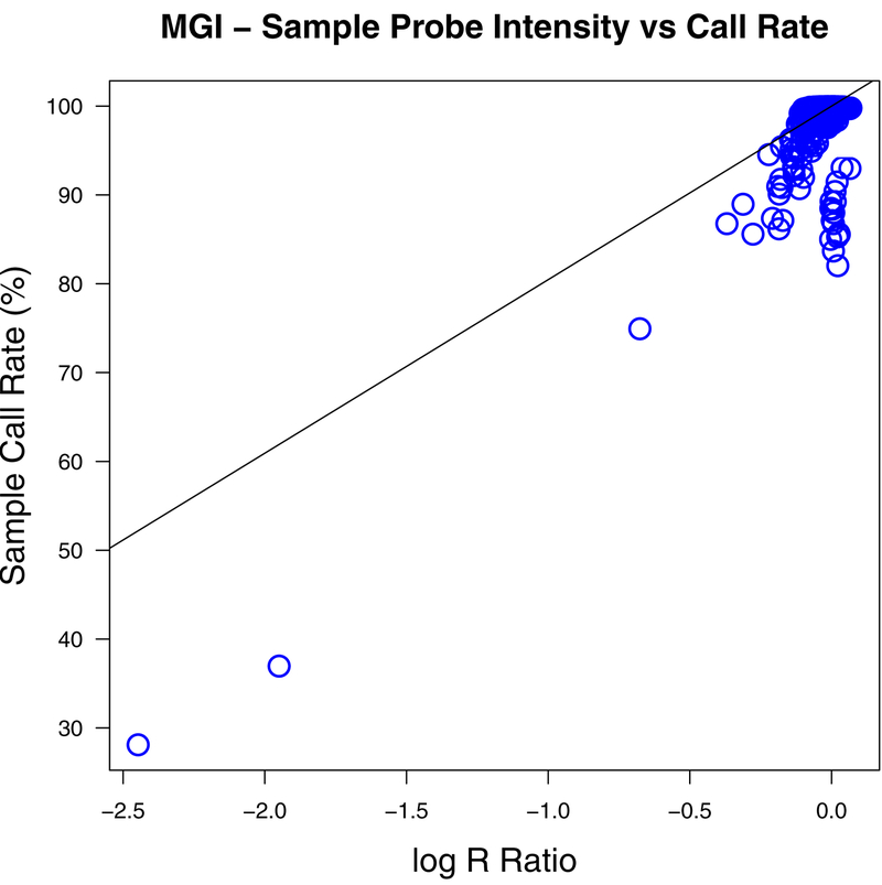
Since the plot of sample call rate against VICES estimated contamination in Figure 9 appeared to show two trend lines, we sought an explanation. Specifically, we observed that many contaminated samples had a lower call rate than would be predicted by their contamination as estimated by VICES (Figure 9, left panel). We found that log₂ R ratio, a measure of the average genotyping array probe intensity for a sample (Peiffer et al., 2006), was a strong predictor of call rate (R² 0.48, Figure 11). In Figure 12 we removed all 165 samples with log₂ R ratio 2 standard deviations below the mean before plotting sample call rate against estimated contamination. In this plot, compared to Figure 9, the relationship between contamination and call rate was stronger and more distinct (R² 0.71, 0.13, and 0.55 respectively for VICES, BAFRegress, and VerifyIDintensity). This result shows that this second trend line in Figure 9 was not due to underestimation by our method, but by heterogeneity in the array probe intensity among the samples.

Figure 11:

Scatterplot of sample call rate for 22,366 genotyped samples from the Michigan Genomics Initiative and average array probe intensity as measured by log₂ R ratio. The black line shows the regression fit to these data.

Figure 12:

Comparing estimated contamination against call rates in 22,201 Michigan Genomics Initiative samples that had average array probe intensity (defined as log₂ R ratio) greater than a cutoff set at 2 standard deviations below the mean. Left: VICES. Center: BAFRegress. Right: VerifyIDintensity. In all three plots, the red triangles denote the samples that had a contaminating sample detected by our method.

3.2.2. Contaminating Sample Search - MGI

We sought to evaluate how often our method could find contaminating samples and whether the estimates implicated a clear mechanism for contamination. We used the VICES results from the 22,366 samples genotyped in the Michigan Genomics Initiative (MGI) and found that our method found contaminating samples from the same set of genotype calls for 301 or 85% of the 354 samples with estimated contamination above 0.5%. A total of 365 contaminating samples were estimated. Of these, 342 or 94% were on the same sample processing plate of 96 samples as the contaminated sample, and 328 or 90% were on the same genotyping array of 24 samples, showing that VICES estimates of contaminating samples are not random, but in fact consistently implicate a step in the sample preparation and genotyping process where contamination often occurred.

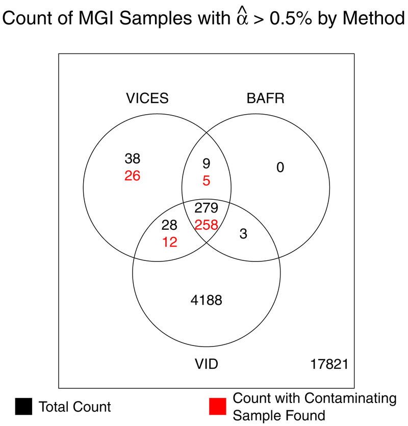
The number of contaminating samples offers further support for the accuracy of the VICES estimates relative to the other methods. Figure 6 shows that BAFRegress failed to detect contamination greater than 0.5% in 38 samples where VICES estimated such a level of contamination and found a contaminating sample, and VerifyIDintensity failed to detect contamination in 31 such samples. There were 26 such samples where neither BAFRegress nor VerifyIDintensity estimated contamination greater than 0.5%. These results suggest that BAFRegress and VerifyIDintensity may be prone to false negatives in contamination estimation, allowing contaminated samples through QC filters.

Figure 6:

Venn diagram showing (black) the count of all Michigan Genomics Initiative samples with estimated contamination greater than 0.5% by VICES, BAFRegress (BAFR), or VerifyIDintensity (VID) or any combination of the three methods, and (red) the count with estimated contamination greater than 0.5% and a contaminating sample found by VICES.

Based on the data in Figure 6, we wondered if any of the samples estimated as contaminated by VICES but not all three methods were false positives. One reason is that VICES found contaminating samples for a higher proportion (92%) of the 279 samples with estimated contamination greater than 0.5% by all three methods than in the 75 samples estimated as contaminated greater than 0.5% by VICES alone or by VICES and only one other method (57%). One explanation is that VICES estimated much lower contamination for the samples that were estimated to be uncontaminated by either BAFRegress or VerifyIDintensity. VICES estimated 48 (64%) of the 75 samples (estimated as contaminated by VICES but not all three methods) to be contaminated below 1%, compared to 28 (10%) of the 279 samples estimated as contaminated by all three methods. Small discrepancies in the estimates between the three methods may have pushed the estimates for some samples either just above or just below the contamination threshold T for a subset of the methods. For this reason, we expect that VICES will have more difficulty estimating sources of contamination for samples with borderline detectable contamination than for samples with high contamination.

In addition to improving estimation, finding the contaminating samples enables understanding and troubleshooting the cause of contamination. In the MGI samples, Figure 13 shows that the contaminated samples as estimated by VICES appear adjacent to one another on both the sample processing plate and the genotyping array. Running the contaminating sample search algorithm reveals that the estimated contaminating samples for each contaminated sample were adjacent to it on the array but not the processing plate. Since it would be more difficult to explain the pattern between contaminating and contaminated samples on the processing plate, this constitutes strong evidence for contamination occurring on the genotyping array between adjacent inlet ports during sample loading or array sections during hybridization due to leaky seals.

Figure 13:

Left: Eight contaminated samples as they appeared on part of the sample preparation plate. The letters to the left of the plate indicate the rows and numbers below indicate columns. Arrows indicate our method’s estimates for which sample contributed DNA to each contaminated sample. Right: The position of the same samples on the genotyping array. Letters and numbers indicate the row and column of the plate from which the samples were transferred. Arrows have the same interpretation.

This figure shows that the contaminated samples are adjacent to their contaminating sample on the array, while far apart and without a clear pattern on the processing plate. The relative ease of explaining the pattern of adjacent mixing on the array compared to the processing plate suggests that the DNA mixture occurred on the array itself.

4. Discussion

Contamination, or the mixture of DNA from multiple individuals prior to genotyping, decreases the quality of genotypes. Since genotyping arrays remain the predominant tool in genetic association studies, the ability to accurately diagnose contaminating DNA and its sources has the potential to improve data quality checks and data production for many genetic studies. Our results show that our method outperforms previous methods and can reliably find the contaminating samples, even at small contamination proportions. It can also perform contamination estimation in genotyping cohorts of mixed ancestry without relying on external allele frequency information or knowledge of the population origin of the contaminating samples. This feature makes the software appropriate for a wide range of genetic association studies. We also illustrate how one can conclude that contamination occurred on a genotyping array as opposed to during other steps in sample preparation, which may lead to improved genotyping protocols.

One of our central findings is that, compared to estimating contamination and its sources separately, doing so jointly, as described here, improves both and gives users of VICES a more useful combination of results. After contamination has been detected, researchers may be faced with several follow-up questions. For example, should a contaminated sample be excluded from downstream analyses? Can a sample be re-genotyped and yield uncontaminated genotype calls? Or is a sample’s DNA fit for whole-genome or whole-exome sequencing? VICES gives researchers accurate information to answer to these questions.

The above analysis illuminated several ways in which contamination and contaminating sample identification can be further improved. One remaining issue is that the deviations in array probe intensities caused by contamination can appear to be correlated to the genotypes of any individual, and not only the contaminating sample. We observed a similar effect at the population level, with the shift in allele frequencies showing the strongest correlation with frequencies in the contaminating sample population but weaker correlation when the contaminating population allele frequencies were misspecified.

This correlation between probe intensities and the genotypes of a sample that did not contribute DNA can be partially mitigated by including the sample allele frequencies in the regression as in Equations 5 and 6. However, at particularly high levels of contamination (greater than 25%) many false positive contaminating samples may still be identified. This problem can be improved by increasing the contaminating sample threshold for highly contaminated samples instead of the default threshold of 0.5%. There are alternatives to threshold based selection of contaminating samples that may be worthy of future exploration. For example, instead of including samples in the final model based on a point estimate for contamination contribution, inclusion could have been decided by p-value or false discovery rate-adjusted q-value, or estimating inflation in contamination contribution estimates.

An alternative strategy to make the contamination estimates more robust to the genetic ancestry of the contaminating DNA could be to iteratively estimate the ancestry of the contaminating allele frequencies instead of using the fixed allele frequencies of the sample or population. Such an approach could result in more accurate contamination estimates when no contaminating sample is found or could be used to narrow the search by the ancestry of the contaminating sample, resulting in greater computational efficiency. However, we have found that using contaminating sample genotypes improves contamination estimates compared to using population allele frequencies, even when the contaminating samples’ population is correctly specified (Table 2). Furthermore, using population allele frequencies, the user would not gain any insight as to how contamination occurred in their study.

In addition, several potential extensions or adaptations of this method exist. For example, a cross-array contamination check might be useful in studies where multiple arrays are used. In addition, the method could be adapted to impute missing and incorrect calls to salvage contaminated samples, as the CleanCall package does with contaminated sequencing data (Flickinger et al., 2015). Our own preliminary analyses suggest this would reduce the rate of missing and incorrect genotype calls in contaminated samples.

Genotype probe intensities are approximately normally distributed around the values of 0, ½, and 1 (depending on the underlying genotype), with truncation resulting in additional point masses at 0 and 1. Contaminating DNA results in a proportional shift in these distributions, as reflected in Figure 2. In principle, direct modeling of this intensity distribution (see Appendix) would enable us to predict the distribution of probe intensities for samples with different degrees of contamination, to model resulting increases in missing genotype rates (when intensities are drawn from the shifted distributions they will fall more often in ambiguous regions that lie between two expected genotype clusters) and in genotyping error rates. These models would allow predictions of the impact of genotyping error rate on power (as in Sobel, Papp, and Lange (2002)) or, potentially, methods for association analysis that model the underlying intensity data directly rather than relying on discrete genotype calls (as done in Kim, Gordon, Sebat, Ye, and Finch (2008) for structural variants, for example).

In our own work, we often must decide on acceptable thresholds for sample contamination. For simple regression-based approaches that model phenotypes as a function of genotypes and covariates, it’s tempting to be lenient and analyze samples that have modest amounts of contamination – after all, a contaminated sample with a few erroneous genotypes will still provide some useful information, albeit less information than an uncontaminated sample. However, many modern genetic analyses include additional analysis steps that involve sharing of information across samples – these steps might include haplotype estimation (which relies on identification of shared IBD segments between samples and is a key step in genotype imputation analyses) and also estimation of genetic kinship matrices or principal components of ancestry (which are also key steps for modern large scale genetic analyses that include related individuals or samples of diverse ancestry). In our experience, contaminated samples can have more deleterious effects for these analyses, corrupting the information contributed by other uncontaminated samples. Empirically, we typically recommend that samples with contamination greater than ~1% to 3% should be excluded from downstream analyses.

In conclusion, we have introduced VICES, a method that performs joint estimation of contamination and its sources in genotyping array samples. This innovation results in more accurate contamination estimates which are robust in genotyping cohorts of diverse ancestry. VICES allows researchers to estimate contamination easily without importing allele frequencies and provides additional information on how their samples were contaminated, so that it can be prevented or dealt with more effectively.

References

- Chang CC, Chow CC, Tellier LC, Vattikuti S, Purcell SM, & Lee JJ (2015). Second-generation PLINK: rising to the challenge of larger and richer datasets. GigaScience, 4, 8 eCollection 2015. doi: 10.1186/s13742-015-0047-8 [doi] [DOI] [PMC free article] [PubMed] [Google Scholar]
- Cibulskis K, McKenna A, Fennell T, Banks E, DePristo M, & Getz G (2011). ContEst: estimating cross-contamination of human samples in next-generation sequencing data. Bioinformatics (Oxford, England), 27(18), 2601–2602. doi: 10.1093/bioinformatics/btr446 [doi] [DOI] [PMC free article] [PubMed] [Google Scholar]
- Diskin SJ, Li M, Hou C, Yang S, Glessner J, Hakonarson H, … Wang K (2008). Adjustment of genomic waves in signal intensities from whole-genome SNP genotyping platforms. Nucleic acids research, 36(19), e126. doi: 10.1093/nar/gkn556 [doi] [DOI] [PMC free article] [PubMed] [Google Scholar]
- Flickinger M, Jun G, Abecasis GR, Boehnke M, & Kang HM (2015). Correcting for Sample Contamination in Genotype Calling of DNA Sequence Data. American Journal of Human Genetics, 97(2), 284–290. doi: 10.1016/j.ajhg.2015.07.002 [doi] [DOI] [PMC free article] [PubMed] [Google Scholar]
- Fritsche LG, Gruber SB, Wu Z, Schmidt EM, Zawistowski M, Moser SE, … Mukherjee B (2018). Association of Polygenic Risk Scores for Multiple Cancers in a Phenome-wide Study: Results from The Michigan Genomics Initiative. Am J Hum Genet, 102(6), 1048–1061. doi: 10.1016/j.ajhg.2018.04.001 [DOI] [PMC free article] [PubMed] [Google Scholar]
- Genomes Project C, Auton A, Brooks LD, Durbin RM, Garrison EP, Kang HM, … Abecasis GR (2015). A global reference for human genetic variation. Nature, 526(7571), 68–74. doi: 10.1038/nature15393 [DOI] [PMC free article] [PubMed] [Google Scholar]
- Goes FS, McGrath J, Avramopoulos D, Wolyniec P, Pirooznia M, Ruczinski I, … Pulver AE (2015). Genome-wide association study of schizophrenia in Ashkenazi Jews. American journal of medical genetics.Part B, Neuropsychiatric genetics : the official publication of the International Society of Psychiatric Genetics, 168(8), 649–659. doi: 10.1002/ajmg.b.32349 [doi] [DOI] [PubMed] [Google Scholar]
- Heiss JA, & Just AC (2018). Identifying mislabeled and contaminated DNA methylation microarray data: an extended quality control toolset with examples from GEO. Clin Epigenetics, 10, 73. doi: 10.1186/s13148-018-0504-1 [DOI] [PMC free article] [PubMed] [Google Scholar]
- Hoffmann TJ, Ehret GB, Nandakumar P, Ranatunga D, Schaefer C, Kwok PY, … Risch N (2017). Genome-wide association analyses using electronic health records identify new loci influencing blood pressure variation. Nature genetics, 49(1), 54–64. doi: 10.1038/ng.3715 [doi] [DOI] [PMC free article] [PubMed] [Google Scholar]
- Homer N, Szelinger S, Redman M, Duggan D, Tembe W, Muehling J, … Craig DW (2008). Resolving individuals contributing trace amounts of DNA to highly complex mixtures using high-density SNP genotyping microarrays. PLoS genetics, 4(8), e1000167. doi: 10.1371/journal.pgen.1000167 [doi] [DOI] [PMC free article] [PubMed] [Google Scholar]
- Illumina (2013). Infinium® HTS Assay Protocol Guide. San Diego, CA. [Google Scholar]
- Illumina (2016). GenomeStudio® Genotyping Module v2.0 Software Guide. San Diego, CA. [Google Scholar]
- Illumina. (2017). Infinium ® CoreExome-24 v1.2 BeadChip. [Google Scholar]
- International HapMap C, Altshuler DM, Gibbs RA, Peltonen L, Altshuler DM, Gibbs RA, … McEwen JE (2010). Integrating common and rare genetic variation in diverse human populations. Nature, 467(7311), 52–58. doi: 10.1038/nature09298 [DOI] [PMC free article] [PubMed] [Google Scholar]
- Jun G, Flickinger M, Hetrick KN, Romm JM, Doheny KF, Abecasis GR, … Kang HM (2012). Detecting and estimating contamination of human DNA samples in sequencing and array-based genotype data. American Journal of Human Genetics, 91(5), 839–848. doi: 10.1016/j.ajhg.2012.09.004 [doi] [DOI] [PMC free article] [PubMed] [Google Scholar]
- Kim W, Gordon D, Sebat J, Ye KQ, & Finch SJ (2008). Computing power and sample size for case-control association studies with copy number polymorphism: application of mixture-based likelihood ratio test. PloS one, 3(10), e3475. doi: 10.1371/journal.pone.0003475 [DOI] [PMC free article] [PubMed] [Google Scholar]
- Li G (2016). A new model calling procedure for Illumina BeadArray data. BMC genetics, 17(1), 90. doi: 10.1186/s12863-016-0398-x [DOI] [PMC free article] [PubMed] [Google Scholar]
- Li Y, Willer CJ, Ding J, Scheet P, & Abecasis GR (2010). MaCH: using sequence and genotype data to estimate haplotypes and unobserved genotypes. Genetic epidemiology, 34(8), 816–834. doi: 10.1002/gepi.20533 [doi] [DOI] [PMC free article] [PubMed] [Google Scholar]
- Liu JZ, van Sommeren S, Huang H, Ng SC, Alberts R, Takahashi A, … Weersma RK (2015). Association analyses identify 38 susceptibility loci for inflammatory bowel disease and highlight shared genetic risk across populations. Nature genetics, 47(9), 979–986. doi: 10.1038/ng.3359 [doi] [DOI] [PMC free article] [PubMed] [Google Scholar]
- Locke AE, Kahali B, Berndt SI, Justice AE, Pers TH, Day FR, … Speliotes EK (2015). Genetic studies of body mass index yield new insights for obesity biology. Nature, 518(7538), 197–206. doi: 10.1038/nature14177 [doi] [DOI] [PMC free article] [PubMed] [Google Scholar]
- Mahajan A, Go MJ, Zhang W, Below JE, Gaulton KJ, Ferreira T, … Morris AP (2014). Genome-wide trans-ancestry meta-analysis provides insight into the genetic architecture of type 2 diabetes susceptibility. Nature genetics, 46, 234. doi:10.1038/ng.289710.1038/ng.2897https://www.nature.com/articles/ng.2897#supplementary-informationhttps://www.nature.com/articles/ng.2897#supplementary-information [DOI] [PMC free article] [PubMed] [Google Scholar]
- Marouli E, Graff M, Medina-Gomez C, Lo KS, Wood AR, Kjaer TR, … Lettre G (2017). Rare and low-frequency coding variants alter human adult height. Nature, 542(7640), 186–190. doi: 10.1038/nature21039 [doi] [DOI] [PMC free article] [PubMed] [Google Scholar]
- Peiffer DA, Le JM, Steemers FJ, Chang W, Jenniges T, Garcia F, … Gunderson KL (2006). High-resolution genomic profiling of chromosomal aberrations using Infinium whole-genome genotyping. Genome Res, 16(9), 1136–1148. doi: 10.1101/gr.5402306 [DOI] [PMC free article] [PubMed] [Google Scholar]
- Schmieder R, & Edwards R (2011). Fast identification and removal of sequence contamination from genomic and metagenomic datasets. PloS one, 6(3), e17288. doi: 10.1371/journal.pone.0017288 [doi] [DOI] [PMC free article] [PubMed] [Google Scholar]
- Sobel E, Papp JC, & Lange K (2002). Detection and integration of genotyping errors in statistical genetics. Am J Hum Genet, 70(2), 496–508. doi: 10.1086/338920 [DOI] [PMC free article] [PubMed] [Google Scholar]
- Voight BF, Kang HM, Ding J, Palmer CD, Sidore C, Chines PS, … Boehnke M (2012). The metabochip, a custom genotyping array for genetic studies of metabolic, cardiovascular, and anthropometric traits. PLoS Genet, 8(8), e1002793. doi: 10.1371/journal.pgen.1002793 [DOI] [PMC free article] [PubMed] [Google Scholar]
Associated Data
This section collects any data citations, data availability statements, or supplementary materials included in this article.