

Abstract
Automated cell segmentation and tracking enables the quantification of static and dynamic cell characteristics and is significant for disease diagnosis, treatment, drug development and other biomedical applications. This paper introduces a method for fully automated cell tracking, lineage construction, and quantification. Cell detection is performed in the joint spatio-temporal domain by a motion diffusion-based Partial Differential Equation (PDE) combined with energy minimizing active contours. In the tracking stage, we adopt a variational joint local-global optical flow technique to determine the motion vector field. We utilize the predicted cell motion jointly with spatial cell features to define a maximum likelihood criterion to find inter-frame cell correspondences assuming Markov dependency. We formulate cell tracking and cell event detection as a graph partitioning problem. We propose a solution obtained by minimization of a global cost function defined over the set of all cell tracks. We construct a cell lineage tree that represents the cell tracks and cell events. Finally, we compute morphological, motility, and diffusivity measures and validate cell tracking against manually generated reference standards. The automated tracking method applied to reference segmentation maps produces an average tracking accuracy score (TRA) of 99%, and the fully automated segmentation and tracking system produces average TRA of 89%.
Keywords: Cell tracking, cell event detection and handling, graph algorithms, motion analysis
1. Introduction
Studies of living organisms in biology and medicine require the analysis of their static and dynamic properties. Advances in imaging technologies have enabled the acquisition of time-lapse sequences of 2D and 3D data at the cellular and molecular level. Research in medicine and biology has become increasingly dependent on quantitative analysis of this type of imaging data [1] for extracting information about cell metabolism, growth, reaction to stimuli, and reproduction [2]. The process of identification and tracking of each cell in an imaging sequence is necessary for measuring static and dynamic cell attributes.
Quantitative analysis includes the study of cell morphometry, such as the cells’ shape and their dynamic characteristics in a sequence including the cell lifetime, motility, number of divisions, and morphological changes with time among other characteristics. The quantitative analysis of time-lapse microscopy images is a key for detection of disease patterns and can be used in decision making to make a reliable diagnosis. Research in pathology is a very significant step for diagnosis of a large number of diseases including most cancers. The ability to non-invasively track the delivery of various therapeutic cells (e.g. T-cells and stem cells) to the tumor site, and subsequent proliferation of these cells, would allow better understanding of the mechanisms of cancer development and intervention. Moreover, data collected from individual patients at the anatomical, cellular and molecular levels, offer unprecedented possibilities to design personalized therapies. Studies of disease mechanisms are valuable for clinical research areas such as stem cell research, tissue engineering, drug discovery, genomics, and proteomics. Morphological changes correlate with disease progression. Study of cell lineage relationships is significant for stem cell research, and disease etiology and progression studies [3], [4]. The statistical analysis of the tracking measurements will assist researchers to more precisely track the genetics of individual cells and detect and understand cell behavior and abnormalities. These applications depend on accurate cell tracking of individual cells that display various behaviors including mitosis, merging, rapid movement, and entering and leaving the field of view.
The data size of a single cell image sequence is typically in the range of hundreds of megabytes. Diagnosing a disease after manually analyzing numerous data requires intensive and laborious work and long time. Furthermore, manual analysis is dependent on the level of experience of the human operator, and is almost certainly non-reproducible. As a consequence, the use of automatic analysis and quantification can significantly improve the reproducibility, efficiency, and accuracy of cell studies, and overall benefit the patient.
Cell tracking methodologies can be divided into (i) tracking by model evolution and (ii) tracking by detection.
Model Evolution Methods –
These techniques integrate the stages of segmentation and tracking into a joint model that represents the cell regions and their evolution with time. In this framework topological changes may account for cell events. Model Evolution methods frequently utilize parametric or implicit active contour models. Active contour methods for image segmentation allow a contour to deform to partition an image into regions. Deformable models try to fit one frame and use the result as initialization in the evolution model of the next frame. The association step is implicitly solved and established. However these techniques may require topology constraints and are computationally demanding especially for sequences of high cell density.
Parametric active contour models use explicit representations of the cell contours and perform segmentation by energy functional minimization [5], [6]. The classic snake methods cannot address topological changes related to cell events therefore they required some adjustments.
Implicit active contour models are often implemented with level sets [7], [8], [9]. The primary drawback, however, is that they are slow to compute. The level set can be initialized manually as an initial contour, or automatically by leveraging prior information about the shape and other characteristics of cells to track multiple cells [10]. Zhang et al [11] proposed coupled geometric active contours and used one level set function for each cell. The coupling constraints are applied to avoid cell overlapping. Dufour et al [12] extended this framework to 3D analysis.
Tracking by Detection –
These approaches typically detect the cells in each frame and then match cells between consecutive frames. The cell detection stage is achieved by image segmentation. The cell matching stage is completed by data association and cell correspondence techniques. Their main advantages of tracking by detection techniques are that they (i) can work on lower imaging frequencies than the model evolution techniques, (ii) involve advanced data association techniques for tracking, and (iii) separate the segmentation and tracking tasks, therefore different segmentation techniques can be used with a single tracking algorithm. Cell detection may be achieved by image segmentation techniques based on intensity, texture or gradient information [13], [14], [15], [16]. Feature-based segmentation techniques have been utilized for cell detection as described in [16], [17], [18]. Several deep learning approaches have also been proposed for cell detection, segmentation and classification in digital pathology and microscopy applications and have produced promising results [19], [20], [21]. However, most of the deep learning-based models do not implement a complete cell tracking system that requires cell matching and cell event handling stages.
Cell matching techniques often times use probabilistic functions between frames. Data association techniques that perform cell linking may be categorized into Bayesian and Non-Bayesian. Bayesian approaches compute the full distribution in Data Association space based on prior and posterior information. Non-Bayesian approaches find the Nearest Neighbor as the maximum likelihood estimate from all the Data Association possible solutions. Tracking by detection techniques may face challenges in mitosis tracking and when touching cells are segmented as a single cell. In previous reports in the literature, the authors in [22] used seeded watershed to address touching cells, followed by feature-based cell matching. They performed image-by-image track linking by means of integer programming. Yang et al [23] proposed to use watershed and mean shift to identify cell cycle progression but did not construct cell lineage.
In the tracking stage, when we encounter increasing cell density, the temporal association step requires sophisticated strategies to deal with one-to-many and many-to-one matching problems [8], [13], [14], [24]. In [13] image-by-image linking is accomplished using integer programming. Padfield et al [8] introduced a coupled minimum-cost flow algorithm for mitosis and merging events coupled with some operations on particular edges. They used linear programming to choose the edges of graphically represented constraints. In contrast to image-by-image linking techniques, batch algorithms use information from future frames or the complete image sequence to create cell tracks and detect cell events [25], [26]. The authors in [27] proposed a batch algorithm that optimizes a probabilistic scoring function and may address false positives and false negatives in detection stage. It can also handle cell mitosis, apoptosis and other cell events.
Another subgroup of methods combines detection and data association using probabilistic prediction models. These methods predict global motion and characteristic parameters of the objects. Earlier approaches used Kalman filtering followed by Particle Filtering techniques [15], [28]. They use sets of random samples to describe the most likely states of a system. They use the temporal structure of distributions and determine the measurements using importance sampling. Particle filters work well for a small and fixed number of cells. In the approach proposed in [29], the authors used marker controlled watershed and region merging with context information for cell detection and delineation. They performed tracking using modified mean shift and Kalman filtering.
The aim of this work is to develop automated methods that successfully detect and track cells enabling the analysis of their static and dynamic behavior including cell morphology, cell migration, and changes in cell states (mitosis and apoptosis, for example). To reach these objectives we introduce automated techniques for cell detection, segmentation, tracking, construction of lineage trees of progenitor cells, and cell quantification. Overall one may argue that many approaches to cell tracking have been developed in the past, but most are focused on the same type of optical imaging techniques, require extensive post-processing, and are parameter intensive.
The tasks of automatic cell detection, segmentation, and tracking in time-lapse fluorescent microscopy images pose a difficult problem due to high variability in images because of numerous factors like differences in slide preparation (fluorescent concentration, presence of foreign artifacts, time to prepare the sample, and time between each time lapse image for the same sample, etc) and image acquisition (corruption by different types of noise, specific features of the microscope such as resolution and contrast limitations, etc). To be able to capture fluorescent microscopy images and observe live cell processes, like cell migration, apoptosis and proliferation, light exposure is kept minimal to reduce the photodamage, but this reduces the image quality [30], [31], [32].
We propose a fully automated tracking method to overcome these challenges and achieve high level of accuracy in these different cases. We outline the key contributions of this work next. (i) In the cell matching stage, we utilize the predicted cell motion in a probabilistic Maximum Likelihood Bayesian decision framework assuming Markov dependency to find cell correspondences between consecutive frames. (ii) In cell event detection, we find a solution that minimizes a global cost function, given cell neighborhood constraints, defined over the set of all cell tracks to perform track linking and to identify the cell states in the time-lapse sequence. Our system automatically constructs the lineages of proliferating migrating cells, which is a critical and required step for understanding cell behaviors. It produces measurements of static and dynamic cell attributes. The proposed system is applicable to varying cell shapes, types, and densities and image sequences of reduced image quality. Overall, it enables accurate quantitative analysis of cell events, and provides a valuable tool for high-throughput biological studies.
In section 2, we present our proposed cell tracking method where we describe the pre-tracking stage, followed by an overview of the motion estimation and optical flow methods. We also introduce the combined local-global optical flow technique that we applied to our data, our likelihood-based bi-frame cell matching technique to link cells between frames, the proposed algorithms to create cell tracks and the acyclic graph, and cell event handling. In section 3, we show our cell tracking experiments and validation results and in section 4 we summarize the main findings of this work.
2. Method Overview
The goal of cell tracking is to identify all cells throughout the time-lapse sequence in order to follow their motion and detect the main events such as migration, mitosis, apoptosis, entering and leaving the field of view. Our method belongs to the category of tracking by detection. It uses cell indicator functions of each frame produced by our cell delineation technique to perform cell tracking and quantification. We propose a method for automated tracking of biological cells in time-lapse microscopy by motion prediction and minimization of a global probabilistic function for each set of cell tracks. We identify cell events by backtracking the cell track stack and forming new tracks to determine a partition of the complete track set.
As seen in Fig. 1, we first apply cell detection and delineation [33]. A pre-tracking stage is required to separate cell clusters to reduce under-segmentation, and to compute cell characteristics to be used for probabilistic cell matching and cell quantification. Then we estimate the cell motion by use of a variational multi-scale optical flow technique. Next, we apply the motion field to calculate warped cells and we apply a maximum likelihood decision approach on a probabilistic function to find cell correspondences. We then construct the cell linked lists to represent cell tracks and we backtrace the lists to detect overlapping tracks and identify and handle the cell events. After finding all cell events we construct the cell lineage tree that stores and visualizes the cell events. In addition, we calculate cell characteristics and their evolution with time to perform quantitative analysis and visualization.
Fig. 1.
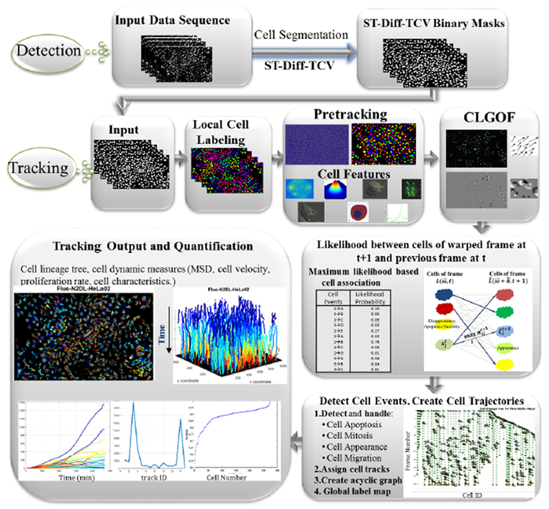
The main stages of the proposed cell tracking system.
We pursue a solution of the cell detection problem in the joint spatio-temporal domain to overcome weaknesses of previous works that operate only on the spatial domain. We employ a PDE-based formulation of spatio-temporal motion diffusion to detect the cell motion [34], [35]. We apply an intensity standardization technique to address intensity variability complicating frame-to-frame analysis in differential techniques. To refine cell delineation accuracy produced by motion diffusion-based segmentation, we use energy minimizing geometric active contours that assume a piece-wise constant image region model as a special case of the Mumford-Shah segmentation framework. Furthermore, we perform temporal linking of the region-based level sets to allow for faster convergence and to resolve non-convexity that affects energy-based minimization that is typical in image analysis inverse problems [33].
A tracking algorithm ideally should have the capability to address the main cell events that occur in a sequence. These events are (i) Cell Mitosis: division of a cell into two daughters (ii) Cell Disappearance: cell leaving field of view or collision (iii) Cell Apoptosis/Necrosis: death of a cell (iv) New Entering Cell: cell entering the field of view, and (v) Cell Reappearance: cell re-entering the field of view.
The association problem is usually the most complex and most challenging stage of the tracking system. By increasing the number of cells, the complexity of the linking problem increases exponentially. Changes in cell shape such as cell stretching may also cause false appearances due to cell detection discontinuities. Fig. 2a depicts a model of the cell events of migration, mitosis, disappearance and appearance. Fig. 2b displays a pair of consecutive frames selected from an image sequence dataset that we use for our experiments. Furthermore, Fig. 2b contains all the detectable cell events that may occur. Cell event detection usually follows cell tracking and requires analysis of cell tracks.
Fig. 2.
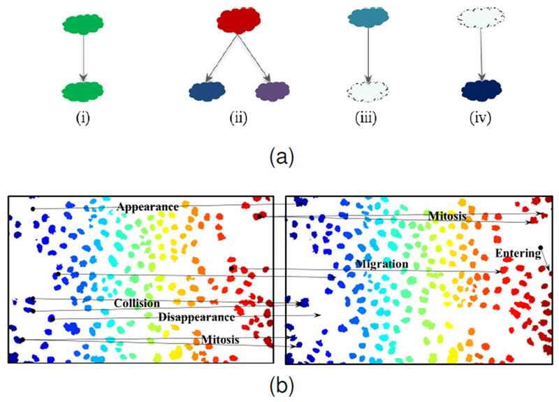
(a) Association cases considered in our tracking system (i) migration, (ii) mitosis, (iii) disappearance, or apoptosis, or leaving field of view, and (iv) appearance, or cells entering the field of view. (b) Examples of cell events occurring in two consecutive sample frames of N2DL-Hela2 dataset.
Our tracking system produces the following data and information: globally linked cell indicator maps, the cell lineage tree, and the tracking output measurements providing the birth and death information, the mitosis events, and quantitative cell measures.
2.1. Pre-tracking
Given the cell indicator maps of an image sequence, we apply a pre-tracking stage to reduce the false positives in cell detection and over- and under-segmentation of cells. We first apply a decision threshold to distinguish between cell and non-cell regions in the cell indicator map. This value is determined by the minimum cell area for an object to be considered as a cell or part of the background. This procedure aims to remove the non-cell detected objects before tracking in order to reduce the false positives.
On the other hand, in datasets of high cell density, the cells can be so close that they can be falsely detected and segmented as a single cell leading to false negatives as shown in Fig. 3. In this case, we split clusters of multiple cells using geometrical shape priors, distance transform on the watershed relief, and the H-minima transform [36].
Fig. 3.

Examples of clusters of cells detected as a single cell before pre-tracking.
To separate fused cells, we apply watershed segmentation to the signed Euclidean distance map D, computed on the cell segmentation map B, so that D = DT(B), where DT denotes the signed distance transform. This operation creates a boundary between the different cells in the cluster. The watershed transform has been proposed by many authors for nuclei segmentation [37], [38]. However, the number of peaks in the distance map may result in over-segmentation by splitting the clusters of cells into more regions than necessary. To reduce the number of over-segmented cell fragments and reduce spurious local minima, we use a morphological reconstruction technique that is the H-minima transform. H-minima Transform [36], [39] is a morphological operation obtained by erosion of the image D increased by a height h defined by
| (1) |
where Rϵ is defined as the reconstruction by erosion morphological operator and h is a depth parameter. H-minima transform removes spurious local minima and avoids over-segmentation by supressing all the regional minima whose depth is smaller than h. H-minima/maxima transform has been largely used in nuclei detection in biomedical images [40], [41].
As an example, we show in Fig. 4 a binary cell mask B, the cell label map L, the cell boundaries before cell separation, the distance map D, the watershed map obtained from the reconstructed distance map after H-minima transform H, and finally the corresponding watershed regions depicting the separated cells.
Fig. 4.
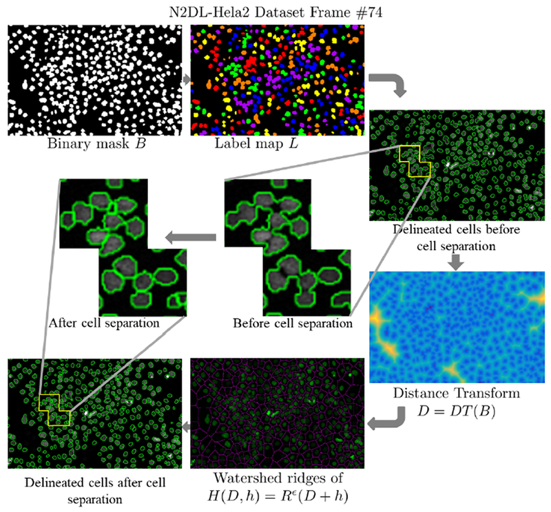
Stage-wise example of cell cluster separation on frame #74 of N2Dl-Hela02 dataset. The magnified parts of the image show the delineated cells before and after separation.
2.2. Estimating Cell Motion
We estimate the motion of each cell in a specific frame and predict the cell locations in the next frame prior to cell matching. This is a challenging task mainly because of potential limitations in temporal resolution, and variable types of cell motion. For example, the biological cells may follow a Brownian movement, which makes the motion estimation very hard. Next, we outline the principles and limitations of conventional optical flow computation and describe the combined local/global optical optical flow (CLGOF) technique that we utilize to address limitations of the conventional techniques.
2.2.1. Optical Flow Computation
The optical flow estimates the velocity of each pixel between two consecutive frames at times t and t+Δt based on spatio-temporal image intensity variations. This method is used in computer vision to characterize and quantify the motion of objects.
Methods for optical flow estimation are based on the computation of partial derivatives of the image intensities signal. Two fundamental techniques were proposed in [42] and [43]. Lucas and Kanade [42] proposed a local method that uses a spatial constancy assumption. The method by Horn and Schunk [43] is a global method that supplements the optical flow constraint with a regularizing smoothness term.
In the computation of optical flow we usually make implicit or explicit assumptions that set constraints to the problem. We assume gradual changes of image motion of an object. That is, the image motion slowly changes in time. In practice, this means the temporal increments are fast enough compared to the motion of objects in a frame. In this case, the temporal difference approximates the derivative of the intensity with respect to time. An additional constraint is that of spatial smoothness that requires neighboring pixels to have approximately the same motion. Finally, we may assume that the gradient of the image intensities is not changed by the displacement.
Local optical flow estimation techniques enable to overcome the aperture problem, where Lucas and Kanade assumed that the optical flow is constant within a neighborhood determined by an integration scale ρ. The integration scale is produced by convolution with a Gaussian kernel Kρ with standard deviation equal to ρ. They proposed to use a least square fitting method to solve the linear system in equation (2) and estimate the optical flow components (u, v)T [42]:
| (2) |
where Ix, Iy, It denote the pixel intensity derivatives along the x-, y- and temporal directions respectively. Because we cannot find solutions at all points, the resulting field is non-dense. Therefore an interpolation step is used to alleviate this shortcoming.
Another category of approaches perform global estimation to produce a dense flow field by minimizing a global functional with regularization constraints. Horn and Schunk [43] proposed to find the field (u, v)T as the minimizer of the following functional:
| (3) |
where λ is a Lagrangian multiplier for imposing smoothness constraints to the optical flow field.
The solution of these diffusion-reaction equations is unique. Moreover, at locations where |∇I| ≈ 0, the local flow cannot be computed but the regularization term provides an estimate based on neighboring pixels. Therefore this technique yields a flow estimate for the complete image domain and no interpolation is needed. However global differential methods may be more sensitive to noise than the local techniques. Flow fields are less regularized at noisy image regions because noisy regions are characterized by high gradients that overcome the smoothness regularization term.
2.2.2. Combined Local/Global Optical Flow Method (CLGOF)
The estimated vector fields of the local techniques may not be dense or may have many discontinuities [42], [44], while the global techniques solutions may not be robust [43], [44]. To overcome these drawbacks, we adopt a solution that combines the local and global optical flow estimation principles [44], [45].
The energy functional includes data and smoothness terms. The data term measures the deviations from the intensity constancy assumption and the gradient constancy assumption and is given by:
| (4) |
where , , and γ denotes a parameter that regulates the effect of each deviation on the data term. A function Ψ(s2) may be applied to the integrand to moderate the effect of outliers. We adopt the approach in [44] that utilizes the form of with ϵ = 0.001. The data term expression becomes:
| (5) |
The purpose of the smoothness term is to penalize discontinuities of the optical flow field and is given by:
| (6) |
where ∇ST = (∂x, ∂y, ∂t)T is the spatiotemporal gradient.
The joint energy functional is:
| (7) |
Based on the calculus of variations, the minimizer of equation (7) is a solution of the Euler-Lagrange equations:
| (8) |
where , , , , , , , . Reflecting boundary conditions are utilized to solve the system of equations in (8).
This technique yields an approximation of the displacement field :
| (9) |
The displacement field solution is first estimated on a coarse grid of the image plane produced by downsampling, and then on the original grid. This multi-scale approach yields a more accurate global solution than a single-scale approach because it reduces false convergence to local minima of the energy functional. The final solution found at the coarse scale is used to initialize the finer scale [45]. An example of the optical flow estimate during cell division using this method is displayed in Fig. 5.
Fig. 5.
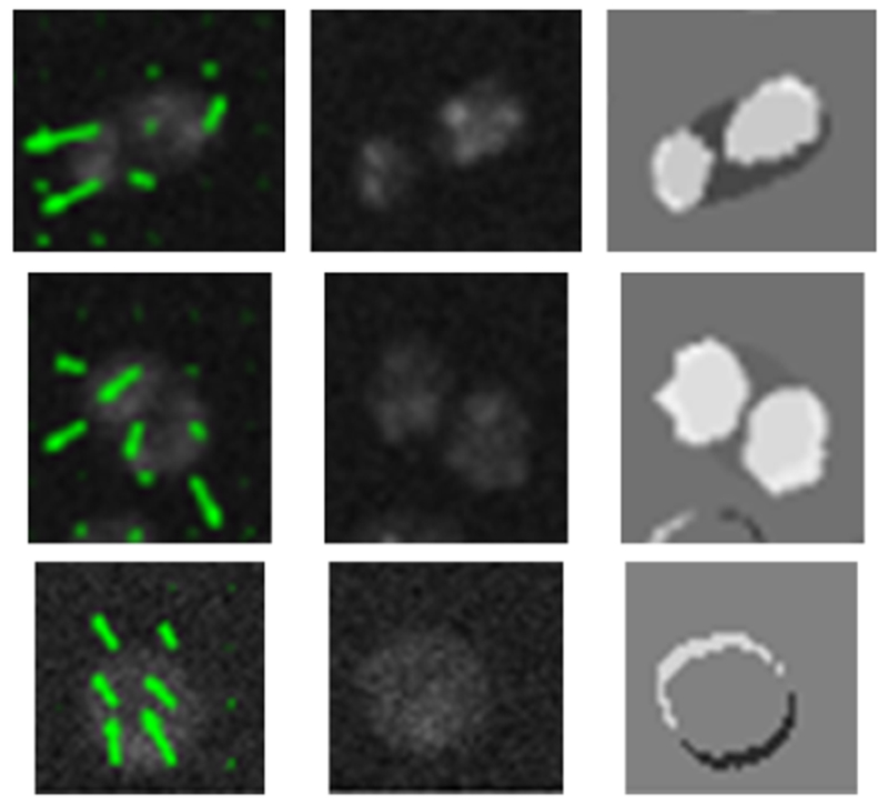
CLGOF estimate indicated by green arrows showing cell mitosis (first and second row), and cell displacement (third row) between frames 8 (first column) and 9 (second column). The third column displays the difference between cell indicator functions for frames 8 and 9 of N2DH-SIM05 dataset.
2.3. Applying Motion Field to Previous Cell Indicator Frame
The estimated displacement field is used to calculate a warped frame by:
| (10) |
We define a cell indicator function that maps pixel values onto unique cell identifiers produced by the cell segmentation stage. We apply warping to the cell indicator frame to find before linking the current and previous frame:
| (11) |
The cell matching and linking stage is applied between the pairs of frames and using probabilistic decision functions. An example of the optical flow calculation and application for warping is displayed in Fig. 6.
Fig. 6.
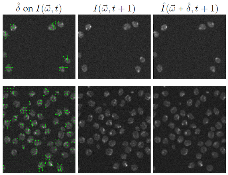
Estimation of vector field displayed on current frame (left), next frame (middle) and warped frame using estimated to be used for cell matching (right). Top row: t = 10 of N2DH-SIM05 dataset. Bottom row: t = 41 of N2DH-SIM04 dataset.
2.4. Likelihood-based Bi-frame Cell Matching
The problem of finding the association with the highest probability is performed by computing the max-likelihood matching for each cell of the current frame among all the cells of the previous warped frame. We formulate bi-frame cell matching as a classification problem.
Let be the states of a system with n cells at time t, be the set of observations for all cells at time t, and be the set of samples for all cells at time t. We also assume a Markov process such that the transition probability depends only on the state of the mother cell or the same cell in previous frame P(St+1|St). We compute the likelihood that the cell i in frame t + 1 is connected with cell j in frame t. Assuming that each cell i in frame t corresponds to a state of nature , we calculate:
| (12) |
Here we define a likelihood function based on the observations derived from the computed cell features. We currently use spatial proximity between cells of warped indicator function and cells of the current indicator function L(ω,t) to form the observation vectors , . Hence
| (13) |
We make a decision using a maximum-a-posteriori (MAP) rule that becomes a maximum likelihood (ML) rule assuming equal priors. We also use a reject option to model cell appearance when the maximum likelihood is still very low. Fig. 7 displays the cell matching procedure including cases of cell appearance, disappearance, and migration.
| (14) |
Fig. 7.
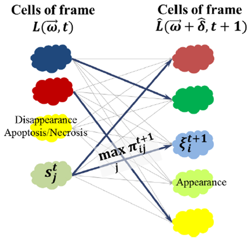
Example of possible cell association likelihood values between cells of warped frame at t + 1 and previous frame at t. The maximum likelihood matches are displayed in bold. The reject option yields the newly appearing cell that has no match with previous frame.
After making a decision we assign the predicted cell class to the cell indicator map .
2.5. Creating Cell Tracks and Acyclic Graph
Overall, the tracking and cell detection problem can be viewed as a partitioning problem by cost minimization. We first introduce the framework for cell track representation, construction, and optimization.
Definition 2.1 (Cell track set). Let N be the number of frames in a time-lapse sequence, and M be the total number of cell tracks. We define the global set of cell labels among all the frames as and the set of all cell tracks in a sequence as ΦM, such that |ΦM| = M.
Definition 2.2 (Individual cell track). We define each track ϕi ∈ ΦM as the set of identified cell states in the sequence.
| (15) |
where tstart and tend denote the first and last frame of the track in the sequence with 0 ≤ tstart ≤ tend ≤ N − 1.
Cell tracking optimization problem –
Our goal is to identify all cell tracks ΦM in the sequence. This can be formulated as follows: Let be the cost computed over a specific track set ΦM.
Find cell track set
| (16) |
with the conditions
| (17) |
| (18) |
After finding a solution , we assign a track label l ∈ LG to each cell. The track duration is defined from the discrete time point of cell appearance till its disappearance, division, or reaching the end of sequence. If a new cell appears, then we create a new track. In the case of cell division we end the track of the mother cell and create two new daughter tracks.
2.5.1. Creating Cell Tracks
First, we create linked lists of the cell states that map each cell to its best match. This is accomplished by pairing each cell of the warped label map at time t with one cell in the label map at time tp using the maximum likelihood approach described in Section 2.4.
Next, we use the created linked lists to construct the cell tracks. We traverse the set of cell states in reverse chronological order and we store the cell track information in a cell track array structure. The elements of this structure are quadruples , that contain the frame id t, cell label (indicator) id , previous frame id tp, and previous label id . This procedure is outlined in Algorithm 1.
The previous procedure produces a cell track structure that holds the tracks ϕi and addresses cell appearance and disappearance. However, at the end of this stage some tracks may be partially overlapping that is in the case of cell division, where different cells have a common ancestor. We address these cases by finding the overlapping parts of two tracks ϕj and ϕk, and creating three new tracks, one for the parent ϕp = ϕj∩ϕk, and the 2 daughters ϕq = ϕj−(ϕj ∩ ϕk) and ϕr = ϕk − (ϕj ∩ ϕk). This procedure is outlined in Algorithm 2.
Algorithm 1.
Construct cell tracks
| Require: Cell_Linked_Lists |
| 1: for each linked list in Cell_Linked_Lists from end to beginning of list do |
| 2: for each cell in linked list do |
| 3: if , k = 1, …, m previous track then |
| 4: set m ← m + 1, create a new track ϕm in Cell_Track_Structure |
| 5: repeat |
| 6: find matching cell label in previous frame recursively in Cell_Linked_Lists |
| 7: add to Cell_Track_Structure |
| 8: until end of current linked list |
| 9: end if |
| 10: end for |
| 11: end for |
| 12: return |
Algorithm 2.
Identify and handle cell events
| Require: |
| 1: for each track ϕi ∈ ΦM do |
| 2: while there exists a previous match of such that do |
| 3: search for in Cell_Track_Structure and find matches |
| 4: if new match is found then |
| 5: if , k = i + 1, …, M then |
| 6: {division is detected; form three new tracks; parent ϕp, and 2 daughters ϕp, ϕr} |
| 7: ϕp = ϕi ∩ ϕk′, |
| 8: ϕq = ϕi − (ϕi ∩ ϕk), ϕr = ϕk − (ϕi ∩ ϕk) |
| 9: {update cell track set} ΦM+1 ← (ΦM − {ϕi, ϕk}) ∪ {ϕp, ϕq, ϕr} |
| 10: else if cell is only in previous tracks then |
| 11: close track ϕi and set parent label to 0 |
| 12: end if |
| 13: else |
| 14: {migration is detected} add cell to existing track; . |
| 15: end if |
| 16: end while |
| 17: end for |
| 18: return |
2.5.2. Minimal Cost Cell Labeling
The individual maximum likelihood tracks ϕi constistute minimum error solutions according to Bayesian theory [46]. Therefore, the proposed algorithm can be considered as a forest of minimal cost chains with temporal constraints that minimizes the cost in the universe of cell tracks Φ defined as:
| (19) |
where C(ϕi) is the total cost of the cell track ϕi.
| (20) |
where c : ℝ → ℝ is a decreasing function of sigmoid or exponential form. Our approach outlined in Algorithm 1 determines a greedy solution to this combinatorial optimization problem. The cell event analysis described in Algorithm 2 ensures that the solution set is non-overlapping and exhausts the universe of cell tracks for each sequence.
2.5.3. Representing Cell Tracks using an Acyclic Oriented Graph
Cell tracking results can be represented using an acyclic oriented graph. The nodes of such a graph correspond to the detected cells, whereas its edges coincide with temporal relations between them. The acyclic graph G = (V, E) consists of a vertex set V and an edge set E such that E ⊂ V × V. The condition for an ordered vertex pair to belong to the edge set E is:
| (21) |
The function P : Ξ → Ξ, where Ξ is the universe of cell states ξi, returns the parent ξa of an entity ξi that is ξa = P(ξi). The first case of an edge in equation (21) represents cell migration, while the second case represents cell division. The graph is guaranteed to be acyclic because the edges are oriented and they follow the ascending temporal ordering of the cell state indicators within and between tracks.
We create an acyclic graph table by traversing the processed cell trajectories that were formed by the Algorithm 2 to find last frame, first frame, and parent track id. Finally we create an adjacency list of the graph nodes and sort and relabel the nodes to create a tree representation. We write the adjacency list to file and plot the constructed acyclic graph using node color coding that indicates the cell states of appearance, migration, division, and disappearance as displayed in Fig. 9. Finally, we assign graph node labels LG(V) to cells in each indicator image and create a global indicator function FL : Ω → LG represented by a 2D+t label structure.
Fig. 9.
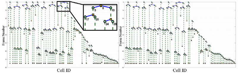
Cell lineage trees automatically generated by our method on Fluo-N2DH-SIM06 dataset using manual cell segmentation and automated tracking (left) and fully automated cell segmentation and tracking (right).
3. Cell Tracking Experiments
In our work, cells are first detected and delineated in all the frames of the sequence independently from the tracking method. The tracking is done sequentially throughout the whole time-lapse sequence, and each cell of each frame is paired to none, one or two cells of the next frame. We track the cells by associating the segmented cell regions and making connections to accurately handle physiological cell events that take place during the course of the imaging experiment.
In this section, we describe the cell tracking experiments including the validation against reference data for tracking and we discuss the results. In addition, we display and discuss the cell lineage trees, the detected cell trajectories, and cell quantification results.
The ground truth data for tracking consist of images with markers and a directed acyclic graph for each image sequence. To evaluate tracking accuracy we utilize a graph matching cost function that we describe next.
3.1. Tracking Evaluation
The tracking accuracy measure symbolized by TRA aims to evaluate the capability of an automated algorithm to detect and track cells versus reference tracking data that were described in [18]. TRA calculates the difference between the acyclic oriented graph produced by the tested method and the TRA-GT-F reference graph [47]. TRA calculates the least number of graph operations needed in order to transform the test graph produced by the tested method to TRA-GT-F.
The TRA measure is given by
| (22) |
In this equation, TRAP is the weighted sum of the graph matching operations of node splitting, node adding, node deletion, edge deletion, edge addition and edge semantics editing. TRAE denotes the cost of constructing the reference graph from the beginning. TRAE is given by
| (23) |
In this equation, |M| denotes the cardinality of the node set, and |E| denotes the cardinality of the link set of TRA-GT-F. The division operation in equation (22) normalizes the graph cost, and the subtraction from 1 defines an evaluation function that increases with better tracking, such that TRA ∈ [0, 1]. Because the acyclic oriented graphs represent the cells, their states, and the associated cell events, TRA also quantifies the capability of an algorithm for automated cell event detection.
3.2. Automated Cell Tracking Results
The objective of cell tracking is to identify and follow the segmented cells in a time-lapse sequence. We performed cell tracking experiments and validated them against reference tracking results using the TRA measure. We then computed and visualized the cell lineage trees produced by the automated tracking algorithm. We finally computed static and dynamic cell measures.
We validated our tracking approach in two stages; first we used cell segmentation maps that were manually generated by the organizers of the IEEE ISBI Cell Tracking Challenge that we denote by CTC [48]. Then, we tested our fully automated cell segmentation and tracking system that includes our cell segmentation method denoted by ST-Diff-TCV [33].
3.2.1. Experiment 1: Tracking validation using reference segmentation
Table 1 lists the tracking accuracy measure denoted by TRAGT and calculated by equation (22) using as input the manual cell segmentation masks denoted by GT for the ground truth. In Table 1, we observe that the tracking method produces very high accuracy rates with an average of 0.992. These results show that our tracking approach is able to detect cell events very efficiently given a reference segmentation. It was able to detect cell migration, mitosis, appearance and disappearance events that occur in the test sequences. We note that when we use the reference label maps, the tracking performance level is about the same for simulated and real sequences.
TABLE 1.
TRA values obtained from our automated tracking applied to reference segmentation masks.
| Dataset name | Size | Number of Frames | TRAGT |
|---|---|---|---|
| N2DH-SIM01 | 494x534 | 56 | 0.999 |
| N2DH-SIM02 | 569x593 | 100 | 0.998 |
| N2DH-SIM03 | 606x605 | 100 | 0.997 |
| N2DH-SIM04 | 673x743 | 56 | 0.999 |
| N2DH-SIM05 | 597x525 | 76 | 0.988 |
| N2DH-SIM06 | 655x735 | 76 | 0.997 |
| C2DL-MSC01 | 992x832 | 48 | 0.999 |
| C2DL-MSC02 | 1200x782 | 48 | 0.973 |
| N2DL-HeLa01 | 1100x700 | 92 | 0.992 |
| N2DL-HeLa02 | 1100x700 | 92 | 0.970 |
| N2DH-GOWT101 | 1024x1024 | 92 | 0.998 |
| N2DH-GOWT102 | 1024x1024 | 92 | 0.996 |
Even when reference segmentation is given, tracking by itself presents certain challenges. Microscopy live cell image sequences may have temporal and spatial resolution limitations and cell may move at variable speeds thus complicating the motion analysis and matching stages. Computing the displacement field between each two pairs of frames using the CLGOF method before our bi-frame matching, enables us to successfully overcome the problem of large time and space discrepancies for a robust and efficient cell tracking system.
3.2.2. Experiment 2: Tracking validation of fully automated tracking methodology
Next, we validated our joint automated segmentation and tracking methodology that employs our ST-Diff-TCV segmentation method [33] to delineate the cells prior to tracking. We denote our fully automated tracking method by ST-Diff-TCV-Tr. Table 2 displays the tracking validation results as TRA values along with the segmentation accuracy expressed by Dice Similarity Coefficient (DSC) values. Overall, our method produces very promising tracking rates with an average tracking rate TRA of 0.891. We note that the segmentation stage, which yields average DSC of 0.893, allows for efficient tracking detection. In specific cases, over- or under-segmentation of a cell may significantly reduce the tracking accuracy. The lower TRA value for the C2DL-MSC02 sequence is caused by the very low contrast-to-noise-ratio and signal-to-noise-ratio characteristics of this sequence and very elongated cell morphology with high intensity variability inside the cell body. These effects result in over-segmentation, which creates false positives in cell detection and tracking. In addition, under-segmentation produces false negatives in cell detection that are propagated to the tracking stage. In the N2DL-HeLa sequences some clustered cells were not delineated correctly, resulting in under-segmentation that reduced the tracking accuracy. Cell segmentation errors also occurred in C2Dl-MSC sequences because the cells have elongated shapes and variable levels of intensity in different parts of each cell resulting also in low contrast. On the other hand, ST-Diff-TCV-Tr tracking performed very well for N2DH-GOWT sequences even though they include several challenges such as heterogeneous average cell intensities and unlabeled cell nucleoli. Our results support the premise that tracking is dependent on segmentation.
TABLE 2.
TRA and DSC values obtained from our automated joint segmentation and tracking method denoted by ST-Diff-TCV-Tr.
| Dataset | DSC (μ ± σ) | TRA |
|---|---|---|
| N2DH-SIM01 | 0.926 ± 0.050 | 0.963 |
| N2DH-SIM02 | 0.942 ± 0.012 | 0.949 |
| N2DH-SIM03 | 0.939 ± 0.027 | 0.964 |
| N2DH-SIM04 | 0.934 ± 0.013 | 0.964 |
| N2DH-SIM05 | 0.941 ± 0.014 | 0.940 |
| N2DH-SIM06 | 0.960 ± 0.026 | 0.973 |
| C2DL-MSC01 | 0.762 ± 0.034 | 0.853 |
| C2DL-MSC02 | 0.805 ± 0.043 | 0.584 |
| N2DL-HeLa01 | 0.825 ± 0.042 | 0.816 |
| N2DL-HeLa02 | 0.865 ± 0.005 | 0.845 |
| N2DH-GOWT101 | 0.903 ± 0.012 | 0.913 |
| N2DH-GOWT102 | 0.918 ± 0.010 | 0.914 |
3.2.3. Comparisons with Other Methods
Here we compare the performance of our fully automated tracking method ST-Diff-TCV-Tr with cell tracking methods developed by research groups that participated in previous Cell Tracking Challenges and were published in [18], [47]. In our comparisons we included methods that produced the top 3 overall tracking measures over our test data in CTC. These methods are denoted by KTH-SE, IMCB-SG_1, and UP-PT. KTH-SE includes 3 algorithms using bandpass [18], variance, or ridge segmentation and performs track linking based on the Vitterbi algorithm [27]. IMCB-SG_1 finds seeds using the extended maxima transform and applies seed-controlled watershed for cell segmentation. Tracking is accomplished by linking seeds between frames. UP-PT uses a local interest point detector for cell detection and applies Euclidean distance-based nearest neighbor search to SIFT descriptors for tracking [17]. Furthermore, we included results from the methods FR-Ro-GE and HD-Har-GE that have produced top ranked TRA values for specific sequences as described in [47]. FR-Ro-GE uses convolutional neural networks for segmentation [19] and greedy label propagation for tracking. The authors proposed a fully convolutional network (fCNN) architecture that they denoted as the U-net that includes an upsampling stage. The utilization of deep learning technique implies very good segmentation results, however tracking was not successful for the N2DH-GOWT1 sequences. HD-Har-GE utilizes thresholding and watershed transformation for segmentation and local spatio-temporal optimization for tracking [49]. We also included the average performance by the top 3 methods of CTC KTH-SE, IMCB-SG_1, and UP-PT denoted by CTC_T3, and the average performance of all 21 participants of CTC (denoted by CTC_ALL). The latter measure may be used to compare the performance of individual methods to the average level of competition in the CTC challenge.
Table 3 contains the TRA scores for all methods over each subset of the tested image sequences. We observe that our method ST-Diff-TCV-Tr yields significantly better tracking rates than CTC_ALL for each sequence. Also, it produces higher TRA scores than the average TRA of the top 3 methods -denoted by CTC_T3. When compared to individual methods, ST-Diff-TCV-Tr produces higher TRA rates than 4 of the 5 methods that had stood out in CTC challenges.
TABLE 3.
Comparisons between tracking performance values over all the tested image sequences.
| TRA | |||||
|---|---|---|---|---|---|
| Method | N2DH-SIM | C2DL-MSC | N2DL-HeLa | N2DH-GOWT1 | μ ± σ |
| FR-Ro-GE | 0.975 | 0.691 | 0.976 | - | 0.661 ± 0.399 |
| HD-Har-GE | 0.703 | 0.589 | 0.986 | 0.906 | 0.796 ± 0.206 |
| IMCB-SG_1 | 0.907 | 0.633 | 0.915 | 0.882 | 0.834 ± 0.131 |
| KTH-SE | 0.957 | 0.763 | 0.991 | 0.976 | 0.922 ± 0.107 |
| UP-PT | 0.896 | 0.478 | 0.972 | 0.875 | 0.805 ± 0.208 |
| CTC_ALL | 0.526 | 0.277 | 0.595 | 0.516 | 0.478 ± 0.139 |
| CTC_T3 | 0.920 | 0.625 | 0.959 | 0.911 | 0.854 ± 0.154 |
| ST-Diff-TCV-Tr | 0.959 | 0.719 | 0.831 | 0.914 | 0.856 ± 0.105 |
In Fig. 8 we display the summarized TRA rates for each of the compared methods over all the datasets. We note that the average tracking performance of our method is competitive with the top 3 methods from CTC. These results show that our method produces very good levels of accuracy for each set and on average. While the KTH-SE method is the only method that yields higher average tracking performance than ST-Diff-TCV-Tr, it requires selection of segmentation algorithm for each sequence [47], therefore it may not be considered as a fully automated method and may not be directly comparable with the other methods.
Fig. 8.
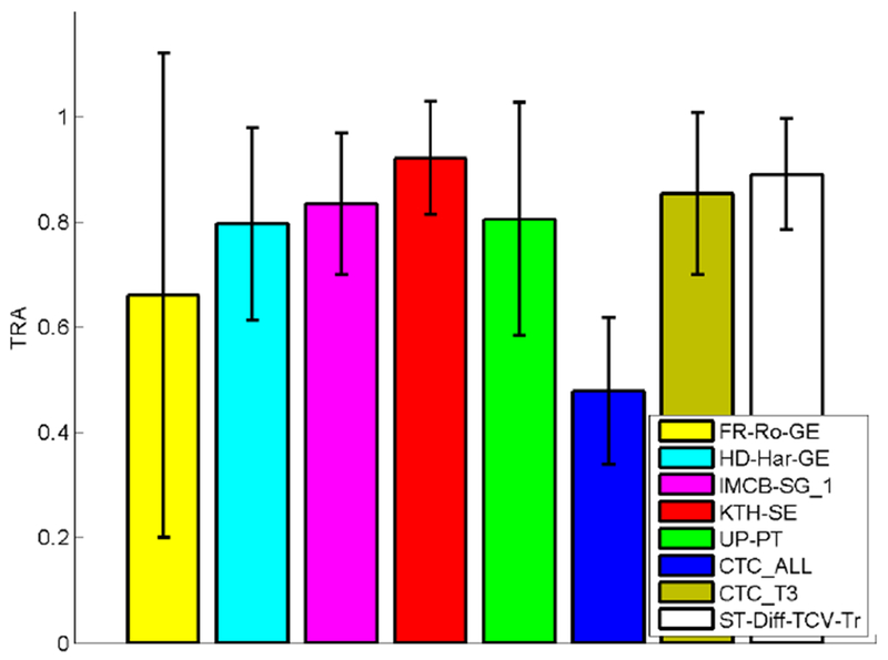
Comparisons between tracking performance values over all the tested image sequences.
We also performed paired t-tests between the TRA scores of ST-Diff-TCV-Tr and the scores produced by each one of the other methods. The test versus CTC_ALL produced a p value of 4.3 × 10⁻⁵ indicating that the tracking performance improvement of ST-Diff-TCV-Tr versus CTC_ALL is statistically significant. All other p-values were greater than 0.05.
3.3. Visualization of Cell Trajectories
The tracking accuracy measure TRA that was defined in equation (22), computes the similarity between lineage trees identified by our methodology versus reference lineage trees that were constructed manually by human operators.
We illustrate in Fig. 9 the cell lineage trees automatically generated by our tracking approach using the reference cell identifier maps (left) and our automated cell segmentation results (right) for a simulated sequence that includes numerous mitosis events. The two trees in this example have very similar structure that implies high TRA for both methods. Indeed, TRAGT = 0.997 and TRA = 0.973. Furthermore, Fig. 10 displays the cell lineage tree produced by our fully automated cell segmentation and tracking methodology on a dense real test sequence of HeLa cells. A cell lineage tree in general corresponds to the directed acyclic graph. It represents and visualizes the tracked cells and the cell events detected by our tracking methodology. More specifically, our automatically constructed cell lineage trees CLT(V, E) consist of nodes V that represent the cells that are identified across the sequence, and links E that represent the cell event evolution, namely cell migration, cell appearance and disappearance, and cell mitosis. The dashed links denote cell migration and the continuous links denote a parent-daughter relationship.
Fig. 10.
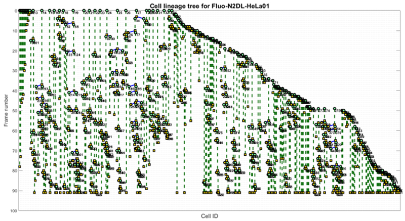
Cell lineage tree generated by our fully automated method on the dense dataset Fluo-Hela01 dataset. This case yields TRA=0.816.
As an application of cell tracking, we generated cell trajectories in the projected 2D domain in Fig. 11a and in the 2D+t domain displayed in Fig. 11b. The system produces automatically the cell trajectory graphs using the global cell indicator functions. In these figures the trajectories are color-coded and each color represents the biological events during the lifetime of a single cell. The track IDs are also displayed next to the end of each cell trajectory for reference. The cell trajectories can effectively provide a visual analysis tool of a biological experiment. More specifically, they reveal mother and daughter relations, and metrics such as symmetry and division times can be extracted from cell lineage. Types of motion can also be visually inferred from the 2D projections of trajectories. Straightforward applications include the development of predictive models for stem cell population growth and design, and optimization of subcultural strategies.
Fig. 11.
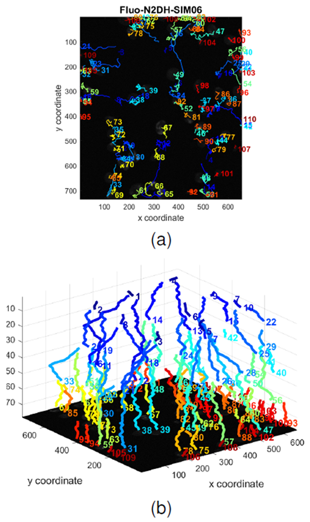
Cell tracks in 2D, 2D+t automatically generated by our method on Fluo-N2DH-SIM06 dataset.
3.4. Cell Quantification
A significant application of tracking is cell quantification and quantitative analysis. Quantification is the computation of biologically meaningful cell measures that can be divided into morphological, motility, diffusivity, and velocity measures. Morphological measures include the area, perimeter, and shape features such as the major and minor principal axes geometry, eccentricity, solidity, and convexity. More sophisticated shape features can be computed using Fourier descriptors, Independent Component Analysis (ICA), and Principal Component Analysis (PCA). Motility measures are computed from the trajectories of the tracked cells using piecewise linear approximation. Typical motility measures include the total distance traveled by each cell, the net distance that is the distance between the start and the end points in a trajectory, the total trajectory time, or cell life time. An advanced measure of diffusivity is the Mean Squared Displacement (MSD) that is computed by the second-order moment of displacement as a function of time point difference and is defined as follows
| (24) |
where ωi = (xi, yi) is the centroid of a cell at time point i, N is the total trajectory lifetime, and n is the interval for computation of MSD. A frequent selection for the distance function d(·, ·) is the Euclidean distance d(ωi, ωi+n = ‖ωi − ωi+n‖2. MSD is used for characterizing the mode of cell motion. We can accomplish this by observing the MSD-time curve. Some identifiable modes of cell motion are Brownian, anomalous diffusion, region-confined motion, directed motion, or immobility.
In our method we compute 26 morphological, motility, and diffusivity measures. Fig. 12 illustrates a visualization and quantification example for the sequence Fluo-C2DL-MSC02. Fig. 12a and Fig. 12c display the detected cell trajectories in the projected 2D domain and the 2D+t domain respectively. Fig. 12b and Fig. 12d illustrate the MSD function versus time and the mean MSD value for each cell. In these plots we can identify different motion modes including linear and exponential types. A linear MSD type indicates Brownian motion. A MSD curve approximated by a power law function may indicate superdiffusion, normal diffusion or subdiffusion, depending on the approximated power coefficient value. Our system automatically produces the quantification measures and related plots for all cells and trajectories for an input time-lapse sequence.
Fig. 12.
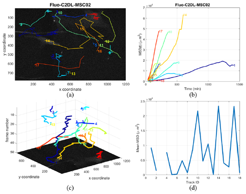
2D and 2D+t displays of all cell trajectories of Fluo-C2DL-MSC02 in (a) and (c), MSD function versus time and the MSD mean over time for each cell of the C2DL-MSC02 dataset in (b) and (d).
4. Conclusion
Our work concentrated on the design, development and validation of an automated cell tracking system. We propose a formulation of cell tracking as an optimization problem of graph partitioning and we introduce a solution in this context. We utilize the predicted cell motion by the multiscale Combined Local-Global Optical Flow technique in a probabilistic decision framework to find inter-frame cell correspondences. This increases the robustness of tracking with respect to temporal sampling limitations of the image sequences and diverse cell motion types. Another contribution of this work is the fully automated cell tracking, lineage construction and quantification system that enables the analysis of very large volumes of data.
We performed extensive experiments for evaluating the performance of our method. Our tracking and event detection technique when applied to reference segmentation maps produces an average TRA measure of 99%, while our fully automated segmentation and tracking method denoted by ST-Diff-TCV-Tr performed at 89%. We performed comparisons to leading-edge cell tracking methods, which indicate that the proposed technique produces very good tracking accuracy relatively to these techniques.
Acknowledgments
The authors would like to acknowledge the support by the Center for Research and Education in Optical Sciences and Applications (CREOSA) in Delaware State University funded by NSF CREST-8763. Research reported in this publication was also supported by the National Institute of General Medical Sciences of the National Institutes of Health under Award Number SC3GM113754. The content is solely the responsibility of the authors and does not necessarily represent the official views of the National Institutes of Health.
Biographies

Fatima Boukari is a Visiting Assistant Professor with the Division of Physical and Computational Sciences in Delaware State University. She earned a PhD in Mathematics and Physics from Delaware State University in 2017. She earned the Engineering degree and Masters degree in Computer Science from University of Annaba, Algeria. Her research interests are image analysis, pattern recognition, and mathematical methods for biomedical applications. She is a member of IEEE, IEEE Women in Science and Engineering, and SPIE.

Sokratis Makrogiannis is an Associate Professor with the Division of Physical and Computational Sciences in Delaware State University. He received the BS in Physics, MS in Electronics and the PhD degree in the area of Image Analysis from University of Patras, Patras, Greece in 1995,1998 and 2002 respectively. He completed post-doctoral training on biomedical image analysis in Univ. of Pennsylvania (2005-2006) and on computer vision in Wright State University (2003-2005). His scientific interests are in the areas of image analysis and pattern recognition with application to biomedicine and computer vision. Prior to DSU he was a senior research fellow in NIH/NIA, and has worked as an imaging scientist/engineer at GE Global Research and GlaxoSmithKline R&D.
Contributor Information
Fatima Boukari, Department of Mathematics, Delaware State University, Dover, DE, 19901.
Sokratis Makrogiannis, Department of Mathematics, Delaware State University, Dover, DE, 19901.
References
- [1].Eils R and Athale C, “Computational imaging in cell biology.” J Cell Biol, vol. 161, no. 3, pp. 477–481, May 2003. [Online]. Available: 10.1083/jcb.200302097 [DOI] [PMC free article] [PubMed] [Google Scholar]
- [2].Stephens DJ and Allan VJ, “Light microscopy techniques for live cell imaging.” Science, vol. 300, no. 5616, pp. 82–86, April 2003. [Online]. Available: 10.1126/science.1082160 [DOI] [PubMed] [Google Scholar]
- [3].Braun KM, Niemann C, Jensen UB, Sundberg JP, Silva-Vargas V, and Watt FM, “Manipulation of stem cell proliferation and lineage commitment: visualisation of label-retaining cells in wholemounts of mouse epidermis,” Development, vol. 130, no. 21, pp. 5241–5255, 2003. [Online]. Available: http://dev.biologists.org/content/130/21/5241 [DOI] [PubMed] [Google Scholar]
- [4].Boukari F, Makrogiannis S, Nossal R, and Boukari H, “Imaging and tracking hiv viruses in human cervical mucus,” Journal of Biomedical Optics, vol. 21, no. 9, pp. 096 001-1–096001-7, 2016. [Online]. Available: 10.1117/1.JBO.21.9.096001 [DOI] [PMC free article] [PubMed] [Google Scholar]
- [5].Zimmer C, Labruyere E, Meas-Yedid V, Guillen N, and Olivo-Marin J-C, “Segmentation and tracking of migrating cells in videomicroscopy with parametric active contours: a tool for cell-based drug testing.” IEEE Trans Med Imaging, vol. 21, no. 10, pp. 1212–1221, October 2002. [Online]. Available: 10.1109/TMI.2002.806292 [DOI] [PubMed] [Google Scholar]
- [6].Ray N, Acton ST, and Ley K, “Tracking leukocytes in vivo with shape and size constrained active contours.” IEEE Trans Med Imaging, vol. 21, no. 10, pp. 1222–1235, October 2002. [Online]. Available: 10.1109/TMI.2002.806291 [DOI] [PubMed] [Google Scholar]
- [7].Padfield D, Rittscher J, Thomas N, and Roysam B, “Spatio-temporal cell cycle phase analysis using level sets and fast marching methods.” Med Image Anal, vol. 13, no. 1, pp. 143–155, February 2009. [Online]. Available: 10.1016/j.media.2008.06.018 [DOI] [PubMed] [Google Scholar]
- [8].Padfield D, Rittscher J, and Roysam B, “Coupled minimum-cost flow cell tracking for high-throughput quantitative analysis.” Med Image Anal, vol. 15, no. 4, pp. 650–668, August 2011. [Online]. Available: 10.1016/j.media.2010.07.006 [DOI] [PubMed] [Google Scholar]
- [9].Dufour A, Thibeaux R, Labruyere E, Guillen N, and Olivo-Marin J-C, “3-d active meshes fast discrete deformable models for cell tracking in 3-d time-lapse microscopy,” IEEE transactions on image processing, vol. 20, no. 7, pp. 1925–1937, July 2011, iEEE Transactions on Image Processing. [DOI] [PubMed] [Google Scholar]
- [10].Mukherjee DP, Ray N, and Acton ST, “Level set analysis for leukocyte detection and tracking.” IEEE Trans Image Process, vol. 13, no. 4, pp. 562–572, April 2004. [DOI] [PubMed] [Google Scholar]
- [11].Zhang B, Zimmer C, and Olivo-Marin JC, “Tracking fluorescent cells with coupled geometric active contours,” in Proc. 2nd IEEE Int. Symp. Biomedical Imaging: Nano to Macro (IEEE Cat No. 04EX821), vol. 1, Apr. 2004, pp. 476–479. [Google Scholar]
- [12].Dufour A, Shinin V, Tajbakhsh S, Guillén-Aghion N, Olivo-Marin J-C, and Zimmer C, “Segmenting and tracking fluorescent cells in dynamic 3-d microscopy with coupled active surfaces.” IEEE Trans Image Process, vol. 14, no. 9, pp. 1396–1410, September 2005. [DOI] [PubMed] [Google Scholar]
- [13].Li F, Zhou X, Ma J, and Wong STC, “Multiple nuclei tracking using integer programming for quantitative cancer cell cycle analysis,” IEEE Transactions on Medical Imaging, vol. 29, no. 1, pp. 96–105, January 2010. [DOI] [PMC free article] [PubMed] [Google Scholar]
- [14].Chenouard N, Bloch I, and Olivo-Marin J-C, “Multiple hypothesis tracking for cluttered biological image sequences.” IEEE Trans Pattern Anal Mach Intell, vol. 35, no. 11, pp. 2736–3750, November 2013. [Online]. Available: 10.1109/TPAMI.2013.97 [DOI] [PubMed] [Google Scholar]
- [15].Smal I and Meijering E, “Quantitative comparison of multiframe data association techniques for particle tracking in time-lapse fluorescence microscopy.” Med Image Anal, vol. 24, no. 1, pp. 163–189, August 2015. [Online]. Available: 10.1016/j.media.2015.06.006 [DOI] [PubMed] [Google Scholar]
- [16].Xing F and Yang L, “Robust nucleus/cell detection and segmentation in digital pathology and microscopy images: A comprehensive review,” IEEE Reviews in Biomedical Engineering, vol. 9, pp. 234–263, 2016. [DOI] [PMC free article] [PubMed] [Google Scholar]
- [17].Esteves T, Oliveira MJ, and Quelhas P, “Cancer cell detection and tracking based on local interest point detectors,” in Image Analysis and Recognition, Kamel M and Campilho A, Eds. Berlin, Heidelberg: Springer Berlin Heidelberg, 2013, pp. 434–441. [Google Scholar]
- [18].Maska M, Ulman V, Svoboda D, Matula P, Matula P,Ederra C, Urbiola A, Espana T, Venkatesan S, Balak DMW, Karas P, Bolckova T, Streitova M, Carthel C, Coraluppi S,Harder N, Rohr K, Magnusson KEG, Jalden J, Blau HM,Dzyubachyk O, Kizek P, Hagen GM, Pastor-Escuredo D,Jimenez-Carretero D, Ledesma-Carbayo MJ, Munoz-Barrutia A, Meijering E, Kozubek M, and Ortiz-de Solorzano C, “A benchmark for comparison of cell tracking algorithms.” Bioinformatics, vol. 30, no. 11, pp. 1609–1617, June 2014. [Online]. Available: 10.1093/bioinformatics/btu080 [DOI] [PMC free article] [PubMed] [Google Scholar]
- [19].Ronneberger O, Fischer P, and Brox T, “U-net: Convolutional networks for biomedical image segmentation,” in Medical Image Computing and Computer-Assisted Intervention – MICCAI 2015, Navab N, Hornegger J, Wells WM, and Frangi AF, Eds. Cham: Springer International Publishing, 2015, pp. 234–241. [Google Scholar]
- [20].Litjens G, Kooi T, Bejnordi BE, Setio AAA, Ciompi F, Ghafoorian M, van der Laak JA, van Ginneken B, and Sánchez CI, “A survey on deep learning in medical image analysis,” Medical Image Analysis, vol. 42, pp. 60–88, 2017. [Online]. Available: http://www.sciencedirect.com/science/article/pii/S1361841517301135 [DOI] [PubMed] [Google Scholar]
- [21].Xing F, Xie Y, Su H, Liu F, and Yang L, “Deep learning in microscopy image analysis: A survey,” IEEE Transactions on Neural Networks and Learning Systems, pp. 1–19, 2018. [DOI] [PubMed] [Google Scholar]
- [22].Al-Kofahi O, Radke RJ, Goderie SK, Shen Q, Temple S, and Roysam B, “Automated cell lineage construction: a rapid method to analyze clonal development established with murine neural progenitor cells.” Cell Cycle, vol. 5, no. 3, pp. 327–335, February 2006. [DOI] [PubMed] [Google Scholar]
- [23].Yang X, Li H, Zhou X, and Wong S, “Automated segmentation and tracking of cells in time-lapse microscopy using watershed and mean shift,” in Proc. Int. Symp. Intelligent Signal Processing and Communication Systems, Dec. 2005, pp. 533–536. [Google Scholar]
- [24].Liu K, Lienkamp S, Shindo A, Wallingford J, Walz G, and Ronneberger O, “Optical flow guided cell segmentation and tracking in developing tissue,” in IEEE International Symposium on Biomedical Imaging (ISBI), 2014, pp. 298–301. [Online]. Available: http://lmb.informatik.uni-freiburg.de/Publications/2014/LR14 [Google Scholar]
- [25].Bise R, Kanade T, Yin Z, and Huh S. i., “Automatic cell tracking applied to analysis of cell migration in wound healing assay,” in Proc. Annual Int. Conf. of the IEEE Engineering in Medicine and Biology Society, Aug. 2011, pp. 6174–6179. [DOI] [PubMed] [Google Scholar]
- [26].Pulford GW and Scala BFL, “Multihypothesis Viterbi data association: Algorithm development and assessment,” IEEE Transactions on Aerospace and Electronic Systems, vol. 46, no. 2, pp. 583–609, Apr. 2010. [Google Scholar]
- [27].Magnusson KEG, Jalden J, Gilbert PM, and Blau HM, “Global linking of cell tracks using the viterbi algorithm.” IEEE Trans Med Imaging, vol. 34, no. 4, pp. 911–929, April 2015. [Online]. Available: 10.1109/TMI.2014.2370951 [DOI] [PMC free article] [PubMed] [Google Scholar]
- [28].Smal I, Draegestein K, Galjart N, Niessen W, and Meijering E, “Rao-blackwellized marginal particle filtering for multiple object tracking in molecular bioimaging.” Inf Process Med Imaging, vol. 20, pp. 110–121, 2007. [DOI] [PubMed] [Google Scholar]
- [29].Yang X, Li H, and Zhou X, “Nuclei segmentation using marker-controlled watershed, tracking using mean-shift, and kalman filter in time-lapse microscopy,” Circuits and Systems I: Regular Papers, IEEE Transactions on, vol. 53, no. 11, pp. 2405–2414, November 2006. [Google Scholar]
- [30].Meijering E, Smal I, and Danuser G, “Tracking in molecular bioimaging,” IEEE Signal Processing Magazine, vol. 23, no. 3, pp. 46–53, May 2006. [Google Scholar]
- [31].Ettinger A and Wittmann T, “Fluorescence live cell imaging,” Methods in cell biology, vol. 123, pp. 77–94, 2014. [DOI] [PMC free article] [PubMed] [Google Scholar]
- [32].Frigault MM, Lacoste J, Swift JL, and Brown CM, “Live-cell microscopy - tips and tools,” Journal of Cell Science, vol. 122, no. 6, pp. 753–767, 2009. [Online]. Available: http://jcs.biologists.org/content/122/6/753 [DOI] [PubMed] [Google Scholar]
- [33].Boukari F and Makrogiannis S, “Joint level-set and spatio-temporal motion detection for cell segmentation,” BMC Medical Genomics, vol. 9, no. 2, p. 49, August 2016. [Online]. Available: 10.1186/s12920-016-0206-5 [DOI] [PMC free article] [PubMed] [Google Scholar]
- [34].——, “Spatio-temporal level-set based cell segmentation in time-lapse image sequences,” in Advances in Visual Computing, ser Lecture Notes in Computer Science, Bebis G, Boyle R, Parvin B, Koracin D, McMahan R, Jerald J, Zhang H, Drucker S, Kambhamettu C, El Choubassi M, Deng Z, and Carlson M, Eds. Springer International Publishing, 2014, vol. 8888, pp. 41–50. [Google Scholar]
- [35].——, “Spatio-temporal diffusion-based dynamic cell segmentation,” in Bioinformatics and Biomedicine (BIBM), 2015 IEEE International Conference on, November 2015, pp. 317–324. [Google Scholar]
- [36].Qi X, Xing F, Foran DJ, and Yang L, “Robust segmentation of overlapping cells in histopathology specimens using parallel seed detection and repulsive level set,” IEEE Transactions on Biomedical Engineering, vol. 59, no. 3, pp. 754–765, Mar. 2012. [DOI] [PMC free article] [PubMed] [Google Scholar]
- [37].Wählby C, Sintorn I-M, Erlandsson F, Borgefors G, and Bengtsson E, “Combining intensity, edge and shape information for 2d and 3d segmentation of cell nuclei in tissue sections,” Journal of Microscopy, vol. 215, no. 1, pp. 67–76, 2004. [Online]. Available: 10.1111/j.0022-2720.2004.01338.x [DOI] [PubMed] [Google Scholar]
- [38].Cloppet F and Boucher A, “Segmentation of overlapping/aggregating nuclei cells in biological images,” in Proc. 19th Int. Conf. Pattern Recognition, Dec. 2008, pp. 1–4. [Google Scholar]
- [39].Soille P, Morphological Image Analysis: Principles and Applications, 2nd ed. Secaucus, NJ, USA: Springer-Verlag New York, Inc., 2003. [Google Scholar]
- [40].Thirusittampalam K, Hossain MJ, Ghita O, and Whelan PF, “A novel framework for cellular tracking and mitosis detection in dense phase contrast microscopy images,” IEEE Journal of Biomedical and Health Informatics, vol. 17, no. 3, pp. 642–653, May 2013. [DOI] [PubMed] [Google Scholar]
- [41].Jung C and Kim C, “Segmenting clustered nuclei using h-minima transform-based marker extraction and contour parameterization,” IEEE Transactions on Biomedical Engineering, vol. 57, no. 10, pp. 2600–2604, Oct. 2010. [DOI] [PubMed] [Google Scholar]
- [42].Lucas BD and Kanade T, “An iterative image registration technique with an application to stereo vision (ijcai),” in Proceedings of the 7th International Joint Conference on Artificial Intelligence (IJCAI ’81), April 1981, pp. 674–679. [Google Scholar]
- [43].Horn BKP and Schunck BG, “Determining optical flow,” ARTIFICAL INTELLIGENCE, vol. 17, pp. 185–203, 1981. [Google Scholar]
- [44].Brox T, Bruhn A, Papenberg N, and Weickert J, “High accuracy optical flow estimation based on a theory for warping,” in European Conference on Computer Vision (ECCV), ser. Lecture Notes in Computer Science, vol. 3024 Springer, May 2004, pp. 25–36. [Online]. Available: http://lmb.informatik.uni-freiburg.de//Publications/2004/Bro04a [Google Scholar]
- [45].Bruhn A, Weickert J, and Schnörr C, “Lucas/kanade meets horn/schunck: Combining local and global optic flow methods,” International Journal of Computer Vision, vol. 61, no. 3, pp. 211–231, 2005. [Online]. Available: 10.1023/B:VISI.0000045324.43199.43 [DOI] [Google Scholar]
- [46].Duda RO, Hart PE, and Stork DG, Pattern Classification (2Nd Edition). Wiley-Interscience, 2000. [Google Scholar]
- [47].Ulman V, Maska M, Magnusson KEG, Ronneberger O, Haubold C, Harder N, Matula P, Matula P, Svoboda D, Radojevic M, Smal I, Rohr K, Jaldén J, Blau HM, Dzyubachyk O, Lelieveldt B, Xiao P, Li Y, Cho S-Y, Dufour A, Olivo-Marin JC, Reyes-Aldasoro CC, Solis-Lemus JA, Bensch R, Brox T, Stegmaier J, Mikut R, Wolf S, Hamprecht FA, Esteves T, Quelhas P, Demirel Ö Malmström L, Jug F, Tomancák P, Meijering E, Muñoz-Barrutia A, Kozubek M, and de Solor CO, “An objective comparison of cell-tracking algorithms,” Nature Methods, vol. 14, pp. 1141–1152, 2017. [Online]. Available: http://lmb.informatik.uni-freiburg.de/Publications/2017/RBB17 [DOI] [PMC free article] [PubMed] [Google Scholar]
- [48].Cell Tracking Challenge, 2013. [Online]. Available: http://www.grand-challenge.org/
- [49].Schiegg M, Hanslovsky P, Kausler BX, Hufnagel L, and Hamprecht FA, “Conservation tracking,” in 2013 IEEE International Conference on Computer Vision (ICCV), vol. 00, Dec. 2013, pp. 2928–2935. [Online]. Available: doi.ieeecomputersociety.org/10.1109/ICCV.2013.364 [Google Scholar]