Prion-like spreading of Alzheimer’s disease within the brain’s connectome

Abstract

The prion hypothesis states that misfolded proteins can act as infectious agents that template the misfolding and aggregation of healthy proteins to transmit a disease. Increasing evidence suggests that pathological proteins in neurodegenerative diseases adopt prion-like mechanisms and spread across the brain along anatomically connected networks. Local kinetic models of protein misfolding and global network models of protein spreading provide valuable insight into several aspects of prion-like diseases. Yet, to date, these models have not been combined to simulate how pathological proteins multiply and spread across the human brain. Here, we create an efficient and robust tool to simulate the spreading of misfolded protein using three classes of kinetic models, the Fisher–Kolmogorov model, the Heterodimer model and the Smoluchowski model. We discretize their governing equations using a human brain network model, which we represent as a weighted Laplacian graph generated from 418 brains from the Human Connectome Project. Its nodes represent the anatomic regions of interest and its edges are weighted by the mean fibre number divided by the mean fibre length between any two regions. We demonstrate that our brain network model can predict the histopathological patterns of Alzheimer’s disease and capture the key characteristic features of finite-element brain models at a fraction of their computational cost: simulating the spatio-temporal evolution of aggregate size distributions across the human brain throughout a period of 40 years takes less than 7 s on a standard laptop computer. Our model has the potential to predict biomarker curves, aggregate size distributions, infection times, and the effects of therapeutic strategies including reduced production and increased clearance of misfolded protein.

1. Motivation

A major advance in our understanding of the human brain has been the realization that the our brain is organized as a network, both at the physical and at the functional levels [1]. This quiet revolution has been made possible by the parallel development of network theory and medical imaging, in particular by the concept of small-world networks [2]. Methods originating from graph theory are now routinely used to study many aspects of brain function and the prevalent dogma is that the brain operates as an efficiently structured, modular, dynamic network with strongly connected hubs [3]. This network is optimized to rapidly transmit information, but, unfortunately, the concept of fast transport also applies to misfolded proteins that highjack the network to rapidly spread across the brain [4]. Previous work has shown that the eigenmodes of the brain network’s graph Laplacian are correlated to brain atrophy in Alzheimer’s disease [5], and probablistic epidemiological models have been proposed to study transference mechanisms within the network [6].

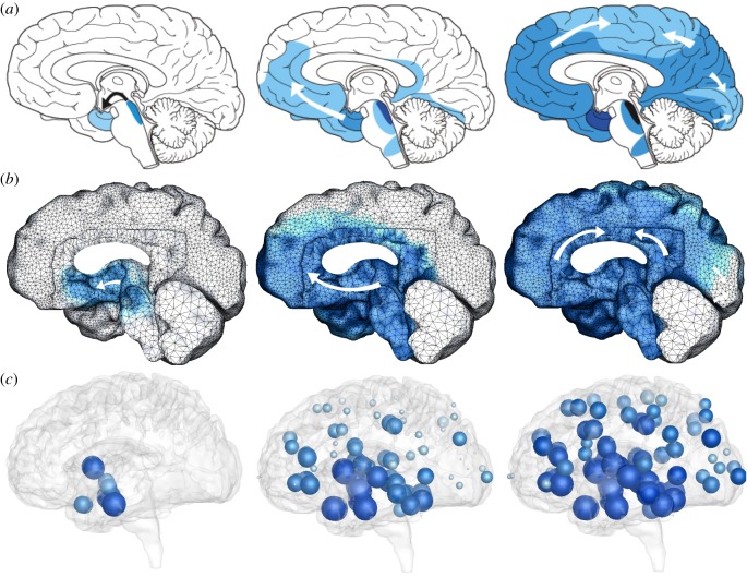
The current prevalent theory for neurodegenerative diseases is based on the prion-like paradigm [7] in which neurodegeneration is caused by the systematic invasion and conformational autocatalytic conversion of misfolded proteins [8]. In Alzheimer’s disease, Amyloid beta and tau proteins are believed to act in a prion-like manner and misfold [9]. This misfolded form of the protein acts as a template on which healthy proteins misfold and grow into increasingly larger aggregates [10]. Amyloid beta is an extracellular protein that mainly spreads across the extracellular matrix [11], whereas tau is an intracellular protein that primarily propagates within the network of axonal pathways [12]. Here, we focus on tau, which spreads across the brain in a highly predictable pattern [13]: misfolded tau proteins occur first in the locus coeruleus and the transentorhinal layer from where they spread to the transentorhinal region and the proper entorhinal cortex and ultimately affect all interconnected neocortical brain regions [14]. Figure 1a illustrates the typical spatio-temporal pattern of misfolded tau protein in Alzheimer’s disease inferred from histopathological observations of hundreds of human brains [15].

Figure 1.

Typical pattern of tau protein misfolding in Alzheimer’s disease. (a) Clinical observation [15], (b) continuum model [16] and (c) network spreading model display characteristic pattern with misfolded tau occurring first in the locus coeruleus and transentorhinal layer from where they spread to the transentorhinal region and the proper entorhinal cortex and ultimately affect all interconnected neocortical brain regions. (Online version in colour.)

Understanding the progression of Alzheimer’s disease is a matter of understanding the physical processes of misfolding and transport. From a modelling perspective, three approaches have been proposed to simulate the physics of neurodegeneration: (i) kinetic growth and fragmentation models to study the local interaction of aggregates of different sizes using a set of ordinary differential equations [17]; (ii) network diffusion models to study the global prion-like spreading of misfolded proteins using graph theory [5]; and (iii) reaction–diffusion-based continuum models to study the spatio-temporal evolution of patheogenic proteins using partial differential equations [18].

Figure 1b shows that continuum models with nonlinear reaction and anisotropic diffusion can accurately predict the typical pattern of tau protein misfolding in Alzheimer’s disease [16]. This simulation used a Fisher–Kolmogorov model [19,20], discretized with 400 000 tetrahedral finite elements and 80 000 d.f. The continuum model displays an excellent agreement with clinical observations. However, it is computationally expensive and impractical to systematically explore a wide variety of disease and treatment scenarios. In addition, there is currently no technology to validate its predicted spreading patterns at a high enough resolution that would truly warrant a finite-element simulation with thousands of degrees of freedom. The objective of this study is therefore to create an efficient and robust simulation tool that captures the key characteristic features of pathogenic proteins in Alzheimer’s disease by combining kinetic growth and fragmentation with network diffusion through a connectivity-weighted graph from the Human Connectome Project. Figure 1c suggests that—even with three orders of magnitude fewer degrees of freedom than the continuum models–our dynamic network model accurately predicts the typical spatio-temporal pattern of tau protein misfolding.

2. Kinetic models

To study the kinetics of protein misfolding, we consider three popular models with different levels of complexity, the simple one-concentration Fisher–Kolmogorov model [19], the two-concentration Heterodimer model [21] and the n-concentration Smoluchowski model [22].

2.1. The Fisher–Kolmogorov model

The simplest model to characterize protein misfolding is the Fisher–Kolmogorov model [19,20]. Initially proposed to model the spreading of a favoured gene in population dynamics, the Fisher–Kolmogorov model is now widely used to describe travelling wave solutions in ecology, physiology, combustion, crystallization, plasma physics, phase transition and biology [23]. It is based on a simple nonlinear reaction–diffusion equation for a single unknown, the misfolded protein concentration c,

$$\frac{\mathrm{d}\hspace{0.17em}c}{\mathrm{d}\hspace{0.17em}t}=\mathrm{\nabla }\cdot (\mathit{D}\hspace{0.17em}\cdot \mathrm{\nabla }c)+\alpha \hspace{0.17em}c\hspace{0.17em}[1-c],$$ 2.1

where D is the diffusion tensor that characterizes global protein spreading and α characterizes the local conversion rate from the healthy to the misfolded state as illustrated in figure 2.

Figure 2.

Kinetics of the Fisher–Kolmogorov model. The Fisher–Kolmogorov model has a single unknown, the misfolded protein concentration c. The model converts healthy to misfolded protein at a rate α. For the smallest perturbation from the healthy state, c > 0, all proteins will convert from the healthy to the misfolded state, c = 1. (Online version in colour.)

The Fisher–Kolmogorov equation (2.1) has two steady-state solutions, an unstable steady state at c = 0 and a stable steady state at c = 1. This implies that once misfolded protein is present anywhere in the brain, c > 0, the concentration will always be repelled from the benign state, c = 0, and attracted to the misfolded state, c = 1. While the Fisher–Kolmogorov model is attractive because of its simplicity and its low computational cost, its parameter α is purely phenomenological, it provides no insight into the mechanisms of infection, and it cannot capture intermediate equilibrium states as, for example, a result of pharmocological treatment.

2.2. The Heterodimer model

The simplest possible kinetic model that accounts for two configurations of the protein, the natural healthy state p and the misfolded state $\widetilde{\hspace{0.17em}p}$, is the Heterodimer model [21]. In this model, misfolded proteins recruit healthy proteins at a rate k_11′, healthy proteins bind to misfolded proteins and adopt their conformation at a rate k_1′2′, and the resulting polymer fragments into infectious seeds at a rate k_2′2,

$$p+\tilde{p}\stackrel{k_{{11}^{\prime }}}{\to }p\hspace{0.17em}\tilde{p}p\hspace{0.17em}\tilde{p}\stackrel{k_{1^{\prime }{2}^{\prime }}}{\to }\tilde{p}\hspace{0.17em}\tilde{p}\tilde{p}\hspace{0.17em}\tilde{p}\stackrel{k_{2^{\prime }2}}{\to }\tilde{p}+\tilde{p}.$$ 2.2

For simplicity, we collectively represent the conformational conversion from the healthy to the misfolded state as a single step through the rate constant k₁₂,

$$p+\tilde{p}\stackrel{k_{12}}{\to }\tilde{p}+\tilde{p}.$$ 2.3

These considerations motivate a system of governing equations for the spatio-temporal evolution of the total amount of healthy and misfolded proteins p and $\widetilde{\hspace{0.17em}p}$ [24],

$$\begin{array}{rl}\hfill \frac{\mathrm{d}p}{\mathrm{d}t}& =\mathrm{\nabla }\cdot (\mathit{D}\hspace{0.17em}\cdot \mathrm{\nabla }p)+k_0-k_1\hspace{0.17em}p-k_{12}\hspace{0.17em}p\hspace{0.17em}\tilde{p}\hfill \\ \mathrm{and}\frac{\mathrm{d}\hspace{0.17em}\tilde{p}}{\mathrm{d}\hspace{0.17em}t}\hfill & =\mathrm{\nabla }\cdot (\mathit{D}\hspace{0.17em}\cdot \mathrm{\nabla }\tilde{p})-{\tilde{k}}_1\hspace{0.17em}\tilde{p}+k_{12}\hspace{0.17em}p\hspace{0.17em}\tilde{p},\hfill \end{array}\}$$ 2.4

where D is the diffusion tensor that characterizes protein spreading, k₀ is the production rate of healthy protein, k₁ and ${\tilde{k}}_1$ are the clearance rates of healthy and misfolded proteins, and k₁₂ is the conversion rate from the healthy to the misfolded state, as illustrated in figure 3.

Figure 3.

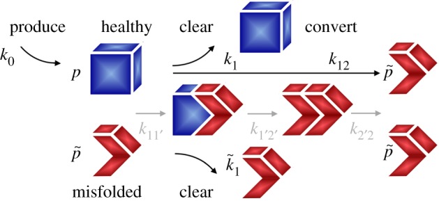
Kinetics of the Heterodimer model. The Heterodimer model has two unknowns, the healthy concentration p and the misfolded concentration $\tilde{p}$. The model produces healthy protein at a rate k₀, clears healthy and misfolded protein at rates k₁ and ${\tilde{k}}_1$, and converts healthy to misfolded protein at a rate k₁₂, which collectively represents the processes of recruitment k_11′, misfolding k_1′2′ and fragmentation k_2′2. (Online version in colour.)

In the initial healthy state, the healthy and misfolded protein concentrations are p₀ = k₀/k₁ and ${\tilde{p}}_0=0$; in the diseased state, they converge towards $p_{\mathrm{\infty }}={\tilde{k}}_1/k_{12}$ and ${\tilde{p}}_{\mathrm{\infty }}=k_0/{\tilde{k}}_1-k_1/k_{12}$.

We can simplify the Heterodimer model (2.4) by assuming that, initially, the amount of healthy protein is much larger than the amount of misfolded protein, $p\gg \tilde{p}$, which implies that dp/dt ≈ 0 and $\mathrm{\nabla }\cdot (\mathit{D}\hspace{0.17em}\cdot \mathrm{\nabla }p)\approx 0$. With these assumptions, equation (2.4) provides an explicit estimate of the amount of healthy protein p,

$$k_0-k_1\hspace{0.17em}p-k_{12}\hspace{0.17em}p\hspace{0.17em}\tilde{p}=0\text{thus}\hspace{0.17em}p=\frac{k_0}{k_1+k_{12}\hspace{0.17em}\tilde{p}}.$$ 2.5

We approximate the healthy protein concentration p using a Taylor series, $p=k_0/k_1\hspace{0.17em}[1-\tilde{p}\hspace{0.17em}{k}_{12}/k_1]$, and substitute this expression into equation (2.4),

$$\frac{\mathrm{d}\hspace{0.17em}\tilde{p}}{\mathrm{d}\hspace{0.17em}t}=\mathrm{\nabla }\cdot (\mathit{D}\hspace{0.17em}\cdot \mathrm{\nabla }\tilde{p})+[k_{12}\frac{k_0}{k_1}-{\tilde{k}}_1]\hspace{0.17em}\tilde{p}-\frac{k_{12}^2\hspace{0.17em}{k}_0}{k_1^2}\hspace{0.17em}{\tilde{p}}^2.$$ 2.6

By re-parametrizing equation (2.6) in terms of the misfolded protein concentration, $c=\tilde{p}/{\tilde{p}}^{\max }$ with ${\tilde{p}}^{\max }=k_1/k_{12}-k_1^2/k_{12}^2\hspace{0.17em}{\tilde{k}}_1/k_0$, we recover the special case of the Fisher–Kolmogorov model (2.1) for a single unknown, the misfolded protein concentration c,

$$\frac{\mathrm{d}\hspace{0.17em}c}{\mathrm{d}\hspace{0.17em}t}=\mathrm{\nabla }\cdot (\mathit{D}\hspace{0.17em}\cdot \mathrm{\nabla }c)+\alpha \hspace{0.17em}c\hspace{0.17em}[1-c]\text{with}\hspace{0.17em}\alpha =k_{12}\hspace{0.17em}\frac{k_0}{k_1}-{\tilde{k}}_1.$$ 2.7

Interestingly, the Fisher–Kolmogorov parameter α now takes a physical interpretation in terms of the rates of production k₀, clearance k₁ and ${\tilde{k}}_1$, and conversion k₁₂. While the Heterodimer model (2.4) strikes a natural balance between computational efficiency and mechanistic insight, it does not explicitly capture the size distribution of misfolded protein aggregates, their nucleation and fragmentation, and the response of the system to specific size-targeting antibodies.

2.3. The Smoluchowski model

To characterize the size distribution of misfolded protein aggregates, we consider the Smoluchowski model, a set of population balance equations that explicitly account for the kinetics of nucleation, aggregation, fragmentation and clearance of particles of different sizes [22]. For more than a century, the Smoluchowski model has been widely used in statistical physics to characterize processes of polymerization, coalescence of aerosols, emulsication and flocculation. It follows the n concentrations c_i of particles of size i = 1, …, n and explicitly models their aggregation and fragmentation through the individual aggregation and fragmentation rates a_ij and f_ij with i, j = 1, …, n,

$$c_i+c_{\hspace{0.17em}j}{\to }^{a_{ij}}\hspace{0.17em}{c}_{i+j}\text{and}{c}_{i+j}\stackrel{\hspace{0.17em}{f}_{ij}}{\to }{c}_i+c_{\hspace{0.17em}j}.$$ 2.8

We can summarize the collective effects of aggregation and fragmentation on the concentration c_i through the aggregation and fragmentation A_i and F_i,

$$\begin{array}{cc}\hspace{0.17em}& A_i=\sum _{\hspace{0.17em}j=1}^{i-1}{a}_{\hspace{0.17em}j(i-j)}{c}_{\hspace{0.17em}j}{c}_{i-j}-\sum _{\hspace{0.17em}j=1}^{\mathrm{\infty }}2a_{ij}{c}_i{c}_{\hspace{0.17em}j}\hfill \\ \mathrm{and}\hfill & F_i=\sum _{\hspace{0.17em}j=1}^{i-1}{f}_{\hspace{0.17em}j(i-j)}{c}_i-\sum _{\hspace{0.17em}j=1}^{\mathrm{\infty }}2f_{ij}{c}_{i+j}.\hfill \end{array}\}$$ 2.9

Aggregation of two smaller particles c_j and c_i−j creates new particles c_i and removes particles c_i as they aggregate with c_j to larger particles c_i+j. Fragmentation removes particles c_i as they fragment into two smaller particles c_j and c_j−i and adds new particles c_i from the fragmentation of larger particles c_i+j into c_i and c_j. Taken together, the Smoluchowski model tracks the size distribution of particles through a nonlinear system of reaction–diffusion equations for the unknown concentrations c_i [25],

$$\frac{\mathrm{d}\hspace{0.17em}{c}_i}{\mathrm{d}\hspace{0.17em}t}=\mathrm{\nabla }\cdot (\mathit{D}{\hspace{0.17em}}_i\cdot \mathrm{\nabla }{c}_i)+k_{0i}-k_i\hspace{0.17em}{c}_i+A_i-F_i,$$ 2.10

where D_i is the size-specific diffusion tensor, k₀ is the production rate, k_i is the clearance rate, and A_i and F_i are the size-specific aggregation and clearance rates according to aggregation–fragmentation kinetics (2.9). Here, we adopt a simplification of the Smoluchowski model (2.10), the nucleated polymerization model [26,27] with a nucleus size of two and spontaneous nucleation, to model the nucleation, aggregation, and fragmentation of tau proteins in Alzheimer’s disease [17] and make the following simplifying assumptions: we assume that diffusion is size-independent, D_i = D; production is only possible for healthy monomers, k₀₁ = k₀ for i = 1, but not for misfolded particles of any other size, k_0i = 0 for i > 1; clearance occurs at k₁ for healthy monomers, is size-independent k₂ = k_i for larger particles 1 < i < n; and impossible k_n = 0 for the largest particle size i = n; nucleation of two monomers occurs at a nucleation rate a₁₁ = κ and is irreversible; aggregation of larger particles is size-independent a_ij = a, but can only occur by adding single monomers for i = 1 or j = 1 and is impossible a_ij = 0 otherwise; fragmentation into monomers is impossible f_ij = 0 for i = 1 or j = 1, fragmentation into larger particles is size-independent f_ij = f for 1 < i, j < n, and fragmentation is impossible f_ij = 0 for the largest particle size i, j = n. This results in the following explicit set of equations for the concentrations of sizes 1, 2, i = 3, …, n − 1, and n [28],

$$\begin{array}{ccc}\hspace{0.17em}\hfill & \frac{\mathrm{d}{c}_1}{\mathrm{d}t}=\hfill & \mathrm{div}(\mathit{D}\cdot \mathrm{\nabla }{c}_1)+k_0-k_1{c}_1-2\kappa c_1^2-a{c}_1\sum _{j=2}^{n-1}{c}_j\hfill \\ \hspace{0.17em}\hfill & \frac{\mathrm{d}{c}_2}{\mathrm{d}t}=\hfill & \mathrm{div}(\mathit{D}\cdot \mathrm{\nabla }{c}_2)-k_2{c}_2+\kappa c_1^2-a{c}_1{c}_2+2f\sum _{j=2}^{n-3}\hspace{0.17em}{c}_{2+j}\hfill \\ \hspace{0.17em}\hfill & \frac{\mathrm{d}{c}_i}{\mathrm{d}t}=\hfill & \mathrm{div}(\mathit{D}\cdot \mathrm{\nabla }{c}_i)-k_i\hspace{0.17em}{c}_i-a{c}_1{c}_i+a{c}_1{c}_{i-1}+2f\sum _{j=2}^{n-i-1}{c}_{i+j}-f[i-3]c_i\hfill \\ \mathrm{and}\hfill & \frac{\mathrm{d}{c}_n}{\mathrm{d}t}=\hfill & \mathrm{div}(\mathit{D}\cdot \mathrm{\nabla }{c}_n)+a{c}_1{c}_{n-1}.\hfill \end{array}\}$$ 2.11

Figure 4 illustrates the Smoluchowski model for tau proteins. In addition to the global diffusion D, this model has six local kinetic parameters, the production of healthy monomers k₀, the clearance of healthy monomers k₁ and misfolded polymers k₂ = k_i, the nucleation κ, the aggregation a and the fragmentation f. Notably, the Smoluchowski model features two distinct mechanisms to convert healthy proteins into misfolded proteins [17]: primary conversion reflected through the nucleation rate κ and secondary conversion reflected through the aggregation rate a. While the Smoluchowski model follows the size distribution of individual aggregates, allows for size-specific transport, aggregation, fragmentation and clearance, and provides a mechanistic interpretation of the protein misfolding [29], its intrinsic disadvantage is its large number of parameters and, with it, the risk of overfitting.

Figure 4.

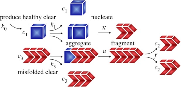
Kinetics of the Smoluchowski model. The Smoluchowski model has n unknowns c_i, one for the concentration of each size i = 1, …, n, where c₁ represents the concentration of healthy monomers. The model produces healthy protein at a rate k₀, clears healthy and misfolded protein at rates k₁ and k_i, nucleates two misfolded proteins from two healthy proteins at a rate κ, aggregates by adding single healthy proteins to misfolded filaments at a rate a, and fragments misfolded filaments at a rate f. (Online version in colour.)

3. Brain network models

A defining feature of prion-like diseases is the spreading of misfolded proteins from a small infected region along axonal fibre tracts throughout the entire brain [30]. We model this spreading as the diffusion across the brain’s connectome [31], which we represent as a weighted undirected graph $\mathcal{G}$ with N nodes and E edges.

3.1. The connectivity-weighted graph

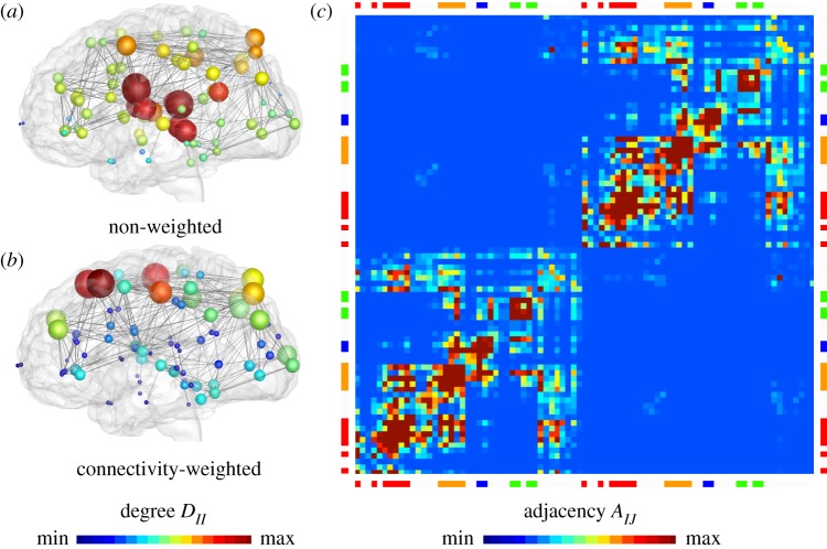
We extract the graph $\mathcal{G}$ from the tractography of diffusion tensor magnetic resonance images of 418 healthy subjects of the Human Connectome Project [32] using the Budapest Reference Connectome v. 3.0 [33]. While our method is generally applicable to graphs of any resolution, for illustrative purposes, we map the original graph with N = 1015 nodes and E = 37 477 edges onto a graph with N = 83 nodes and E = 1130 edges. This resolution corresponds to the widely used Freesurfer parcellation [34] and allows us to rapidly map the node representation back onto the brain surface. The degree of our initial graph, the number of edges per node, varies between 6 and 48, with fewest edges at the frontal pole and most edges at the caudate. We weight each edge by the mean fibre number n_IJ divided by the mean fibre length l_IJ averaged over all 418 brains. The mean fibre number varies between 1 ≤ n_IJ ≤ 596, with an average of ${\overline{n}}_{IJ}=40.2$ fibres per edge and most fibres between the superior parietal and the precuneus regions. The mean fibre length varies between 11.3 mm ≤ l_IJ ≤ 136.8 mm, with an average of ${\overline{l}}_{IJ}=38.40\hspace{0.17em}\text{mm}$ and the longest fibres between the lateral orbitofronal and the precuneus regions. Figure 5 illustrates our graph $\mathcal{G}$ with the edges colour-coded by the mean fibre number n_IJ, mapped onto a three-dimensional brain model from magnetic resonance images [35].

Figure 5.

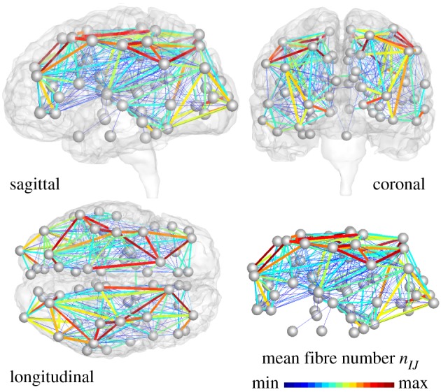
Brain network model. Misfolded tau proteins spread across the brain’s connectome represented as a weighted graph $\mathcal{G}$ with N = 83 nodes and E = 1130 edges. Edges are weighted by the mean fibre number n_IJ divided by the mean fibre length l_IJ averaged over 418 healthy brains from the Human Connectome Project. (Online version in colour.)

3.2. The graph Laplacian

We summarize the connectivity of the graph $\mathcal{G}$ in terms of the degree matrix D_II, a diagonal matrix that characterizes the degree of each node I, and the weighted adjacency matrix A_IJ, the ratio of mean fibre number and length between nodes I and J. The difference between the degree matrix D_IJ and the adjacency matrix A_IJ defines the weighted graph Laplacian L_IJ,

$$\begin{array}{rl}\hfill L_{IJ}& =D_{IJ}-A_{IJ}\hspace{0.17em}\mathrm{with}\hspace{0.17em}{A}_{IJ}=\frac{n_{IJ}}{l_{IJ}}\hfill \\ \mathrm{and}{D}_{II}\hfill & =\mathrm{diag}\sum _{J=1,J\ne I}^N{A}_{IJ}.\hfill \end{array}\}$$ 3.1

Figure 6a illustrates the degree D_II of the baseline non-weighted graph, and the degree D_II of our connectivity-weighted graph $\mathcal{G}$ (figure 6b) along with its adjacency A_IJ (figure 6c). For our connectivity-weighted graph, the degree varies between 2.1 ≤ D_II ≤ 127.6, with an average degree of ${\overline{D}}_{II}=42.8$ per node, and the lowest and highest degrees in the frontal pole, shown in blue, and in the precentral gyrus, shown in red. The adjacency matrix clearly reflects the small-world architecture of our brain with strongly connected hubs within the right and left hemispheres, indicated through the lower left and upper right quadrants, and strong connections within the four lobes, indicated through the eight red regions along the diagonal. The adjacency varies between 0.01 ≤ A_IJ ≤ 35.32, with an average adjacency of ${\overline{A}}_{IJ}=1.57$ per edge, and lowest and highest values between the superior parietal and the precuneus regions and between the lateral orbitofrontal and the isthmus cingulate regions. These pronounced variations in degree and adjacency confirm the general notion that the architecture of our brain resembles a small-world network [1] in which highly connected nodes are more likely to become infected and turn into hubs of misfolded protein spreading.

Figure 6.

Brain network model. The connectivity of the graph $\mathcal{G}$ is represented through the degree D_II, the number of edges per node, and the adjacency A_IJ = n_IJ/l_IJ, the ratio of fibre number and length. (a) Degree D_II of non-weighted and (b) connectivity-weighted graphs and (c) adjacency A_IJ of connectivity-weighted graph, averaged over 418 healthy brains from the Human Connectome Project. (Online version in colour.)

3.3. The network model

We assume that the weighted Laplacian L_IJ characterizes the spreading of healthy and misfolded proteins across the brain network and discretize our three kinetic models on our weighted undirected graph $\mathcal{G}$. Specifically, we introduce the concentrations c_I, p_I, ${\tilde{p}}_I$ and c_iI as global unknowns at the I = 1, …, N nodes of our graph $\mathcal{G}$. This results in the discretized sets of equations for the single concentration Fisher–Kolmogorov model (2.1) with N unknowns,

$$\frac{\mathrm{d}{c}_I}{\mathrm{d}t}=-\hspace{0.17em}\sum _{J=1}^N{L}_{IJ}{c}_J+\alpha c_I[1-c_I],\hspace{0.17em}$$ 3.2

for two-concentration Heterodimer model (2.4) with 2 N unknowns,

$$\begin{array}{ccc}\hspace{0.17em}\hfill & \frac{\mathrm{d}\hspace{0.17em}{p}_I}{\mathrm{d}t}=\hfill & -\sum _{J=1}^N{L}_{IJ}\hspace{0.17em}{p}_J+k_0-k_1{p}_I-k_{12}{p}_I\hspace{0.17em}{\tilde{p}}_I\hfill \\ \mathrm{and}\hfill & \frac{\mathrm{d}{\tilde{p}}_I}{\mathrm{d}t}=\hfill & -\sum _{j=1}^N{L}_{IJ}{\tilde{p}}_J-{\tilde{k}}_1{\tilde{p}}_I+k_{12}\hspace{0.17em}{p}_I{\tilde{p}}_I\hfill \end{array}\}$$ 3.3

and for the n-concentration Smoluchowski model (2.10) with n × N unknowns,

$$\frac{\mathrm{d}{c}_{iI}}{\mathrm{d}t}=-\hspace{0.17em}\sum _{J=1}^N{L}_{IJ}{c}_{iJ}+k_{0i}-k_i{c}_{iI}+A_{iI}-F_{iI}.$$ 3.4

We discretize our network models in time using either implicit or explicit time integration schemes to simulate the spatio-temporal evolution of misfolded proteins across the brain.

4. Biomarker models

A biomarker is a global metric to characterize the evolution of neurodegeneration across the brain [36]. We calculate the biomarker abnormality as the temporal evolution of the total concentration of misfolded proteins integrated across a specific region of interest or across the brain as a whole. Biomarker abnormalities of the individual lobes provide insight into the spatio-temporal sequence of infection; global biomarker abnormalities of the brain as a whole provide a window into the progression of neurodegeneration and the time line of infection.

4.1. The Fisher–Kolmogorov model

Figure 7 summarizes the biomarker abnormality in all four lobes throughout a time period of three decades as predicted by the Fisher–Kolmogorov model (3.2). For the simulation, we chose a conversion rate constant of α = 0.5 and seeded misfolded proteins by increasing the initial concentration in the entorhinal cortex to c₀ = 0.1. Our simulation uses an implicit time integration scheme with 100 times steps of Δt = 0.4 years, and runs 0.55 and 0.64 s without and with output on a standard laptop computer. Figure 1c summarizes the resulting activation sequence. We post-process the simulation to calculate the biomarker abnormality,

$$C(t)=\hspace{0.17em}\sum _{I=1}^N{c}_I(t).$$ 4.1

as the discrete sum of the misfolded protein concentration c_I at the I nodes of the temporal, frontal, parietal and occipital lobes, and of the brain as a whole. All biomarker curves in figure 7 display a smooth sigmoidal form, which is in excellent agreement with brain network spreading models in general [37] and with clinical biomarker models of neurodegeneration in particular [36]. The individual biomarkers of the four lobes reveal the characteristic spreading of misfolded tau protein in Alzheimer’s disease starting in the temporal lobe, shown in green, followed by the frontal, parietal, and occipital lobes, shown in red, orange, and blue. This activation sequence agrees well with the clinically observed spreading pattern [14] in figure 1a. For comparison, the dashed grey and black lines in figure 7 show the biomarker integrated over the entire brain as predicted by the continuum model [16] in figure 1b and by the Fisher–Kolmogorov network model in figure 1c. This quantitative comparison confirms that, even at a much lower spatial resolution, our network model captures the integral characteristics of continuum models for Alzheimer’s disesase [38].

Figure 7.

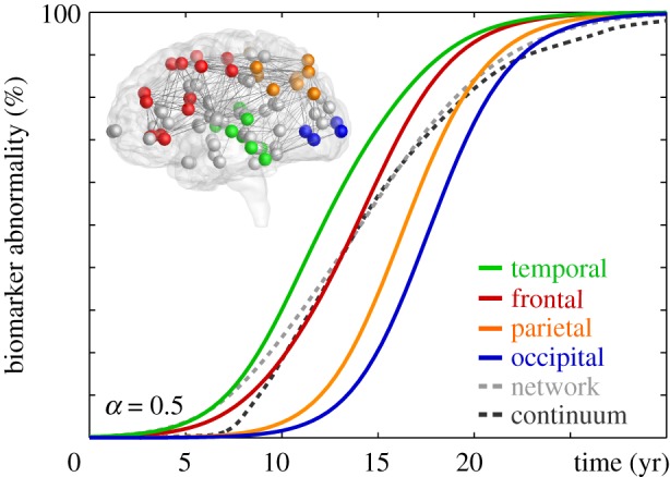
Biomarker abnormality of Fisher–Kolmogorov model. Integrating the concentration of misfolded proteins c across individual lobes reveals the characteristic activation sequence in Alzheimer’s disease from the temporal lobe to the frontal, parietal and occipital lobes. The dashed grey and black lines highlight the biomarker abnormality $\mathcal{C}$ of the Fisher–Kolmogorov network and continuum model in figure 1 integrated across the entire brain. (Online version in colour.)

4.2. The Heterodimer model

Figure 8 summarizes the biomarker abnormality in all four lobes, similar to figure 7, but now, instead of using the one-concentration Fisher–Kolmogorov model (3.2), using the two-concentration Heterodimer model (3.3). For the simulation, we chose a production rate of k₀ = 1.0, clearance rates of k₁ = 0.5 and ${\tilde{k}}_1=0.5$, and a conversion rate of k₁₂ = 0.5, which results in an initial healthy concentration of p₀ = 2.0 and an initial misfolded concentration of ${\tilde{p}}_0=0.0$, which we increased locally in the entorhinal cortex to ${\tilde{p}}_0=0.1$ to seed misfolding. Our simulation uses an implicit time integration scheme with 100 times steps of Δt = 0.4 years, and runs slightly longer than the Fisher–Kolmogorov model, but still completes in 0.66 and 0.68 s without and with output on a standard laptop computer. Again we calculate the biomarker abnormality,

$$\tilde{P}(t)=\hspace{0.17em}\sum _{I=1}^N{\tilde{p}}_I(t).$$ 4.2

as the discrete sum of the misfolded protein concentration ${\tilde{p}}_I$ at the I nodes of the four lobes and of the brain as a whole. Figure 8 confirms that, for a conversion rate, $\alpha =k_{12}\hspace{0.17em}{k}_0/k_1-{\tilde{k}}_1$ in accordance with equation (2.7), the Heterodimer model predicts an identical infection sequence and similar biomarker curves as the Fisher–Kolmogorov model: The green, red, orange and blue curves of the individual lobes and the dashed grey curve of the whole brain in figure 8 are indistinguishable from the curves in figure 7. This suggests that, if we are exclusively interested in the spreading of misfolded protein, from an initial healthy to a fully misfolded state, we can use the simple Fisher–Kolmogorov model (3.2) without loss of accuracy and interpret its phenomenological rate constant α as a combination of the mechanistic rate constants k₀, k₁, ${\tilde{k}}_1$ and k₁₂ of the Heterodimer model.

Figure 8.

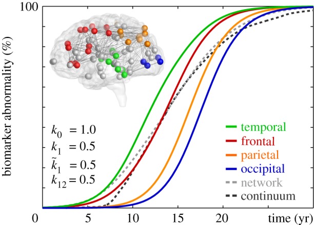
Biomarker abnormality of Heterodimer model. Integrating the concentration of misfolded proteins $\tilde{p}$ across individual lobes reveals the characteristic activation sequence in Alzheimer’s disease from the temporal lobe to the frontal, parietal and occipital lobes. The dashed grey and black lines highlight the biomarker abnormality $\tilde{\mathcal{P}}$ of the Heterodimer network and continuum model in figure 1 integrated across the entire brain. (Online version in colour.)

4.3. Infection times

We now adopt the Heterodimer model to study the regional vulnerability of different brain regions. Specifically, we successively seed misfolded protein in all N = 83 regions, simulate the spatio-temporal spreading across the brain, calculate the resulting 83 biomarker curves, and quantify the individual infection times. Figure 9 summarizes the biomarker curves and their associated brain regions colour-coded by infection time. Misfolded proteins spread fastest when seeded in the putamen or insula with a total infection times of 20.2 years, shown in red, and slowest when seeded in the frontal pole and entorhinal region with infection times of 30.4 and 28.8 years, shown in blue. The significant variation in infection times, by more than 10 years, underlines the heterogeneity of the brain network with a few highly connected hubs [1]. These observations agree well with the hierarchical spread of epidemic outbreaks known from general network theory [39]. For comparison, the dashed grey line illustrates the lower limit of the infection time of 16.6 years, associated with a homogeneous seeding across all N = 83 regions. The mean infection time of 24.9 years on the heterogeneous network is almost exactly 50% longer. Interestingly, the entorhinal cortex, which is known as the region where misfolded tau proteins are first observed [14], is associated with the second longest in infection time. This could explain, at least in part, why tau pathology is so difficult to detect during the early stages of Alzeimer’s disease [13]. The heterogeneous vulnerability of the brain network in figure 9 presents opportunities when designing treatment strategies: Reducing the local accumulation of misfolded protein in highly infectious regions such as the putamen or the insula will have a more pronounced effect on slowing down neurodegeneration than intervening in poorly connected regions such as the frontal pole. The following section focusses on different potential treatment options.

Figure 9.

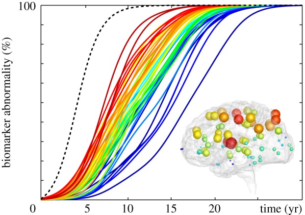
Infection times. Biomarker curves for misfolded protein seeding in N = 83 seeding regions illustrate the regional vulnerability of the network model. Misfolded proteins spread fastest when seeded in the putamen or insula, red spheres and curves, and slowest when seeded in the frontal pole and entorhinal region, blue spheres and curves. The dashed grey line highlights the lower limit of the infection time associated with a homogeneous seeding across all regions. (Online version in colour.)

5. Treatment opportunities

Now that we have established a solid baseline simulation for the progression of Alzheimer’s disease that agrees well with clinical observations, we explore the potential of our models for simulating different treat opportunities. Two promising therapeutic strategies are currently emerging to delay or even prevent the progression of Alzheimer’s disease [40]: reducing misfolding [41] and increasing clearance [42]. Even if, to date, we do not have a precise knowledge about all the model parameters, we can still perform numerical experiments to elaborate the mechanisms and time scales associated with these interventions.

5.1. Delaying conversion

Figures 10 and 11 reveal the effects of reducing misfolding and increasing clearance with the Fisher–Kolmogorov model. The only model parameter is the conversion rate $\alpha =k_{12}\hspace{0.17em}{k}_0/k_1-{\tilde{k}}_1$, which we can interpret as a combination of production k₀, clearance k₁ and ${\tilde{k}}_1$, and conversion k₁₂. Figures 10 and 11 illustrate simulations of the baseline case with α = 0.5, and reduced values of α, which collectively mimic reduced misfolding k₁₂ and increased clearance ${\tilde{k}}_1$. The simulations confirm our intuition that decreasing the conversion α delays the accumulation of the misfolded protein c and with it the biomarker abnormality $\mathcal{C}$. However, figures 10 and 11 also illustrate an inherent limitation of the Fisher–Kolmogorov model: once misfolded protein is present anywhere in the brain, the concentration will always be repelled from the healthy state and attracted to the misfolded state. While the Fisher–Kolmogorov model (2.1) is a simple model to efficiently explore the dynamics of protein misfolding on more complex three-dimensional finite-element geometries [16] and to study the interplay of biochemical and biomechanical degeneration [38], for applications with intermediate states, we recommend using more mechanistic kinetic models like the Heterodimer model (2.4) or the Smoluchowski model (2.10).

Figure 10.

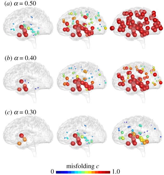
Delaying conversion. The Fisher–Kolmogorov model predicts that lower conversion rates α delay the increase of misfolded protein c. Baseline Alzheimer’s disease (a) and Alzheimer’s disease with moderately (b) and markedly (c) reduced conversion α from the healthy to the misfolded state. (Online version in colour.)

Figure 11.

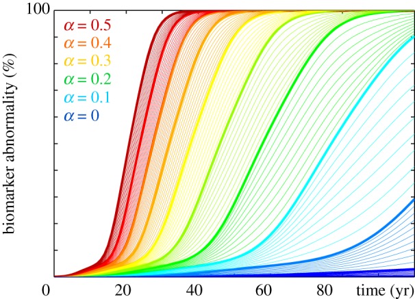
Reducing biomarker abnormality through delayed conversion. Decreasing the conversion α delays the accumulation of the misfolded protein concentration c and with it the biomarker abnormality $\mathcal{C}$. Irrespective of the conversion rate α, the misfolded protein concentration of the Fisher–Kolmogorov model always converges towards the fully misfolded state with a biomarker abnormality of $\mathcal{C}=100\text{\%}$. (Online version in colour.)

5.2. Reducing misfolding

Figures 12 and 13 illustrate the effect of reducing misfolding with the Heterodimer model. A turnover rate of k₁₂ = 0.50 predicts the baseline progression of Alzheimer’s disease in agreement with figure 1. For this baseline case with a production of k₀ = 1.0, clearances of k₁ = 0.5 and ${\tilde{k}}_1=0.5$, and a conversion of k₁₂ = 0.5 the Heterodimer model is identical to the Fisher–Kolmogorov model with a conversion of α = 0.50. According to equation (2.7), decreasing the Heterodimer conversion to k₁₂ = 0.40 would correspond to decreasing the Fisher–Kolmogorov conversion to α = 0.3. However, the k₁₂ = 0.40 pattern in figure 12 and the α = 0.3 pattern in figure 10 show significant differences: decreasing the turnover rate moderately to k₁₂ = 0.45 and markedly to k₁₂ = 0.40 not only delays but also reduces the accumulation of misfolded protein $\tilde{p}$ and with it the biomarker abnormality $\tilde{\mathcal{P}}$. Strikingly, in the early stages of neurodegeneration, even a small reduction of misfolding can delay disease progression by several decades [41] and reduce the resting state of misfolded protein ${\tilde{p}}_{\mathrm{\infty }}=k_0/{\tilde{k}}_1-k_1/k_{12}$ below its untreated value, here to ${\tilde{p}}_{\mathrm{\infty }}=0.89$ for k₁₂ = 0.45 and to ${\tilde{p}}_{\mathrm{\infty }}=0.75$ for k₁₂ = 0.40.

Figure 12.

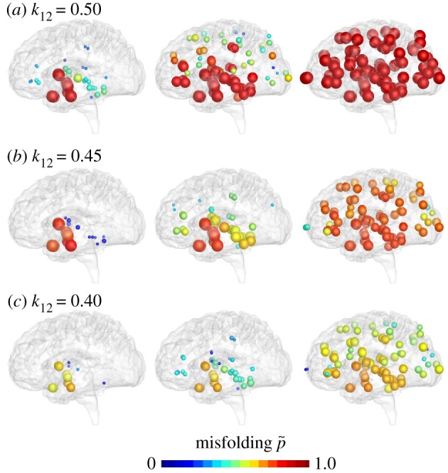
Reducing misfolding. The Heterodimer model predicts that lower turnover rates k₁₂ delay and reduce the accumulation of misfolded protein $\tilde{p}$. Baseline Alzheimer’s disease (a) and Alzheimer’s disease with moderately (b) and markedly (c) reduced turnover k₁₂ from the healthy to the misfolded state. (Online version in colour.)

Figure 13.

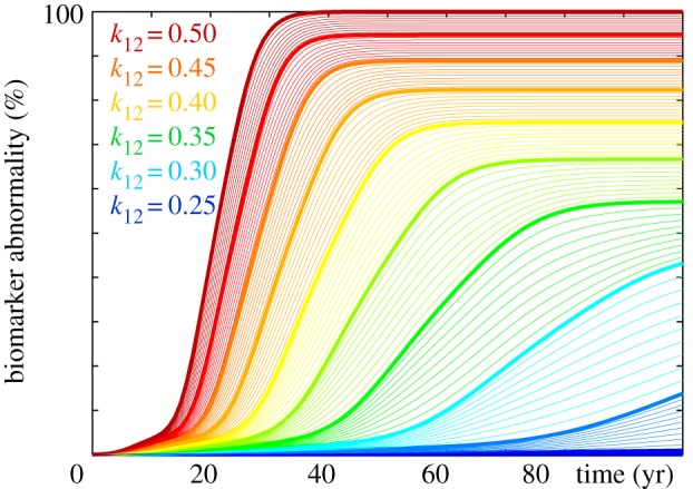
Reducing biomarker abnormality through reduced misfolding. Decreasing the turnover k₁₂ delays and reduces the accumulation of misfolded tau protein $\tilde{p}$ and with it the biomarker abnormality $\tilde{\mathcal{P}}$. Depending on the turnover rate k₁₂, the misfolded protein concentration of the Heterodimer model can converge towards intermediate states with a reduced biomarker abnormality of $\tilde{\mathcal{P}}<100\text{\%}$. (Online version in colour.)

5.3. Increasing clearance

Figures 14 and 15 highlight the effect of increasing clearance with the Heterodimer model. A clearance rate of ${\tilde{k}}_1=0.50$ predicts the baseline progression of Alzheimer’s in agreement with figure 1. For this baseline case, the Heterodimer model is identical to the Fisher–Kolmogorov model with a conversion of α = 0.50. According to equation (2.7), increasing the clearance to ${\tilde{k}}_1=0.70$ would correspond to decreasing the conversion to α = 0.3. But, similar to the previous example, the ${\tilde{k}}_1=0.70$ pattern in figure 14 and the α = 0.3 pattern in figure 10 show significant differences: increasing the clearance rate ${\tilde{k}}_1$ has similar effects as decreasing the turnover rate k₁₂; it not only delays but also reduces the accumulation of misfolded protein $\tilde{p}$ and with it the biomarker abnormality $\mathcal{P}$. Similar to a decreased turnover, an increased clearance can delay disease progression by several decades [42] and reduce the resting state of misfolded protein ${\tilde{p}}_{\mathrm{\infty }}=k_0/{\tilde{k}}_1-k_1/k_{12}$ significantly below its untreated value, here to ${\tilde{p}}_{\mathrm{\infty }}=0.67$ for ${\tilde{k}}_1=0.60$ and to ${\tilde{p}}_{\mathrm{\infty }}=0.43$ for ${\tilde{k}}_1=0.70$. While the Heterodimer model provides valuable insight into the clearance of all misfolded proteins, it cannot predict the effect of the selective clearance of small molecules.

Figure 14.

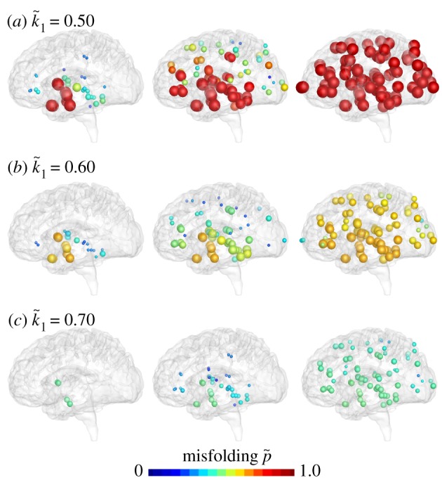
Increasing clearance. The Heterodimer model predicts that higher clearance rates ${\tilde{k}}_1$ delay and reduce the accumulation of misfolded protein $\tilde{p}$. Baseline Alzheimer’s disease (a) and Alzheimer’s disease with moderately (b) and markedly (c) increased clearance ${\tilde{k}}_1$ of misfolded protein. (Online version in colour.)

Figure 15.

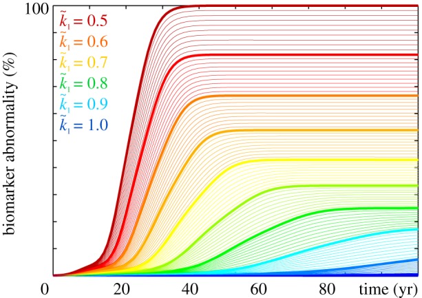
Reducing biomarker abnormality through increased clearance. Increasing the clearance ${\tilde{k}}_1$ delays and reduces the accumulation of misfolded tau protein $\tilde{p}$ and with it the biomarker abnormality $\tilde{\mathcal{P}}$. Depending on the clearance rate ${\tilde{k}}_1$, the misfolded protein concentration of the Heterodimer model can converge towards intermediate states with a reduced biomarker abnormality of $\tilde{\mathcal{P}}<100\text{\%}$. (Online version in colour.)

6. Size matters

In this last example, we explore the interplay of nucleation, aggregation, fragmentation and the general distribution of particle size using the Smoluchowski model and highlight its advantages over the Fisher–Kolmogorov and Heterodimer models.

6.1. Biomarker spectrum

To illustrate the dynamics of the Smoluchowski model, we consider the biomarker spectrum of the principal moments of the size distribution, the overall concentration of misfolded proteins c_i above a critical size i ≥ j,

$${\mathcal{C}}_{\hspace{0.17em}j}(t)=\sum _{I=1}^N\sum _{i=j}^n\hspace{0.17em}{c}_{iI}(t),$$ 6.1

and the overall mass of misfolded proteins i c_i above a critical size i ≥ j,

$${\mathcal{M}}_{\hspace{0.17em}j}(t)=\sum _{I=1}^N\sum _{i=j}^n\hspace{0.17em}i\hspace{0.17em}{c}_{iI}(t),$$ 6.2

where c_iI denotes the concentration of proteins of length i = 1, …, n at node I = 1, …, N. Specifically, ${\mathcal{C}}_2$ and ${\mathcal{M}}_2$ denote the total aggregate concentration and the total aggregate mass, and $\overline{c}={\mathcal{M}}_2/{\mathcal{C}}_2$ denotes the mean aggregate length. Figure 16 illustrates the biomarker spectrum ${\mathcal{M}}_{\hspace{0.17em}j}$ for a simulation with a production rate of k₀ = 1.0, clearance rates of k₁ = 0.5 for healthy monomers, k₂ = k_i = 0.5 for aggregates, and k_n = 0.0 for the particles of the largest size, an aggregation rate of a = 10.0, a fragmentation rate of f = 0.048, and nucleation rates of κ = 0.00016 in the entorhinal cortex and κ = 0.0 in all other regions. There is a large uncertainty about the true values for these rate constants and they may differ highly between variants [26]. Naturally, the choice of these rates will affect the sequence of events and the interplay of nucleation, aggregation, fragmentation and spread [28]. Here, we chose the parameter values such that their order of magnitude closely followed reported values in the literature [43], where the largest rate constant is the monomer production k₀ followed by the monomer clearance k₁, the polymer clearance k_i, the fragmentation f and the nucleation κ. Because of the small time constants, we now have to use a finer time discretization with 1000 times steps of Δt = 0.04 years, and we now use an explicit time integration. Our average simulation with n = 50 discrete aggregate sizes runs 1.97 and 2.20 s without and with output on a standard laptop computer; increasing the number of aggregates to n = 500 increases the simulation time to 6.96 and 16.43 seconds without and with output. Interestingly, the mass of all misfolded proteins ${\mathcal{M}}_2$, the dark red curve in figure 16, is almost indistinguishable from dashed black curve that highlights the biomarkers $\mathcal{C}$ of the Fisher–Kolmogorov model in figure 7 and $\tilde{\mathcal{P}}$ of the Heterodimer model in figure 8. However, in contrast to the Fisher–Kolmogorov and Heterodimer models, the Smoluchowski model features several competing mechanisms and time scales and allows for two distinct types of conversion, nucleation and aggregation. To better understand the dynamics of the Smoluchowski model, we explored the parameter space and learned that increasing the production k₀, the aggregation a, or the fragmentation f accelerates and increases protein misfolding and shifts the curves in figure 16 to the left and upward; increasing the nucleation κ accelerates protein misfolding and shifts the curves to the left, but not upward; and increasing the clearance k₁ or k₂ = k_i decelerates and reduces protein misfolding and shifts the curves to the right and downward. The initial time delay between the red ${\mathcal{M}}_2$ curve for c_i ≥ 2 and the blue ${\mathcal{M}}_{50}$ curve for c_i = 50 illustrates the aggregation dynamics, and confirms our intuition that smaller particles have to form first to trigger the aggregation of larger particles. Intermediate aggregate sizes, 20 ≤ c_i ≤ 30, highlighted through the yellow ${\mathcal{M}}_{20}$ to green ${\mathcal{M}}_{30}$ curves, display a small bump and increase initially, but then either partially clear or fragment into smaller aggregates.

Figure 16.

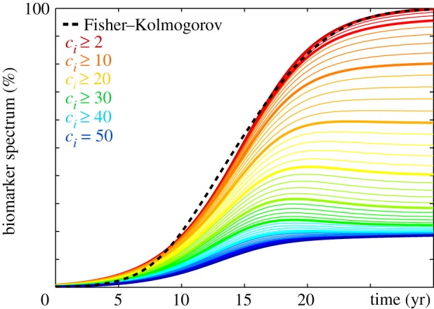
Biomarker spectrum of Smoluchowski model. Integrating the mass of misfolded proteins i c_i larger than a critical toxic size i reveals the characteristic nucleation, aggregation, fragmentation dynamics in Alzheimer’s disease. The red line ${\mathcal{M}}_2$ indicates the total mass of all misfolded proteins c_i ≥ 2; the blue line ${\mathcal{M}}_{50}$ indicates the mass of all aggregates of the largest size c_i = 50. The dashed black line highlights the biomarker abnormality $\mathcal{C}$ of the Fisher–Kolmogorov model in figure 7 and $\tilde{\mathcal{P}}$ of the two-concentration model in figure 8. (Online version in colour.)

6.2. Aggregate size distribution

Figure 17 illustrates the emerging aggregate size distribution and explains the dynamic features of the model: strikingly, the mean particle size, highlighted through the colour-coded dots, increases during the early stages of infection up to a mean particle size of 24.8 after 5.3 years, but then decreases gradually during the later stages towards a converged mean particle size of 15.7 after 30 years. This agrees well with the dynamics of the Smoluchowski model, which is known to predict an initial increase of the average particle size followed by a gradual decrease towards the homeostatic mean [43]. The red curve of the converged aggregate size distribution agrees well with the dashed black line of the analytical solution [43].

Figure 17.

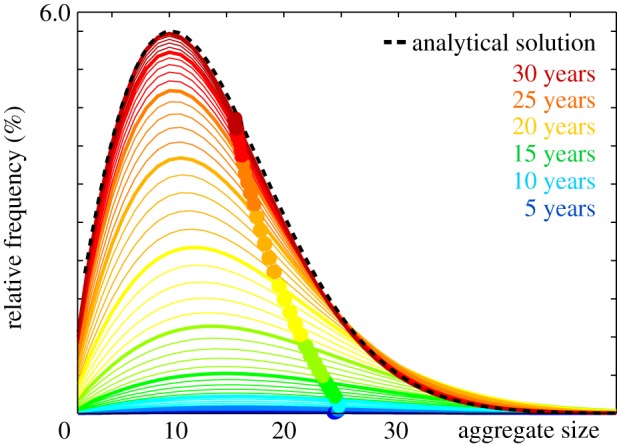
Emerging aggregate size distribution. During the early stages of infection, the mean aggregate size increases; during the later stages, it decreases gradually towards a homeostatic mean. Colour-coded lines indicate the evolution of aggregate size and frequency; dots show the evolution of the mean aggregate size; dashed black line highlights the analytical solution [43]. (Online version in colour.)

Figure 18 illustrates the spatio-temporal evolution of aggregates of different sizes. For illustrative purposes, rather then showing the discrete network with the individual N = 83 nodes, we colour-coded the associated 83 brain regions according to their misfolded protein concentration using the software tool Freesurfer [34]. The time lapse images show that misfolded tau proteins occur first in the locus coeruleus and transentorhinal layer from where they spread to the transentorhinal region and the proper entorhinal cortex and ultimately affect all interconnected neocortical brain regions. This spreading pattern agrees well with clinical observations [15], the continuum model of tau protein spreading [16], and our predictions with the Fisher–Kolmogorov and Heterodimer models in figure 1. Initially, the emerging aggregates are small, but they grow into progressively larger sizes as suggested by the biomarker spectrum in figure 16, and converge towards the final aggregate size distribution as indicated in figure 17. While analytical approximations exist to predict the biomarker curve and final size distribution for size-independent model parameters [43], numerical methods are necessary to predict the effect of selective parameter changes on these global readouts of the model.

Figure 18.

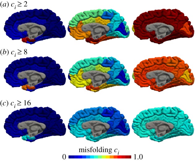
Typical pattern of tau aggregation in Alzheimer’s disease. The Smoluchowski model predicts that misfolded tau proteins occur first in the locus coeruleus and transentorhinal layer from where they spread to the transentorhinal region and the proper entorhinal cortex and ultimately affect all interconnected neocortical brain regions. Smaller aggregates emerge first (a) and grow progressively into moderate (b) and large (c) aggregates. (Online version in colour.)

6.3. Size-specific treatment

Figure 19 highlights the effect of selective size-targeted clearance on the biomarker spectrum as predicted by the numerical Smoluchowski model. A homogeneous clearance rate of k_i = 0.50 as indicated by the red biomarker spectrum, predicts the baseline progression of Alzheimer’s disease in agreement with figure 16. Increasing the clearance of a single specific aggregate size i from k_i = 0.5 to k_i = 10, while keeping all other clearance rates unchanged, delays and reduces the accumulation of misfolded tau protein c_i and with it the biomarker spectrum $\mathcal{M}$. Clearing a specific aggregate size i at a higher rate not only affects smaller aggregate sizes through a reduced fragmentation but also larger aggregate sizes through a reduced aggregation, which, collectively, results in an overall narrower biomarker spectrum. Increasing the target size of clearance, here from c₂ shown in orange to c₆ shown in blue decelerates and reduces protein misfolding and increases narrowing of the overall spectrum. Taken together, while the Fisher–Kolmogorov model and the Heterodimer model provide valuable insight into the kinetics of protein misfolding, only the Smoluchowski model can explain the interplay between primary conversion through nucleation, secondary conversion through aggregation, and the general distribution of particle size. Although targeting a single specific size might seem rather hypothetical, we can envision therapeutic approaches that target the production or clearance of small particles below a characteristic size [44].

Figure 19.

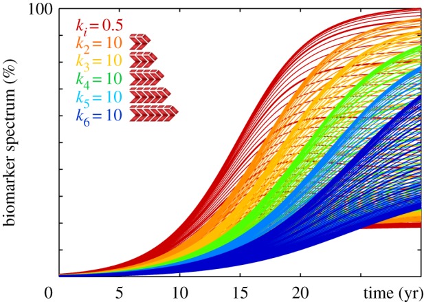
Reducing biomarker spectrum through size-targeted clearance. Increasing the clearance k_i of a single specific aggregate size delays and reduces the accumulation of misfolded tau protein c_i and with it the biomarker spectrum $\mathcal{M}$. Increasing the target size of clearance, here from c₂ to c₆ decelerates and reduces protein misfolding and narrows the overall size distribution. The red curves highlight the biomarker spectrum for the baseline model with a homogeneous clearance in figure 16. (Online version in colour.)

7. Conclusion

Despite their complexity, neurodegenerative diseases display remarkably consistent histopathological patterns. In Alzheimer’s disease, these invasion patterns are highly correlated with the spreading of misfolded amyloid beta and tau proteins. Here, we modelled the spreading of tau proteins by combining misfolding kinetics and network diffusion through a connectivity-weighted graph. In our dynamic brain network model, the concentrations of healthy and misfolded protein emerge dynamically at each node and propagate across the graph through its connectivity-weighted edges. Our model correctly predicts the spatio-temporal spreading pattern of tau in Alzheimer’s disease. There is currently no in vivo technology to quantify these spreading patterns longitudinally and non-invasively in humans. Our model provides a computational window into the interacting time scales and mechanisms of neurodegeneration. Its computational efficiency allows us to rapidly screen the landscape of disease-specific parameters that govern the kinetics of protein misfolding and spreading. We have demonstrated the potential of our model by simulating biomarker curves, aggregate size distributions, infection times and therapeutic intervention. A better understanding of the spreading of misfolded proteins could open new therapeutic opportunities towards blocking protein misfolding and promoting protein clearance using antibodies or small molecules. Ultimately, we envision that brain network models can help us answer some of the fundamental open questions in neurodegeneration: Why do neurodegenerative diseases progress so slowly, but yet so highly reproducibly? Can we identify early biomarkers of neurodegeneration that would allow us to interfere early? Why is neurodegeneration currently unstoppable? Can we interfere therapeutically and what would be the best time to do so? What are the roles of intra- and extracellular propagation? Can we manipulate spreading and where do we best interfere? What is the timeline of neurodegeneration? Can we predict personalized risk curves for individuals and estimate the socio-economic burden for an entire population? While we are still far from answering these questions, we believe that quantitative brain network modelling is a promising step towards identifying the key mechanisms of neurodegeneration and their roles in neurodegenerative disease.

Data accessibility

This article does not contain any additional data.

Competing interests

We declare we have no competing interests.

Funding

This work was supported by the Engineering and Physical Sciences Research Council grant no. EP/R020205/1 to A.G. and by the National Science Foundation grant no. CMMI 1727268 to E.K.

References

- 1.Bassett DS, Bullmore E. 2006. Small-world brain networks. Neuroscientist 12, 512–523. ( 10.1177/1073858406293182) [DOI] [PubMed] [Google Scholar]
- 2.Bassett DS, Bullmore ET. 2017. Small-world brain networks revisited. Neuroscientist 23, 499–516. ( 10.1177/1073858416667720) [DOI] [PMC free article] [PubMed] [Google Scholar]
- 3.Bullmore E, Sporns O. 2009. Complex brain networks: graph theoretical analysis of structural and functional systems. Nat. Rev. Neurosci. 10, 186–198. ( 10.1038/nrn2575) [DOI] [PubMed] [Google Scholar]
- 4.Kuhl E. 2019. Connectomics of neurodegeneration. Nat. Neurosci. 22, 1200–1202. ( 10.1038/s41593-019-0459-3) [DOI] [PubMed] [Google Scholar]
- 5.Raj A, Kuceyeski A, Weiner M. 2012. A network diffusion model of disease progression in dementia. Neuron 73, 1204–1215. ( 10.1016/j.neuron.2011.12.040) [DOI] [PMC free article] [PubMed] [Google Scholar]
- 6.Iturria-Medina Y, Sotero RC, Toussaint PJ, Evans AC, Initiative ADN. 2014. Epidemic spreading model to characterize misfolded proteins propagation in aging and associated neurodegenerative disorders. PLoS Comput. Biol. 10, e1003956 ( 10.1371/journal.pcbi.1003956) [DOI] [PMC free article] [PubMed] [Google Scholar]
- 7.Jucker M, Walker LC. 2011. Pathogenic protein seeding in Alzheimer disease and other neurodegenerative disorders. Ann. Neurol. 70, 532–540. ( 10.1002/ana.v70.4) [DOI] [PMC free article] [PubMed] [Google Scholar]
- 8.Prusiner SB. 1998. Prions. Proc. Natl Acad. Sci. USA 95, 13 363–13 383. ( 10.1073/pnas.95.23.13363) [DOI] [PMC free article] [PubMed] [Google Scholar]
- 9.Ittner LM, Gotz J. 2011. Amyloid-beta and tau – a toxic pas de deux in Alzheimer’s disease. Nat. Rev. Neurosci. 12, 67–72. ( 10.1038/nrn2967) [DOI] [PubMed] [Google Scholar]
- 10.Goedert M. 2015. Alzheimer’s and Parkinson’s diseases: the prion concept in relation to assembled Aβ, tau, and α-synuclein. Science 349, 1255555 ( 10.1126/science.1255555) [DOI] [PubMed] [Google Scholar]
- 11.Eisenberg D, Jucker M. 2012. The amyloid state of proteins in human diseases. Cell 148, 1188–1203. ( 10.1016/j.cell.2012.02.022) [DOI] [PMC free article] [PubMed] [Google Scholar]
- 12.Bressloff PC, Newby JM. 2013. Stochastic models of intracellular transport. Rev. Mod. Phys. 85, 135–196. ( 10.1103/RevModPhys.85.135) [DOI] [Google Scholar]
- 13.Walker LC, Jucker M. 2015. Neurodegenerative diseases: expanding the prion concept. Annu. Rev. Neurosci. 38, 87–103. ( 10.1146/annurev-neuro-071714-033828) [DOI] [PMC free article] [PubMed] [Google Scholar]
- 14.Braak H, Braak E. 1991. Neuropathological stageing of Alzheimer-related changes. Acta Neuropathol. 82, 239–259. ( 10.1007/BF00308809) [DOI] [PubMed] [Google Scholar]
- 15.Jucker M, Walker LC. 2013. Self-propagation of pathogenic protein aggregates in neurodegenerative diseases. Nature 501, 45–51. ( 10.1038/nature12481) [DOI] [PMC free article] [PubMed] [Google Scholar]
- 16.Weickenmeier J, Kuhl E, Goriely A. 2018. The multiphysics of prion-like diseases: progression and atrophy. Phys. Rev. Lett. 121, 158101 ( 10.1103/PhysRevLett.121.158101) [DOI] [PubMed] [Google Scholar]
- 17.Knowles TPJ, Waudby CA, Devlin GL, Cohen SIA, Aguzzi A, Vendruscolo M, Terentjev EM, Welland ME, Dobson CM. 2009. An analytical solution to the kinetics of breakable filament assembly. Science 326, 1533–1537. ( 10.1126/science.1178250) [DOI] [PubMed] [Google Scholar]
- 18.Weickenmeier J, Jucker M, Goriely A, Kuhl E. 2019. A physics-based model explains the prion-like features of neurodegeneration in Alzheimer’s disease, Parkinson’s disease, and amyotrophic lateral sclerosis. J. Mech. Phys. Solids 124, 264–281. ( 10.1016/j.jmps.2018.10.013) [DOI] [Google Scholar]
- 19.Fisher RA. 1937. The wave of advance of advantageous genes. Ann. Eugen. 7, 355–369. ( 10.1111/j.1469-1809.1937.tb02153.x) [DOI] [Google Scholar]
- 20.Kolmogorov AN. 1937. A study of the equation of diffusion with increase in the quantity of matter, and its application to a biological problem. Moscow Univ. Bull. Math. 1, 1–25. [Google Scholar]
- 21.Prusiner SB. et al. 1990. Transgenic studies implicate interactions between homologous PrP isoforms in scrapie prion replication. Cell 63, 673–686. ( 10.1016/0092-8674(90)90134-Z) [DOI] [PubMed] [Google Scholar]
- 22.Smoluchowski M. 1916. Drei Vorträge über diffusion, Brownsche Molekularbewegung, und Koagulation von Kollidteilchen. Phys. Z. 17, 557–5171, 585–599. [Google Scholar]
- 23.Simpson MJ, Treloar KK, Binder BJ, Haridas P, Manton KJ, Leavesley DI, McElwain DLS, Baker RE. 2013. Quantifying the role of cell motility and cell proliferation in a circular barrier assay. J. R. Soc. Interface 10, 20130007 ( 10.1098/rsif.2013.0007) [DOI] [PMC free article] [PubMed] [Google Scholar]
- 24.Matthäus F. 2006. Diffusion versus network models as descriptions for the spread of prion diseases in the brain. J. Theor. Biol. 240, 104–113. ( 10.1016/j.jtbi.2005.08.030) [DOI] [PubMed] [Google Scholar]
- 25.Bertsch M, Franchi B, Marcello N, Tesi MC, Tosin A. 2017. Alzheimer’s disease: a mathematical model for onset and progression. Math. Med. Biol. 34, 193–214. ( 10.1093/imammb/dqw003) [DOI] [PubMed] [Google Scholar]
- 26.Masel J, Jansen VA, Nowak MA. 1999. Quantifying the kinetic parameters of prion replication. Biophys. Chem. 77, 139–152. ( 10.1016/S0301-4622(99)00016-2) [DOI] [PubMed] [Google Scholar]
- 27.Greer ML, Pujo-Menjouet L, Webb GF. 2006. A mathematical analysis of the dynamics of prion proliferation. J. Theor. Biol. 242, 598–606. ( 10.1016/j.jtbi.2006.04.010) [DOI] [PubMed] [Google Scholar]
- 28.Fornari S, Schafer A, Kuhl E, Goriely A. 2019. Spatially-extended nucleation-aggregation-fragmentation models for the dynamics of prion-like neurodegenerative protein-spreading in the brain and its connectome. bioRxiv. ( 10.1101/692038) [DOI] [PubMed] [Google Scholar]
- 29.Kundel F, Hong L, Falcon B, McEwan WA, Michaels TCT, Meisl G, Estras N, Abramov AY, Knowles TJP, Goedert M. 2018. Measurement of tau filament fragmentation provides insight into prion-like spreading. ACS Chem. Neurosci. 9, 1276–1282. ( 10.1021/acschemneuro.8b00094) [DOI] [PMC free article] [PubMed] [Google Scholar]
- 30.Henderson MX, Cornblath E, Darwich A, Zhang B, Brown H, Gathagan RJ, Sandler RM, Bassett DS, Trojanowski JQ, Lee VMY. 2019. Quantitative α-synuclein pathology mapping and network analysis provide a framework for understanding pathological protein spread. Nat. Neurosci. 22, 1248–1257. ( 10.1038/s41593-019-0457-5) [DOI] [PMC free article] [PubMed] [Google Scholar]
- 31.Betzel RF, Bassett DS. 2017. Generative models for network neuroscience: prospects and promise. J. R. Soc. Interface 14, 20170623 ( 10.1098/rsif.2017.0623) [DOI] [PMC free article] [PubMed] [Google Scholar]
- 32.McNab JA. et al. 2013. The human connectome project and beyond: initial applications of 300 mt/m gradients. Neuroimage 80, 234–245. ( 10.1016/j.neuroimage.2013.05.074) [DOI] [PMC free article] [PubMed] [Google Scholar]
- 33.Szalkai B, Kerepesi C, Varga B, Grolmusz V. 2017. Parameterizable consensus connectomes from the Human Connectome Project: the Budapest Reference Connectome Server v3.0. Cogn. Neurodyn. 11, 113–116. ( 10.1007/s11571-016-9407-z) [DOI] [PMC free article] [PubMed] [Google Scholar]
- 34.Dale AM, Fischl B, Sereno MI. 1999. Cortical surface-based analysis. I. Segmentation and surface reconstruction. Neuroimage 9, 179–194. ( 10.1006/nimg.1998.0395) [DOI] [PubMed] [Google Scholar]
- 35.Weickenmeier J, Butler C, Young PG, Goriely A, Kuhl E. 2017. The mechanics of decompressive craniectomy: personalized simulations. Comput. Methods Appl. Mech. Eng. 314, 180–195. ( 10.1016/j.cma.2016.08.011) [DOI] [Google Scholar]
- 36.Jack CR, Holtzman DM. 2013. Biomarker modeling of Alzheimer’s disease. Neuron 80, 1347–1358. ( 10.1016/j.neuron.2013.12.003) [DOI] [PMC free article] [PubMed] [Google Scholar]
- 37.O’Dea R, Cofts JJ, Kaiser M. 2013. Spreading dynamics on spatially constrained complex brain networks. J. R. Soc. Interface 10, 20130016 ( 10.1098/rsif.2013.0016) [DOI] [PMC free article] [PubMed] [Google Scholar]
- 38.Schafer A, Weickenmeier J, Kuhl E. 2019. The interplay of biochemical and biomechanical degeneration in Alzheimer’s disease. Comput. Methods Appl. Mech. Eng. 352, 369–388. ( 10.1016/j.cma.2019.04.028) [DOI] [Google Scholar]
- 39.Barthelemy M, Barrat A, Pastor-Satorras R, Vespignani A. 2004. Velocity and hierarchical spread of epidemic outbreaks in scale-free networks. Phys. Rev. Lett. 92, 178701 ( 10.1103/PhysRevLett.92.178701) [DOI] [PubMed] [Google Scholar]
- 40.Polanco JC, Bodea LG, Martinez-Marmol R, Meunier FA, Götz J. 2018. Amyloid-β and tau complexity—towards improved biomarkers and targeted therapies. Nat. Rev. Neurol. 14, 22–39. ( 10.1038/nrneurol.2017.162) [DOI] [PubMed] [Google Scholar]
- 41.Congdon EE, Sigurdsson EM. 2018. Tau-targeting therapies for Alzheimer disease. Nat. Rev. Neurol. 14, 399–415. ( 10.1038/s41582-018-0013-z) [DOI] [PMC free article] [PubMed] [Google Scholar]
- 42.Xin S-H, Tan L, Cao X, Yu J-T, Tan L. 2018. Clearance of amyloid beta and tauin Alzheimer’s disease: from mechanisms to therapy. Cogn. Neurodyn. 34, 733–748. ( 10.1007/s12640-018-9895-1) [DOI] [PubMed] [Google Scholar]
- 43.Pöschel T, Brilliantov NV, Frömmel C. 2003. Kinetics of prion growth. Biophys. J. 85, 3460–3474. ( 10.1016/S0006-3495(03)74767-5) [DOI] [PMC free article] [PubMed] [Google Scholar]
- 44.Chia S, Habchi J, Michaels TCT, Cohen SIA, Linse S, Dobson CM, Knowles TPJ, Vendruscolo M. 2018. SAR by kinetics for drug discovery in protein misfolding diseases. Proc. Natl Acad. Sci. USA 115, 10 245–10 250. ( 10.1073/pnas.1807884115) [DOI] [PMC free article] [PubMed] [Google Scholar]
Associated Data
This section collects any data citations, data availability statements, or supplementary materials included in this article.
Data Availability Statement