Identification of the coupling functions between the process and the degradation dynamics by means of the variational Bayesian inference: an application to the solid-oxide fuel cells

Abstract

Understanding the way in which the degradation of a system's component is coupled to the system's dynamics is highly relevant for the monitoring and control of modern engineering systems. This paper focuses on the identification of coupling functions that describe the relationship between the system's dynamics and the degradation rate in solid-oxide fuel cell (SOFC) stacks. Based on the degradation dynamics estimated from data acquired online, we can design timely mitigation actions as well as optimal maintenance interventions. We introduce a computationally tractable identification approach that takes into account prior knowledge of the form of the coupling function that is found experimentally for a certain degradation mechanism. The nonlinear coupling function is estimated using variational Bayesian inference. The approach is tested on a 1600 h recording from a SOFC system. It is shown that the use of the prior form of the coupling function results in a superior prediction of the degradation, when compared with that obtained using purely data-driven black-box models. The reliable convergence of the variational Bayesian method and the simplicity of its implementation make it a promising tool for the in-field performance monitoring of SOFC systems.

This article is part of the theme issue ‘Coupling functions: dynamical interaction mechanisms in the physical, biological and social sciences’.

1. Introduction

Degradation is an inevitable feature of every operating system, which if not properly mitigated can eventually lead to a loss of performance and total breakdown. Therefore, health management, as a part of asset management, has become a highly relevant topic for modern systems design and operation. In this paper, we deal with solid-oxide fuel cell (SOFC) systems, an exciting technology for the conversion of the energy of chemical bonds directly into electricity and heat. Since SOFCs are operated at high temperatures, there is no need for expensive catalysts, as is the case with low-temperature proton exchange membrane fuel cell (PEMFC) systems. On top of that, SOFCs can use a range of fuels, like hydrogen and methane, which makes them ideal for household applications.

Although perceived as almost ready for the market a decade ago, the SOFCs lack sufficient reliability and durability. Despite the vast efforts devoted to advancing the technology, market adoption remains rather modest [1]. The main problem is still the insufficient lifespan of the cells, and reason for that is the microstructural degradation of the cell's components.

A number of the degradation mechanisms in fuel cells are correlated with the high temperature at which SOFCs operate. For example, the thermal stresses caused by any mismatch in the thermal expansion coefficients represent one of the main factors that shorten the lifespan [2]. On the other hand, microstructural degradation is known to actively reduce the total operationing time of a SOFC. The phenomena usually occur in the porous material of the fuel cell's electrodes and cause major changes to the porosity distribution of the material after long periods of operation [3,4]. Improper reaction conditions can also lead to chromium poisoning of the electrodes [5,6].

In most cases, the degradation mechanisms affect the resistance of the cell and, consequently, the voltage, provided that the cell operates at constant current.

A pragmatic way to evaluate the degradation rate in SOFCs is to monitor the voltage drop over time. While doing so, the users assume that the SOFC system is operating in the steady state, i.e. at constant load, all the time. As soon as the operation becomes non-stationary, due to the variable load and temperature conditions, this approach fails. A proper account of the nominal system dynamics is mandatory in order not to confuse the effects due to degradation with those caused by the varying load. Recently, the authors published a paper in which the prediction of degradation trends and the remaining useful life (RUL) of SOFC systems under non-stationary conditions was addressed for the first time [7]. In this study, the effects of the degradation are aggregated in a single parameter, referred to as the area-specific resistance (ASR). The ASR is estimated with a filtering technique and its trend is then modelled using a simple local linear model. Even though the developed algorithm provides accurate RUL predictions, the paper ignores the available prior knowledge about the degradation rates as a function of the operating conditions. Therefore, to include prior knowledge is the first aim of this paper. Here, coupling functions are used to describe the interactions between different system dynamic modes [8], in particular the nominal dynamics and the degradation rate.

The second aim is to answer the question of whether more prior knowledge (in terms of semi-empirical models for the degradation rate) really improves the accuracy of the predicted degradation and, hence, the accuracy of the predicted end of life of the system. The idea is to extend the model of nominal system dynamics with the degradation dynamics using coupling functions that are parametrized with the unknown vector θ. The identified coupling function provides an insight into how the dynamic properties of the SOFC system interact with the dynamics of slowly evolving degradation phenomena on the macroscale.

The third aim of the paper comes after the technical question of which identification approach to use. Point estimators, which evaluate only one value of an unknown parameter, are not a satisfactory solution. It is of significant engineering value if the entire information about the uncertain parameters is computed from the data, which inevitably calls for probabilistic approaches. Owing to nonlinear coupling functions, the evaluation of the probability density function (pdf) of the unknown parameters cannot be solved analytically. An alternative is to use Monte Carlo approaches. They use sampling techniques, which approximate the true pdfs of the unknown parameters with histograms up to the desired level of precision. However, those procedures are normally computationally exhausting. A way around this is to abandon the precise reconstruction of the pdf and replace it with some approximate distribution, on account of the much greater tractability. The latter is the core idea of the variational Bayesian inference approach, which is used in this work for the identification of the nonlinear coupling functions' parameters. This seems to be the first such attempt in the underlying context.

The remainder of the paper is organized as follows. The second section provides a brief overview of recent advances in the domain of degradation modelling for SOFC systems. The third section presents the nominal dynamic model of a SOFC stack and the coupling function that describes the slowly evolving degradation dynamics. Bayesian inference approaches for a parameter estimation of the coupling functions are discussed in the fourth section. The identification of a nonlinear coupling function on an experimental dataset using variational Bayesian inference is presented in the fifth section, and a comparison with the simple linear predictor from [7] is provided as well.

2. Solid-oxide fuel cell degradation modelling and coupling functions: state of the art

There are many reports in the literature that target specific phenomena leading to degradation. For instance, the widely studied are thermo-mechanical stress [9–11], nickel coarsening in the anode [12,13], nickel oxidation [14] and interconnect oxidation [15]. These models serve their purpose during the design stage of the SOFC system's development, help to understand the internal cell mechanisms, optimize the geometry, and help evaluate the impact of the operating conditions on the integrity of the structure, durability and reliability of the system.

On the other hand, numerous durability tests have been performed. In these scenarios, the SOFC systems were subjected to different operating conditions to invoke specific degradation mechanisms and to study their effect on the performance. Among others, carbon deposition [16–18] and nickel oxidation [19] have attracted the most attention. During these tests, electrochemical impedance spectroscopy (EIS) serves as a characterization tool. The main idea of EIS is to describe the dynamics of a nonlinear system around an operating point. To this aim, the fuel cells are perturbed with particular waveforms that excite the local dynamics. Normally, with the use of a programmable electronic load, the current is perturbed and the voltage response is measured. By employing different signal-processing techniques, the phase and gain of the locally linear system are extracted to obtain the non-parametric model in the form of a Nyquist curve [20]. The health of the fuel cell and the occurring degradation can then be inferred from the acquired information.

There is a gap between research dealing with electrode degradation mechanisms through detailed first-principles models and SOFC designers interested in managing the performance and degradation processes at the system level. The former group is mainly focused on fundamental phenomena on the nanoscale, with the aim to improve the nanostructure and electrochemical performance of the materials. The latter group deals with the fuel-cell system's integration, which enables market deployment. Coupling functions offer a way to narrow the gap between the nanostructure modelling and the macroscale models available for advanced control and condition monitoring.

3. The nonlinear dynamic model of the solid-oxide fuel cell system

(a). System description

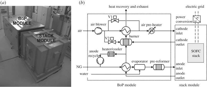
The system used in the study is a 10 kW SOFC system. It consists of two interconnected modules, i.e. balance of plant (BoP) and stack module. The BoP module includes blowers, heaters, pipes, heat exchangers, etc. The main role of the BoP is to supply the stack module with the corresponding amount of appropriately conditioned fuel. The stack module consists of 80 fuel cells, stacked one on top of another. The stack is enclosed in a thermally insulated housing since the cells operate at high temperatures. Water–gas shift (WGS), steam-methane reforming (SMR) and hydrogen-oxidation reactions take place inside the stack to produce heat, H₂O and electrical power. Figure 1 shows a schematic of the system on which the experiment was performed and a photograph of the actual system. Air (containing oxygen) is fed by air blower to the cathode inlet of the stack. Methane (natural gas, NG) is passed through a reformer in order to get hydrogen, which is delivered to the anode inlet. The remaining fuel in the cathode outlet is recycled for the sake of higher efficiency.

Figure 1.

The SOFC power-generating unit installed at VTT (a) and its schematic representation (b) [21].

During the test, various operational parameters were manipulated for a complete characterization of the system.

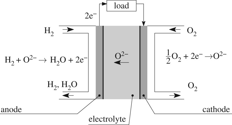
The principle of operation for a single-cell is illustrated in figure 2. The electrolyte transports oxygen ions O²⁻ from the cathode to the anode, while at the same time preventing direct contact between the anode and cathode chambers. The ions are formed via the oxygen-reduction reaction at the cathode, which is continuously fed with oxygen. On the other side, at the anode, the O²⁻ ions react with hydrogen in the process of hydrogen oxidation. In addition to H₂O, two electrons and some heat are released. The electrons travel through the external load to reach the cathode, where they participate in the oxygen-reduction reaction.

Figure 2.

Basic principles of a SOFC and its essential components.

Theoretically, a single SOFC's voltage can reach 1.2 V, depending on the temperature, pressure and gas composition. Consequently, for higher power outputs, typically several fuel cells are connected in parallel to form a fuel cell stack.

Since the SOFCs operate at high temperatures, the stack is usually enclosed in an insulated housing to reduce the heat losses. The stack then connects with a BoP module, which carries out the pre-treatment of the incoming gases. The BoP consists of different interconnected components, such as heat-exchangers, blowers, fuel reformers, pipes, valves, etc.

(b). Nonlinear stack model

The dynamics of the stack can be described as a lumped parameter model with the energy balance written as follows [22]:

$$K_s\frac{\mathrm{d}T}{\mathrm{d}t}={\dot{E}}_{\mathrm{in}}(T_{\mathrm{in}})-{\dot{E}}_{\mathrm{out}}(T)-IU,$$ 3.1

where T is the outlet-gas temperature, ${\dot{E}}_{\mathrm{in}}$ and ${\dot{E}}_{\mathrm{out}}$ denote the energy flows in and out of the stack, respectively, K_s denotes the lumped heat capacity of the stack, U is the stack voltage and I is the load current. The energy flows ${\dot{E}}_{\xi }$ are defined as [22]:

$${\dot{E}}_{\xi }=\sum _i{\dot{n}}_i^{\xi }{h}_i(T^{\xi }),$$ 3.2

where ${\dot{n}}_i^{\xi }$ denotes the molar flow of the ith gas component, i∈{H₂, H₂O, CH₄, CO, CO₂, O₂, N₂}, at corresponding locations where ξ∈{in, out}, i.e. the stack inlet/outlet, and with corresponding temperatures T^ξ_i, and h_i is the enthalpy of the gas.

The SMR, WGS and hydrogen-oxidation reactions are considered to be in thermodynamic equilibrium. This assumption is easily justified and often employed in the modelling of SOFC systems. A detailed discussion of these issues is available in [23]. Furthermore, total methane reforming is assumed for this application [24]. In turn, the molar flow $\dot{n}$ of the ith gas component at the anode outlet ${\dot{n}}_i^{\mathrm{out}}$ can be calculated from the inlet molar flow ${\dot{n}}_i^{\mathrm{in}}$ and the extent of the SMR x, WGS y, and the hydrogen-oxidation reactions z:

$$\begin{array}{l}\begin{array}{rl}& {\dot{n}}_{{\mathrm{H}}_2\mathrm{O}}^{\mathrm{out}}={\dot{n}}_{{\mathrm{H}}_2\mathrm{O}}^{\mathrm{in}}-x-y+z\\ & {\dot{n}}_{{\mathrm{H}}_2}^{\mathrm{out}}={\dot{n}}_{{\mathrm{H}}_2}^{\mathrm{in}}+3x+y-z\\ & {\dot{n}}_{{\mathrm{CH}}_4}^{\mathrm{out}}={\dot{n}}_{{\mathrm{CH}}_4}^{\mathrm{in}}-x\\ & {\dot{n}}_{\mathrm{CO}}^{\mathrm{out}}={\dot{n}}_{\mathrm{CO}}^{\mathrm{in}}+x-y\\ \mathrm{and}& {\dot{n}}_{{\mathrm{CO}}_2}^{\mathrm{out}}={\dot{n}}_{{\mathrm{CO}}_2}^{\mathrm{in}}+y.\end{array}\begin{array}{rl}& {\dot{n}}_{{\mathrm{N}}_2}^{\mathrm{out}}={\dot{n}}_{{\mathrm{N}}_2}^{\mathrm{in}}\\ & z=\frac{N_{0}I}{n_{e}F},\\ & K_{wgs}(T)=\frac{{\dot{n}}_{{\mathrm{CO}}_2}^{\mathrm{out}}\cdot {\dot{n}}_{{\mathrm{H}}_2}^{\mathrm{out}}}{{\dot{n}}_{\mathrm{CO}}^{\mathrm{out}}\cdot {\dot{n}}_{{\mathrm{H}}_2\mathrm{O}}^{\mathrm{out}}},\end{array}\end{array}\}$$ 3.3

where N₀ is the number of cells, F is Faraday's constant, n_e is the number of free electrons. K_wgs is the temperature-dependent WGS equilibrium constant:

$$\log K_{wgs}=A{T}^4+B{T}^3+C{T}^2+DT+E.$$ 3.4

Details about the parameters A, B, C, D and E are discussed in [25]. Furthermore, in K_wgs from (3.3) all the components are gases. The concentration of each gas component is assumed to be directly proportional to its flow rates. Moreover, it can be shown that the methane-conversion rate is nearly 100% [26], hence $x={\dot{n}}_{{\mathrm{CH}}_4}^{\mathrm{in}}$. Therefore, to have a more simplified model, the SMR is dropped from the equilibrium calculation. Finally, y is the only unknown and can be easily calculated from the K_wgs equation, see [24] for details. Note that usually there is also some nitrogen present on the fuel side. Ideally, nitrogen does not react, hence ${\dot{n}}_{{\mathrm{N}}_2}^{\mathrm{out}}={\dot{n}}_{{\mathrm{N}}_2}^{\mathrm{in}}$.

The Nernst voltage of a single cell U₀ is evaluated by employing [27, p. 269]:

$$U_0=1.2586-0.000252T+\frac{RT}{2F}\ln \frac{p_{{\mathrm{H}}_2}{p}_{o_2}^{0.5}}{p_{{\mathrm{H}}_2\mathrm{O}}},$$ 3.5

where R is the universal gas constant, p_H2, p_O2 and p_H2O are the hydrogen, oxygen and water-vapour partial pressures inside the stack. The partial pressures of the gases inside the stack are approximated from the input/output partial pressures, which can be easily evaluated from (3.3)

$$p_j=\frac{1}{2}(\frac{{\dot{n}}_j^{\mathrm{in}}}{{\dot{n}}_{\mathrm{tot}}^{\mathrm{in}}}+\frac{{\dot{n}}_j^{\mathrm{out}}}{{\dot{n}}_{\mathrm{tot}}^{\mathrm{out}}}),$$

where j∈{H₂, H₂O} and ${\dot{n}}_{\mathrm{tot}}^{\mathrm{in}/\mathrm{out}}$ are the total anode inlet/outlet molar flows. On the cathode side the oxygen partial pressure p_O2 is calculated in the same manner.

The temperature variation of the lumped Ohmic ASR of a single cell can be expressed by the second-order Steinhart–Hart equation [27,28]:

$$r=\gamma \exp \left[\frac{30\hspace{0.17em}000}{R}(\frac{1}{T}-\frac{1}{T_0})\right],$$ 3.6

where γ is the ohmic ASR at the reference temperature T₀.

The ASR model (3.6) is fairly simple. It only considers the ASR dependence on the temperature, and it is only used to model the SOFC voltage dependence on the current (or Ohmic losses), in a linear fashion in (3.7), whereas the total cell losses include the diffusion and activation polarization losses. However, as discussed in [29], the full model of the ASR is parametrized by many different material properties, e.g. porosity and tortuosity. Moreover, the ASR also depends on the operating conditions, such as different gas mixtures, which are usually kept relatively steady during the SOFC's operating time.

Therefore, the main assumption here is that the temperature has the dominant impact on the ASR when considering the nominal operating conditions.

The stack voltage U can be expressed as

$$U=N_0(U_0-\mathrm{ASR}\cdot \frac{I}{A}),$$ 3.7

where A is the active area of a single cell.

The lumped dynamic model of the stack reads as follows:

$$\begin{array}{rl}{K}_s\frac{\mathrm{d}T}{\mathrm{d}t}& ={\dot{E}}_{\mathrm{in}}(T_{\mathrm{in}})-{\dot{E}}_{\mathrm{out}}(T)\\ & -I{N}_0(1.2586-0.000252T+\frac{RT}{2F}\ln \frac{p_{{\mathrm{H}}_2}{p}_{o_2}^{0.5}}{p_{{\mathrm{H}}_2\mathrm{O}}}-\gamma \exp \left[\frac{30\hspace{0.17em}000}{R}(\frac{1}{T}-\frac{1}{T_0})\right]\cdot \frac{I}{A}).\end{array}$$ 3.8

It should be noted that in order to keep the model (3.8) straightforward, many simplifications had to be made. Hence, only the dynamics of the thermal processes was taken into account, while the rest was assumed to be static. The distributed nature of the process is also ignored, hence the lumped dynamic model of the SOFC stack.

(c). Degradation dynamics and coupling functions

In [30,31], a range of durability experiments were performed on anode-supported SOFCs at different temperatures, current densities and several values of fuel utilization (between 75% and 85%). The test matrix enclosed the temperature points 950, 850 and 750°C and current densities were chosen between 0.2 and 1.9 A cm⁻². Degradation rates were shown to be mainly dependent on the cell polarization. Additional analyses revealed that cathode degradation was the dominant contribution to the degradation at higher current densities and lower temperatures. The anode was found to contribute more to the degradation at higher temperatures. Generally, the degradation rates obtained were lower at higher operating temperatures, even at higher current densities.

From the results of the experiments published in [32] an empirical model relating the degradation rate r_d, on the one hand, and fuel utilization FU, temperature T and current density j, on the other, was obtained:

$$r_d(FU,T,j)=\frac{0.59\mathit{F}\mathit{U}+0.74}{1+{\mathrm{e}}^{((T-1087)/(22.92))}}({\mathrm{e}}^{2.64j}-1).$$ 3.9

The degradation rate r_d describes the incremental increase in the Ohmic losses of the stack.

Clearly, the values of the parameters in (3.9) only hold for the specific single cell used therein. Here, we suppose that the model can be scaled up for the stack of cells, which means the same model structure could be used. The model parameters will be updated from data by the optimization procedure.

Given the specifics of the experimental set-up used in this study, we do not operate with the current density j but the current I itself. After taking into account that the fuel utilization is more-or-less constant during the experiment, we propose the following coupling function, defined by the vector of parameters θ = (a b c)^T

$$r_d(T,I,\mathit{\theta })=\frac{a}{1+{\mathrm{e}}^{((T-T_0)/b)}}({\mathrm{e}}^{cI}-1),$$ 3.10

where T₀ is a known value.

The degradation model (3.10) can be coupled with the stack model (3.8) to form a coupled dynamic nonlinear state space model

$$\frac{\mathrm{d}T}{\mathrm{d}t}=f(\bullet ,\gamma ,T)$$ 3.11

and

$$\frac{\mathrm{d}\gamma }{\mathrm{d}t}=r_d(\bullet ,\gamma ,T),$$ 3.12

where • is used to omit an explicit listing of all the influential variables and only focus on the coupling dependencies.

The coupled differential equations (3.11) and (3.12) describe the system's nominal dynamics and the hidden dynamics of the degradation, respectively.

(d). Problem statement and solution options

Let us now introduce the system state vector x = (T γ)^T, the vector of inputs $\mathit{u}=({\dot{n}}_{\mathrm{air}}\hspace{0.17em}{\dot{n}}_{{\mathrm{CH}}_4}\hspace{0.17em}\mathrm{U})$ and the measurable output y = T. After the discretization

$$\begin{array}{rl}& \frac{\mathrm{d}T}{\mathrm{d}t}{|}_{t=t_k}\approx \frac{T(t_{k+1})-T(t_k)}{\mathrm{\Delta }t}\\ \mathrm{and}& \frac{\mathrm{d}\gamma }{\mathrm{d}t}{|}_{t=t_k}\approx \frac{\gamma (t_{k+1})-\gamma (t_k)}{\mathrm{\Delta }t},\end{array}\}$$ 3.13

where Δt stands for the sampling rate, we obtain the system of difference equations, which can be represented in the most general form

$${\mathit{x}}_{k+1}=\mathit{g}({\mathit{x}}_k,{\mathit{u}}_k,\mathit{\theta })+{\mathit{\chi }}_k$$ 3.14

and

$${\mathit{y}}_k=\mathit{h}({\mathit{x}}_k,{\mathit{u}}_k,\mathit{\theta })+{\mathit{\zeta }}_k,$$ 3.15

where χ_k and ζ_k are the noise terms that encompass random disturbances in the process, along with the modelling error. Here, g(x_k, u_k) are nonlinear state-transition equations of the model, and h(x_k, u_k) represents the nonlinear output equations. The terms χ_k and ζ_k are the zero mean Gaussian noise with the corresponding covariance matrices. The time step is denoted with k.

(i). Solution option 1: combined state and parameter estimation.

The essence of the idea is to take the measurable input and output realizations $\mathcal{D}=\{{\mathit{y}}_1,\dots ,{\mathit{y}}_T,{\mathit{u}}_1\cdots ,{\mathit{u}}_T\}$ to evaluate the unknown vector of the parameters θ along with the hidden states x₁, …, x_T. This way is computationally rather cumbersome. Indeed, no matter whether the maximum likelihood or the Bayesian approach is used, the evaluation of the inevitable likelihood is non-trivial

$$p({\mathit{y}}_1,\dots ,{\mathit{y}}_T,{\mathit{x}}_1\dots ,{\mathit{x}}_T|\mathit{\theta },{\mathit{x}}_0)=p({\mathit{x}}_0|\mathit{\theta })\prod _{k=0}^{T-1}p({\mathit{x}}_{k+1}|{\mathit{x}}_k,\mathit{\theta })\prod _{k=1}^{T}p({\mathit{y}}_k|{\mathit{x}}_k,\mathit{\theta }).$$ 3.16

Since the model is nonlinear, an analytical evolution of the moments of the pdfs (as is the case in linear models) is not possible. Instead, the conditional densities could be approximated numerically by drawing samples from the corresponding distributions. To draw samples from the posterior, we need only to specify a tractable calculation of the joint probability p(x_k+1|x_k, θ) and p(y_k|x_k, θ). The best-known Markov chain Monte Carlo (MCMC) algorithms include, for instance, the Metropolis–Haistings algorithm, the Gibbs sampler, slice sampling and the Hamilton Monte Carlo [33].

Unfortunately, the Monte Carlo-based methods suffer from the curse of dimensionality. For multi-dimensional models, the number of samples required to properly describe the shape of the distribution function increases almost exponentially with the dimension of the model.

(ii). Solution option 2: parameter estimation.

First, we will show that a simplification of the dynamical model (3.11) could reduce the complexity of the original problem, but result in high-quality solutions. In that respect, note that the degradation dynamics (3.12) is significantly slower than the process dynamics (3.11). Indeed, the latter runs on an hourly scale, while the former usually takes months, which is several orders of magnitude slower. Consequently, on the local time scale, the state of the degradation could be considered constant. Based on that observation, the nominal dynamic model (3.8) could be rewritten as follows:

$$K_s\frac{\mathrm{d}T}{\mathrm{d}t}={\mathcal{Q}}_1(t)-\gamma {\mathcal{Q}}_2(t),$$ 3.17

where ${\mathcal{Q}}_1(t)$ and ${\mathcal{Q}}_2(t)$ are expressions that can be computed from the available signals. By using the Savitzky–Golay filter, the derivative dT/dt is estimated numerically. Hence, the evaluation of γ on the local scale can be formulated as the least-squares problem taken on the regression

$$-{\mathcal{Q}}_2(t)\gamma =K_s\frac{\mathrm{d}\hat{T}}{\mathrm{d}t}-{\mathcal{Q}}_1(t),$$ 3.18

from which γ can be evaluated based on samples from the local time window. Hence, we obtain the evaluated values of the realization of the stochastic process associated with the degradation through γ. With numerical differentiation on a slow time scale, we obtain the nonlinear regression problem (3.18) fully defined.

4. Variational Bayesian approach to the parameter estimation of the nonlinear coupling functions

(a). The idea

Assume $\mathcal{D}$ are measured data, i.e. the realization of a set of measurable random variables. In our case, those are the estimated derivatives dγ/dt and θ is an unknown random vector (in our case θ = (a b c)^T). The Bayesian framework provides a way to elicit the full information from the data, of course, at the expense of additional computational complexity.

The distribution of unknown θ given the dataset $\mathcal{D}$ is evaluated by means of the Bayes rule

$$p(\mathit{\theta }|\mathcal{D})=\frac{p(\mathcal{D}|\mathit{\theta })p(\mathit{\theta })}{p(\mathcal{D})}=\frac{p(\mathcal{D}|\mathit{\theta })p(\mathit{\theta })}{\int p(\mathcal{D}|\mathit{\theta })p(\mathit{\theta })d\mathit{\theta }}.$$ 4.1

The evaluation of the denominator can easily become intractable in higher-dimensional problems, thereby rendering the computation of the exact posterior distribution practically impossible. There are several approaches that could overcome these difficulties, the most commonly used being MCMC and the variational Bayesian inference methods. Central to the both approaches is the evaluation of the normalization factor $p(\mathcal{D})$.

(b). Variational Bayesian methods

The main idea behind the variational methods is to find some approximation distribution¹ q(θ;λ) as close as possible to the true posterior distribution

$$q(\mathit{\theta };\mathit{\lambda })\approx p(\mathit{\theta }|\mathcal{D}).$$ 4.2

The aim is to find the setting of the parameters λ that make q as close as possible to the posterior of interest. Obviously, the distribution q(θ;λ) should be relatively easy and more tractable for inference. To evaluate the dissimilarity between the two distributions q(θ;λ) and $p(\mathit{\theta }|\mathcal{D})$, Kullback–Leibler (KL) divergence is used [34]:

$$\begin{array}{rl}KL(q(\mathit{\theta };\mathit{\lambda })||p(\mathit{\theta }|\mathcal{D}))& =\int q(\mathit{\theta };\mathit{\lambda })\log \frac{q(\mathit{\theta };\mathit{\lambda })}{p(\mathit{\theta }|\mathcal{D})}\mathrm{d}\theta \\ & =-\int q(\mathit{\theta };\mathit{\lambda })\log \frac{p(\mathit{\theta }|\mathcal{D})}{q(\mathit{\theta };\mathit{\lambda })}\mathrm{d}\theta \\ & =-\int q(\mathit{\theta };\mathit{\lambda })\log (\frac{p(\mathit{\theta }|\mathcal{D})}{q(\mathit{\theta };\mathit{\lambda })}\cdot \frac{p(\mathcal{D})}{p(\mathcal{D})})\mathrm{d}\theta \\ & =-\int q(\mathit{\theta };\mathit{\lambda })\log \frac{p(\mathit{\theta },\mathcal{D})}{q(\mathit{\theta };\mathit{\lambda })}d\theta +\int q(\mathit{\theta };\mathit{\lambda })\log \hspace{0.17em}p(\mathcal{D})\mathrm{d}\theta \\ & =-\underset{L(\mathit{\lambda })}{\underbrace{\int q(\mathit{\theta };\mathit{\lambda })\log \frac{p(\mathcal{D}|\mathit{\theta })p(\mathit{\theta })}{q(\mathit{\theta })}\mathrm{d}\mathit{\theta }}}+\log p(\mathcal{D})\underset{1}{\underbrace{\int q(\mathit{\theta };\mathit{\lambda })\mathrm{d}\mathit{\theta }}}\end{array}$$ 4.3

$$\begin{array}{r}\\ & =-L(\mathit{\lambda })+\log p(\mathcal{D}),\end{array}$$ 4.4

where L(λ) is referred to as evidence lower bound (ELBO). From (4.4), it follows that

$$L(\mathit{\lambda })=\log p(\mathcal{D})-KL(q(\mathit{\theta };\mathit{\lambda })||p(\mathit{\theta }|\mathcal{D})).$$ 4.5

Since the KL divergence is always ≥0 it turns out that $L\le \log p(\mathcal{D})$, i.e. L is the lower bound of the pdf of the observations. Note that $\log p(\mathcal{D})$ does not depend on the variational parameters λ, we can minimize the KL divergence (4.4) by minimizing the first expression ELBO on the right-hand side. Note also that in the expression for ELBO p(θ) is known prior and $p(\mathcal{D}|\mathit{\theta })$ is the system model, which can be easily computed by sampling from the distribution of θ and the Monte Carlo simulation.

(c). The stochastic gradient optimization

Now we have a variational family of approximations q(θ;λ) parametrized by λ. ELBO is minimized using a stochastic gradient descent with adaptive and decreasing step sizes. Since the criterion is defined on a sample of random variables, it is itself a random variable. Consequently, instead of exact gradients (as in a classic gradient descent) we use gradients approximated by Monte Carlo methods. The approach is referred to as ADAM [35] (the acronym stands for adaptive moment estimation).

The algorithm adaptively finds the individual learning rates for each component λ^(s), s = 1, …, K of the vector λ by estimating the first moment m^(s)_t and the second moment v^(s)_t of the gradient. To do so, ADAM uses exponentially moving averages, computed on the gradient evaluated on a current mini-batch:²

$$\begin{array}{rl}& m_t={\beta }_1{m}_{t-1}+(1-{\beta }_1)g_t\\ \mathrm{and}& v_t={\beta }_2{v}_{t-1}+(1-{\beta }_2)g_t^2\end{array}\}$$ 4.6

with t the number of iterations, m_t and v_t the estimated first and second moments and β_i, i∈1, 2 being the parameters of the moving average. For the parameters β_i, ADAM uses the default values of 0.9 and 0.999, respectively. The initialization with m₀ = 0 and v₀ = 0 turns not to have an important impact on the convergence. The vector of gradients evaluated on the data window ${\mathcal{D}}_w$ reads as follows:

$$\mathit{g}={(g^{(1)},\dots ,g^{(K)})}^{\mathrm{T}}={\mathbf{\nabla }}_{\mathit{\lambda }}{L}_{{\mathcal{D}}_w}(\mathit{\lambda }).$$ 4.7

Since m and v are estimates of the first and second moments, it is desirable that they have the following property:

$$\begin{array}{rl}& E\{m_t\}=E(g_t)\\ \mathrm{and}& E\{v_t\}=E(g_t^2).\end{array}\}$$ 4.8

These are the conditions for unbiased estimates. Note that the recursion (4.6) in the case of the first moment and at the iteration t looks as follows:

$$m_t=(1-{\beta }_1)\sum _{i=1}^t{\beta }_1^{t-i}{g}_i.$$ 4.9

However, there is some bias present in that estimate. If we take the expected values on both sides we obtain

$$\begin{array}{rl}{E}_{\mathit{\lambda }}[m_t]& =(1-{\beta }_1)\sum _{i=1}^t{\beta }_1^{t-i}{E}_{\mathit{\lambda }}[g_i]\\ & \approx (1-{\beta }_1)\left(\sum _{i=1}^t{\beta }_1^{t-i}\right)E_{\mathit{\lambda }}[g_t]\\ & =(1-{\beta }_1^t)E_{\mathit{\lambda }}[g_t].\end{array}$$ 4.10

ADAM evaluates the estimates of the moments of the gradients with a simple bias correction

$${\hat{m}}_t=\frac{m_t}{1-{\beta }_1^t},$$ 4.11

and in a similar manner

$${\hat{v}}_t=\frac{v_t}{1-{\beta }_2^t}.$$ 4.12

The algorithm adjusts the optimization step individually for each parameter

$${\lambda }_t^{(s)}={\lambda }_{t-1}^{(s)}-\eta \frac{{\hat{m}}_t^{(s)}}{\sqrt{{\hat{v}}_t^{(s)}}+\eta },$$ 4.13

with η = 0.001 [35].

ADAM is entirely heuristic and has proved efficient in a broad range of applications. Its implementation in Python is very simple and little computational time is needed to obtain the optimal solution. However, as is the case with heuristic optimization algorithms, the convergence might not be guaranteed in all cases. In the original paper [35], it is proven that ADAM converges to the global minimum in the convex settings. In spite of the fact that some errors in the original convergence analysis have been spotted afterwards by Bock et al. [36], they managed to prove that the algorithm converges.

5. Experimental evaluation on the solid-oxide fuel cell system

The dataset $\mathcal{D}$, thoroughly discussed in [24], consists of over 100 signals acquired through the installed instrumentation. For instance, the gas composition is measured at five different locations, at the stack inlets and outlets, in the BoP before and after the fuel reforming, etc. The temperatures are measured at the mixture point, i.e. at the recycling point in the BoP, as well as at the entry points to the system as a whole and the entry points to the stack.

(a). The experiment

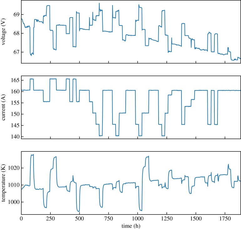
During the experiment, the temperature varied around T₀ = 1010 K, which is the constant that appears in model (3.10). The profiles of the temperature, current and voltage shown in figure 3 clearly indicate that the system has been operating in non-stationary conditions all the time. This profile has two distinctive features: rapid changes (on the scale of several hours) and a slow, positive trend throughout the experiment.

Figure 3.

Measured stack voltage, current and the outlet stack temperature during the experiment. (Online version in colour.)

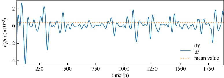
The system dynamics is described by the dynamic model (3.8). Variations in the outlet-gas temperature are due to the variations of several input variables, like load current, gas composition at the system inlets, etc. Based on local regression (3.18), the evolution of the degradation rate dγ/dt is evaluated and shown in figure 4. Note that the mean of the stochastic evolution of dγ/dt is slightly positive, meaning the degradation is progressing on a broader time scale. Local variations are due to imperfections in the nominal model (3.8).

Figure 4.

Estimated rate of change of ASR in the SOFC stack [7]. (Online version in colour.)

(b). Variational Bayesian inference of the nonlinear coupling function

Let us now analyse the performance of the variational Bayesian inference of the nonlinear coupling function.

When selecting the approximating distribution q for the posterior, we decided to treat the parameters a, b, c as statistically independent normal variables. Hence

$$q(\mathit{\theta };\mathit{\lambda })=\mathcal{N}({\mu }_a,{\sigma }_a^2)\cdot \mathcal{N}({\mu }_b,{\sigma }_b^2)\cdot \mathcal{N}({\mu }_c,{\sigma }_c^2)$$ 5.1

with the vector of hyperparameters λ = ({μ_i σ²_i, i = 1, 2, 3}^T) The proposed method is numerically implemented in Python code by using the library pyro.ai [37].

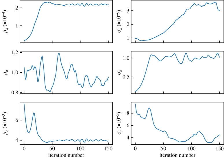
Figure 5 shows the convergence of a stochastic optimization run at a particular time point t = 412 h. Relatively rapid convergence towards the statistical means can be observed. The fluctuation in the parameter μ_b seems to indicate the relatively low sensitivity of the criterion function L(λ) with respect to that particular parameter.

Figure 5.

Estimated means and variances of the hyperparameters λ during an optimization run. The means of the approximating Gaussians are in the left-hand column, while variances are in the right-hand column. A relatively rapid convergence rate can be observed. (Online version in colour.)

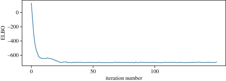
Figure 6 shows the evolution of ELBO during the optimization run, indicating extremely rapid convergence. On a typical PC, it took about 15 s of computational time.

Figure 6.

Evidence lower bound (ELBO) over iterations showing rapid convergence. (Online version in colour.)

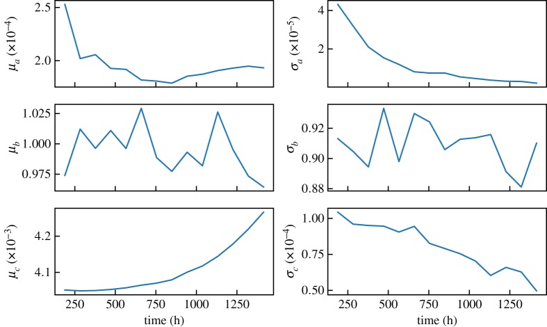
Let us now see the evolution of the hyperparameters λ over time (figure 7). The first two hyperparameters μ_a and μ_b do not change significantly over time, hence the same holds true for a and b. However, that is not the case with the parameter c, which increases with time. This could be interpreted so that with the progressing degradation the impact of the current on the degradation rate increases. If we want to slow down the degradation, decreasing the current could be an option.

Figure 7.

The evolution of the hyperparameters λ during the experiment. (Online version in colour.)

(c). Comparison of the predictive performance of two degradation models

In order to analyse the benefit of nonlinear coupling functions, the results are compared with those obtained with a simple local linear model for the dynamics of γ proposed by [7]. For the sake of clarity, let us denote the two models by ${\mathcal{M}}_1$ and ${\mathcal{M}}_2$ as follows:

$${\mathcal{M}}_1:{\gamma }_{k+1}={\gamma }_k+\mathrm{\Delta }t\frac{a}{1+{\mathrm{e}}^{((T_k-T_0)/b)}}({\mathrm{e}}^{c{I}_k}-1)+d$$ 5.2

and

$${\mathcal{M}}_2:{\gamma }_{k+1}={\gamma }_k+d,$$ 5.3

where the stochastic term d models the trend in γ. The second model is obviously simpler and is updated by local linear regression.

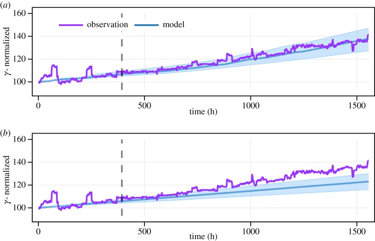
The predictive pdf $p({\gamma }_{t+r}|{\mathcal{D}}_t)$ is evaluated with a Monte Carlo simulation, as described in [7]. Figure 8 summarizes an important result of the paper. Figure 8a shows the predicted evaluation of γ in the case that the degradation dynamics is modelled with ${\mathcal{M}}_1$. Figure 8b shows the results with a simpler black-box structure ${\mathcal{M}}_2$. By taking into account that the parameters of both models were estimated on the same dataset, the benefit of employing a more complex structure ${\mathcal{M}}_1$ is apparent. Namely, the model that employs prior knowledge through a coupling function (5.2) predicts the evolution of the γ with a greater precision than the one employing (5.3). Therefore, using the model (5.2) could improve the results obtained in [7].

Figure 8.

Comparison of the model where the degradation dynamics is modelled through the coupling function (5.2), and where a simpler black-box structure (5.3) is adopted. The dashed vertical separates the dataset on the identification (left) and validation (right) parts. (a) Experimental validation of the model (5.2). (b) Experimental validation of the model (5.3). (Online version in colour.)

A remark

Finally, it is important to stress that the successful application of the prior nonlinear coupling function depends on whether the degradation mechanism is correctly diagnosed. If the diagnosis turns out to be wrong, it is likely that the prediction will be poor. Therefore, we have to discuss that aspect, which is of relevance when the application comes into play. It is known that completely different detrimental phenomena produce similar symptoms. Hence, the first question is whether we are able to unambiguously reveal which mechanism is exactly under way. That is not an easy task because of

• —limited capabilities of the existing diagnostic methods along with the limited standard instrumentation accompanying the deployed systems,
• —there are only a few degradation mechanisms for which phenomenological coupling functions are available,
• —often several degradation mechanisms take place at the same time, rather than only a single one, which additionally complicates the diagnosis.

Instead of using one coupling function it might be worth thinking of using an ensemble of candidate models and favour those that have better performance.

6. Conclusion

In this paper, a nonlinear coupling function is used to describe the link between the SOFC's operational dynamics and the slowly evolving degradation process. The contribution of the paper is threefold. Firstly, it seems to be the first attempt to handle the estimation of a nonlinear coupling function with the variational Bayesian approximation. It is demonstrated that the approach exhibits a remarkable convergence performance at a relatively low computational load. Computations required by the MCMC approaches would require at least an order of magnitude more computational load for a questionable extra benefit. The positive experience seems stimulating enough to extend the approach to other application domains with a comparable problem setup. An example is the prognosis of the RUL of rotational drives. We showed in our earlier work, cf. [38], that progressive damage in the contact surfaces can be modelled as a nonlinear stochastic process.

The second contribution is related to the demonstration that the use of more prior knowledge, even at the expense of a more complex model structure, can bring benefits in terms of a greater accuracy for the predicted degradation trends.

The third contribution concerns the ability of the proposed algorithm to operate reliably in non-stationary operating conditions, which is of great importance for the continuous condition monitoring of SOFCs in realistic applications. The results based on the experimental data clearly support the above assertions.

Our follow-up will concentrate on using several candidate models with a different structure at the same time. Hence, it is expected that the prognostics will appear to be more robust to the inaccurate diagnosis of the true degradation mechanism.

Data accessibility

This article has no additional data.

Competing interests

We declare we have no competing interests.

Funding

The work was supported by the Slovenian Research Agency through programme P2-0001 and project J2-9441, and in part by the Fuel Cells and Hydrogen Joint Undertaking (FCH JU) under grant agreement no. 735918 (INSIGHT project). B.D. acknowledges EPSRC grant no. EP/M006298/1, and P.B. the Erasmus grant SI NOVO ME05 for financial support during their visits to the Physics Department, Lancaster University, where the work was initiated.

References

- 1.Aguilo-Rullan A, Atanasiu M, Biebuyck B, Lymperopoulos N, Marenco C, Tsimis D. 2017. The status of SOFC and SOEC R&D in the European fuel cell and hydrogen joint undertaking programme. ECS Trans. 78, 41–61. ( 10.1149/07801.0041ecst) [DOI] [Google Scholar]
- 2.Anandakumar G, Li N, Verma A, Singh P, Kim JH. 2010. Thermal stress and probability of failure analyses of functionally graded solid oxide fuel cells. J. Power Sources 195, 6659–6670. ( 10.1016/j.jpowsour.2010.04.017) [DOI] [Google Scholar]
- 3.Iwata T. 1996. Characterization of Ni-YSZ anode degradation for substrate-type solid oxide fuel cells. J. Electrochem. Soc. 143, 1521–1525. ( 10.1149/1.1836673) [DOI] [Google Scholar]
- 4.Iwanschitz B, Holzer L, Mai A, Schütze M. 2012. Nickel agglomeration in solid oxide fuel cells: the influence of temperature. Solid State Ionics 211, 69–73. ( 10.1016/j.ssi.2012.01.015) [DOI] [Google Scholar]
- 5.de Haart L, Neumann A, Menzler N, Vinke I. 2011. Is chromium poisoning of LSM cathodes avoidable? ECS Trans. 36, 2027–2033. ( 10.1149/1.3570193) [DOI] [Google Scholar]
- 6.Koh JH, Yoo YS, Park JW, Lim HC. 2002. Carbon deposition and cell performance of Ni-YSZ anode support SOFC with methane fuel. Solid State Ionics 149, 157–166. ( 10.1016/S0167-2738(02)00243-6) [DOI] [Google Scholar]
- 7.Dolenc B, Boškoski P, Stepančič M, Pohjoranta A, Juričić Đ. 2017. State of health estimation and remaining useful life prediction of solid oxide fuel cell stack. Energy Convers. Manag. 148, 993–1002. ( 10.1016/j.enconman.2017.06.041) [DOI] [Google Scholar]
- 8.Stankovski T, Pereira T, McClintock PVE, Stefanovska A. 2017. Coupling functions: universal insights into dynamical interaction mechanisms. Rev. Mod. Phys. 89, 045001 ( 10.1103/RevModPhys.89.045001) [DOI] [Google Scholar]
- 9.Recknagle K, Williford R, Chick L, Rector D, Khaleel M. 2003. Three-dimensional thermo-fluid electrochemical modeling of planar SOFC stacks. J. Power Sources 113, 109–114. ( 10.1016/S0378-7753(02)00487-1) [DOI] [Google Scholar]
- 10.Nakajo A, Wuillemin Z, Herle JV, Favrat D. 2009. Simulation of thermal stresses in anode-supported solid oxide fuel cell stacks. Part I: probability of failure of the cells. J. Power Sources 193, 203–215. ( 10.1016/j.jpowsour.2008.12.050) [DOI] [Google Scholar]
- 11.Liu L, Kim GY, Chandra A. 2010. Modeling of thermal stresses and lifetime prediction of planar solid oxide fuel cell under thermal cycling conditions. J. Power Sources 195, 2310–2318. ( 10.1016/j.jpowsour.2009.10.064) [DOI] [Google Scholar]
- 12.Cronin JS, Wilson JR, Barnett SA. 2011. Impact of pore microstructure evolution on polarization resistance of Ni-Yttria-stabilized zirconia fuel cell anodes. J. Power Sources 196, 2640–2643. ( 10.1016/j.jpowsour.2010.10.084) [DOI] [Google Scholar]
- 13.Lee YH, Muroyama H, Matsui T, Eguchi K. 2014. Degradation of nickel–yttria-stabilized zirconia anode in solid oxide fuel cells under changing temperature and humidity conditions. J. Power Sources 262, 451–456. ( 10.1016/j.jpowsour.2014.03.031) [DOI] [Google Scholar]
- 14.Larrain D. 2006. Simulation of SOFC stack and repeat elements including interconnect degradation and anode reoxidation risk. J. Power Sources 161, 392–403. ( 10.1016/j.jpowsour.2006.04.151) [DOI] [Google Scholar]
- 15.Hallström S, Halvarsson M, Höglund L, Jonsson T, Ågren J. 2013. High temperature oxidation of chromium: kinetic modeling and microstructural investigation. Solid State Ionics 240, 41–50. ( 10.1016/j.ssi.2013.02.017) [DOI] [Google Scholar]
- 16.Barelli L, Barluzzi E, Bidini G. 2016. Diagnosis methodology and technique for solid oxide fuel cells: a review. Int. J. Hydrog. Energy 38, 5060–5074. ( 10.1016/j.ijhydene.2013.02.024) [DOI] [Google Scholar]
- 17.Costamagna P, Rossi S, Pugliese F, Gugliotta F, Enrico A. 2015. FDI oriented simulation of an MSR reactor for application in SOFC systems. ECS Trans. 68, 3143–3150. ( 10.1149/06801.3143ecst) [DOI] [Google Scholar]
- 18.Greco A, Sorce A, Littwin R, Costamagna P, Magistri L. 2014. Reformer faults in SOFC systems: experimental and modeling analysis, and simulated fault maps. Int. J. Hydrogen Energy 39, 21 700–21 713. ( 10.1016/j.ijhydene.2014.09.063) [DOI] [Google Scholar]
- 19.Sarantaridis D, Atkinson A. 2007. Redox cycling of ni-based solid oxide fuel cell anodes: a review. Fuel Cells 7, 246–258. ( 10.1002/(ISSN)1615-6854) [DOI] [Google Scholar]
- 20.Debenjak A, Boškoski P, Musizza B, Petrovčič J, Juričić Đ. 2014. Fast measurement of proton exchange membrane fuel cell impedance based on pseudo-random binary sequence perturbation signals and continuous wavelet transform. J. Power Sources 254, 112–118. ( 10.1016/j.jpowsour.2013.12.094) [DOI] [Google Scholar]
- 21.Pohjoranta A, Halinen M, Pennanen J, Kiviaho J. 2015. Solid oxide fuel cell stack temperature estimation with data-based modeling - designed experiments and parameter identification. J. Power Sources 277, 464–473. ( 10.1016/j.jpowsour.2014.08.130) [DOI] [Google Scholar]
- 22.Marra D, Sorrentino M, Pohjoranta A, Pianese C, Kiviaho J. 2015. A lumped dynamic modelling approach for model-based control and diagnosis of solid oxide fuel cell system with anode off-gas recycling. ECS Trans. 68, 3095–3106. ( 10.1149/06801.3095ecst) [DOI] [Google Scholar]
- 23.Halinen M, Thomann O, Kiviaho J. 2012. Effect of anode off-gas recycling on reforming of natural gas for solid oxide fuel cell systems. Fuel Cells 12, 754–760. ( 10.1002/fuce.v12.5) [DOI] [Google Scholar]
- 24.Dolenc B, Vrečko D, Juričić Đ, Pohjoranta A, Pianese C. 2017. Online gas composition estimation in solid oxide fuel cell systems with anode off-gas recycle configuration. J. Power Sources 343, 246–253. ( 10.1016/j.jpowsour.2017.01.038) [DOI] [Google Scholar]
- 25.Massardo AF, Lubelli F. 2000. Internal reforming solid oxide fuel cell-gas turbine combined cycles (IRSOFC-GT): part A—cell model and cycle thermodynamic analysis. J. Eng. Gas Turbines Power 122, 27–35. ( 10.1115/1.483187) [DOI] [Google Scholar]
- 26.Huang K, Goodenough JB. 2009. Solid oxide fuel cell technology. principles, performance and operations. Boca Raton, FL: CRC Press. [Google Scholar]
- 27.Huang B, Qi Y, Murshed AM. 2013. Dynamic modelling and predictive control in solid oxide fuel cells: first principle and data-based approaches. Chichester, UK: John Wiley & Sons. [Google Scholar]
- 28.Marra D, Pianese C, Polverino P, Sorrentino M. 2016. Models for solid oxide fuel cell systems: exploitation of models hierarchy for industrial design of control and diagnosis strategies. Berlin, Germany: Springer. [Google Scholar]
- 29.Njodzefon JC, Klotz D, Krompa A, Webera A, Ivers-Tiffée E. 2013. Electrochemical modeling of the current-voltage characteristics of an SOFC in fuel cell and electrolyzer operation modes. J. Electrochem. Soc. 160, F313–F323. ( 10.1149/2.018304jes) [DOI] [Google Scholar]
- 30.Hagen A, Barfod R, Hendriksen PV, Liu Y, Ramousse S. 2006. Degradation of anode supported SOFCs as a function of temperature and current load. J. Electrochem. Soc. 153, A1165–A1171. ( 10.1149/1.2193400) [DOI] [Google Scholar]
- 31.Abreu-Sepulveda MA, Harun NF, Hackett G, Hagen A, Tucker D. 2014. Accelerated degradation for hardware in the loop simulation of fuel cell-gas turbine hybrid system. J. Fuel Cell Sci. Technol. 2, 1–17. ( 10.1115/1.4028953) [DOI] [Google Scholar]
- 32.Zaccaria V, Tucker D, Traverso A. 2016. A distributed real-time model of degradation in a solid oxide fuel cell, part i: model characterization. J. Power Sources 311, 175–181. ( 10.1016/j.jpowsour.2016.02.040) [DOI] [Google Scholar]
- 33.Barbu A, Zhu SC. 2019. Monte Carlo methods. London, UK: Springer. [Google Scholar]
- 34.Smidl V, Quinn A. 2006. The variational Bayes method in signal processing. Berlin, Germany: Springer. [Google Scholar]
- 35.Diederik P, Kingma JB. 2017 ADAM: a method for stochastic optimization. (http://arxiv.org/abs/quant-ph/1412.6980. )
- 36.Bock S, Goppold J, Weiss M. 2018 An improvement of the convergence proof of the ADAM-optimizer. (http://arxiv.org/abs/quant-ph/1804.10587. )
- 37.Bingham E, Chen JP, Jankowiak M, Obermeyer F, Pradhan N, Karaletsos T, Singh R, Szerlip P, Horsfall P, Goodman ND. 2019. Pyro: deep universal probabilistic programming. J. Mach. Learn. Res. 20, 1–6. [Google Scholar]
- 38.Boškoski P, Gašperin M, Juričić Đ. 2015. Bearing fault prognostics using Rényi entropy based features and Gaussian process model. Mech. Syst. Signal Process. 52–53, 327–337. ( 10.1016/j.ymssp.2014.07.011) [DOI] [Google Scholar]
Associated Data
This section collects any data citations, data availability statements, or supplementary materials included in this article.
Data Availability Statement