Opportunities and Limitations for Untargeted Mass Spectrometry Metabolomics to Identify Biologically Active Constituents in Complex Natural Product Mixtures

Abstract

Compounds derived from natural sources represent the majority of small-molecule drugs utilized today. Plants, owing to their complex biosynthetic pathways, are poised to synthesize diverse secondary metabolites that selectively target biological macromolecules. Despite the vast chemical landscape of botanicals, drug discovery programs from these sources have diminished due to the costly and time-consuming nature of standard practices and high rates of compound rediscovery. Untargeted metabolomics approaches that integrate biological and chemical datasets potentially enable the prediction of active constituents early in the fractionation process. However, data acquisition and data processing parameters may have major impacts on the success of models produced. Using an inactive botanical mixture spiked with known antimicrobial compounds, untargeted mass spectrometry-based metabolomics data were combined with bioactivity data to produce selectivity ratio models subjected to a variety of data acquisition and data processing parameters. Selectivity ratio models were used to identify active constituents that were intentionally added to the mixture, along with an additional antimicrobial compound, randainal (5), which was masked by the presence of antagonists in the mixture. These studies found that data-processing approaches, particularly data transformation and model simplification tools using a variance cutoff, had significant impacts on the models produced, either masking or enhancing the ability to detect active constituents in samples. The current study highlights the importance of the data processing step for obtaining reliable information from metabolomics models and demonstrates the strengths and limitations of selectivity ratio analysis to comprehensively assess complex botanical mixtures.

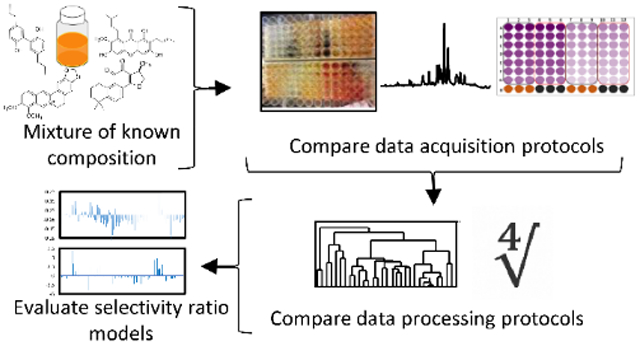
Graphical Abstract

Untargeted metabolomics is poised to make an impact in many areas of research, including studies to understand disease pathogenesis,¹ to assess food quality and authenticity,² to monitor the environmental quality of water resources,³ to identify biomarkers,^4-6 and to discover new drugs.^7-10 Mass spectrometry is a leading tool for the generation of untargeted metabolomics datasets, largely due to the applicability of this technique to provide quantitative and qualitative data on many metabolites simultaneously across a wide range of concentrations.¹¹ Mass spectrometry metabolomics yields high-dimensional datasets that offer a detailed chemical picture of the organism in question. These data can be employed in a discovery-driven approach to guide understanding of complex mixtures and enable linkage between biological effects and the chemical profile of a given organism.^12,13 However, the interpretation of mass spectrometry metabolomics datasets is complex, requires multivariate data analysis methods, and may be confounded by experimental artefacts.^14,15 There is currently lack of consistency in the field regarding methods for collecting and interpreting metabolomics datasets, and concerns have been raised as to the reproducibly of conclusions drawn from metabolomics studies.¹⁶ In light of these concerns, the work described herein was undertaken to rigorously evaluate the advantages and limitations of metabolomics approaches for one specific application – that of identifying biologically active compounds in complex natural product extracts.

Natural products such as plants, fungi, marine organisms, and bacteria have been utilized as medicines throughout history and continue to provide lead compounds effective against human diseases.^17,18 However, due to the diversity of identity and abundance of compounds produced by natural products, it remains challenging to assign bioactivity to individual components in such mixtures. The traditional solution to this problem is bioassay-guided fractionation,^19,20 in which active extracts and subsequent fractions are subjected to iterative chromatographic separations and biological evaluation until individual active compounds have been isolated. This process, despite its historical contribution to the discovery of important medicinal compounds, tends to be biased towards the most abundant, easily detectable, and/or easily isolatable compounds in a given mixture.^19,21 To overcome abundance bias, trace constituents can be isolated, but it is impractical to isolate all trace compounds given that natural products often contain hundreds or even thousands of constituents.²² In recent years, multiple different groups have sought to guide active constituent identification by integrating metabolomics data (chemical profiles) with biological activity data (biological activity profiles), enabling isolation efforts to be targeted towards active rather than abundant constituents.^9,23-25 Approaches that employ multivariate statistics to interpret combined chemical and biological datasets are broadly referred to as “biochemometrics.”

Several different data analytical approaches are used as tools in biochemometrics analyses. Due to the large number of variables compared to the number of samples analyzed, data from complex mixtures possess a high degree of collinearity. This poses a problem for ordinary multiple regression models, but partial least-squares (PLS) regression is capable of integrating aspects from both multiple regression and principal component analysis, making it a good starting point for biochemometrics analysis.²⁶ The resulting multicomponent PLS models are, however, often challenging to interpret. Several strategies have been developed for deciphering the meaning of PLS datasets.^9,23-25 Two graphical representations, the S-plot and the selectivity ratio plot, can be employed to visualize the information in PLS models and determine which components are likely to contribute to an observed biological activity.

The S-plot provides an avenue for identifying predictive components by plotting covariance and correlation of loading variables. Using an S-plot, constituents that have both high covariance and high correlation with the dependent variable in question can be identified.^9,27 S-plots have been successfully used in many studies to identify potential biomarkers for disease treatment,²⁸ to authenticate the origin of food crops,²⁹ and to identify medicinal compounds from botanical sources,^30,31 among others. However, the criterion of high covariance favors the identification of abundant compounds, while trace bioactive constituents may go undetected.³² Identifying points of interest can also become challenging due to the large number of spectral variables.⁹ The selectivity ratio plot³³ overcomes the abundance bias inherent to the S-plot by transforming the PLS components to enable quantification and ranking of each variable’s impact on the modeled response, i.e. bioactivity, independent of the abundance of the variables. The explained variance on the predictive PLS component is compared to the residual variance for each constituent to produce a selectivity ratio,³³ which is a measure of the predictive contribution of each variable to bioactivity.

In a recent study, fungal extracts were subjected to biochemometric analysis to determine which constituents were responsible for biological activity (ability to inhibit bacterial growth).⁹ Selectivity ratio plot analysis correctly identified altersetin from the fungus Alternaria sp. as the active constituent despite its low abundance, without being confounded by false positive results. In a parallel study, both the S-plot and the selectivity ratio plot were successful in identifying the major component macrosphelide A as the active constituent from Pyrenochaeta sp.⁹ A similar investigation was undertaken to identify compounds that enhanced the antibacterial efficacy of the alkaloid berberine within the botanical medicine Hydrastis canadensis.⁷ Biological activity data were combined with untargeted metabolomics data to produce selectivity ratio plots, which successfully identified known synergistic flavonoids and a new compound, 3,3′-dihydroxy-5,7,4′-trimethoxy-6,8-C-dimethylflavone, which also possessed synergistic activity.⁷ This study illustrated the applicability of selectivity ratio analysis to predict active components of complex botanical mixtures. It was possible to identify false positive results because they did not possess activity following isolation. However, without isolating every trace constituent in the mixture, the biochemometric models were unable to identify the frequency of false negative results.

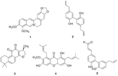
The aim of the work described herein was to evaluate the occurrence of false positive and false negative results when biochemometric analysis is conducted using selectivity ratio plot analysis and to optimize experimental conditions and data processing approaches to minimize the occurrence of both types of false results. Towards this goal, mixtures containing an inactive botanical natural product extract spiked with known antimicrobial compounds (berberine, magnolol, cryptotanshinone, and α-mangostin, compounds 1–4, respectively) were generated. Using these mixtures, the predictive power of selectivity ratio analysis was assessed in combination with several data filtering and data transformation approaches for identifying active (antimicrobial) constituents based on chemical (metabolomics) and biological data.

RESULTS AND DISCUSSION

Chromatographic Separation and Generation of Simplified Pools.

A root extract from Angelica keiskei Koidz. (Apiaceae) was chromatographically separated, and an inactive fraction was selected for use in this study. The inactive fraction was then spiked with four known constituents with antimicrobial activity (compounds 1-4) to determine if biochemometric analysis could identify the known active constituents from the complex mixture.

The spiked root extract (inactive A. keiskei fraction spiked with active compounds) was split into three chemically identical samples. Each of these samples was subjected to the same reversed-phase chromatographic separation process with each run yielding 90 test tubes. These tubes were re-combined into three pools of 30 tubes (samples 3–1 through 3–3), five pools of 18 tubes (samples 5–1 through 5–5), or ten pools of nine tubes (samples 10–1 through 10–10) to generate the simplified A. keiskei pools for biochemometric analysis and statistical comparison.

Biological Activity Assessment and Confirmation of Active Compounds.

Antimicrobial Activity Assessment.

When conducting broth microdilution assays, numerous metrics for determining bioactivity can be chosen, including percent growth inhibition, minimum inhibitory concentration (MIC) values, half maximal inhibitory concentration (IC₅₀) values, and categorical assignments of activity (i.e. active versus inactive). Each of these metrics comes with a unique set of strengths and limitations. It is well documented that in broth microdilution studies, MIC values can be placed within a three-dilution range (MIC ± 1 dilution).³⁴ Because of this, categorical assignments of samples into “active” or “inactive” categories may be less prone to misinterpretation. However, when conducting linear regression analyses (such as those completed in the PLS analyses utilized for this study), utilization of a dichotomous dependent variable (e.g. “active” and “inactive” assignments) results in a loss of information and can weaken the discriminatory pattern. As such, percent inhibition values were chosen to define the relative activities of tested samples and guide selectivity ratio analysis, as has been completed in several previous publications.^9,35

At the highest concentration tested (100 μg/mL), seven of the spiked A. keiskei pools completely inhibited the growth of Staphylococcus aureus (pools 3–1, 3–2, 5–1, 5–3, 10–1, 10–2, and 10–5). At 50 μg/mL, only four pools inhibited more than 80% of bacterial growth (pools 3–1, 3–2, 5–1, and 5–3). At 25 μg/mL, none of the treatments resulted in more than 50% inhibition. The results of these assays are summarized in Figure 1. None of the pools showed any activity at concentrations lower than 25 μg/mL (data not shown).

Figure 1.

Antimicrobial activity data of the A. keiskei root extract spiked with known antimicrobial compounds (spiked extract) and eighteen chromatographically separated pools from this original spiked extract. Pools labeled 3-1 through 3-3 represent samples resulting from chromatographic separation of the spiked A. keiskei root mixture into three pools, 5-1 through 5-5 represent samples from separation into five pools, and 10-1 through 10-10 represent samples from the ten-pool set. Growth inhibition of Staphylococcus aureus (SA1199)³⁶ is displayed as percent growth inhibition normalized to the vehicle control (broth containing bacteria but no antimicrobial compound) using OD₆₀₀ values. Data presented are the results of triplicate analyses ± SEM. Pure compounds berberine (1), magnolol (2), cryptotanshinone (3), and α-mangostin (4) served as positive controls and their minimum inhibitory concentrations (75, 6.25, 12.5, and 1.56 μg/mL, respectively), are consistent with previous reports. ^9,37-39

Quantification of Known Compounds and Predicted Activity Calculations.

Concentrations of known active compounds berberine, magnolol, cryptotanshinone, and α-mangostin (compounds 1–4) were quantified using external calibration curves (Figure S1, Supporting Information). The dose response curves of pure compounds (Figure S2, Supporting Information) were then used to predict their biological activity at 100 μg/mL. A comparison of this predicted total activity and the observed bioactivity of the relevant pool at 100 μg/mL is shown in Figure 2. Pools 3–1, 5–1, and 10–1 contained 50–75 μg/mL of berberine (compound 1), which was predicted to result in 75–100% growth inhibition. Magnolol (compound 2) was predicted to inhibit bacterial growth in the spiked extract before fractionation, as well as in pools 3–2, 5–3, and 10–5. These pools contained between 5 and 10 μg/mL of magnolol, contributing 85–100% to the predicted activity. Although fractions 10–6 and 10–7 possessed partial activity, they only contained approximately 1.5 and 0.07 μg/mL magnolol, respectively, values which are below magnolol’s activity cutoff of 3.25 μg/mL (Figure S2B, Supporting Information). Cryptotanshinone (compound 3) was predicted to inhibit 15% of bacterial growth in pool 3–2 (containing approximately 3 μg/mL) and 40% of growth in the unseparated mixture (which contained approximately 5 μg/mL). α-Mangostin (compound 4) was not present at concentrations relevant for biological activity in any of the pools tested.

Figure 2.

Predicted versus actual antimicrobial activity of A. keiskei spiked extract and pools at 100 μg/mL. Predicted antimicrobial activity was calculated by quantifying compounds 1-4 (berberine, magnolol, cryptotanshinone, and α-mangostin) in each pool and using these values to calculate predicted contribution to activity (via dose-response curves). Actual activity values represent percent growth inhibition of Staphylococcus aureus (SA1199)³⁶ normalized to the vehicle control (broth containing bacteria but no antimicrobial compound) turbidimetric OD₆₀₀ values. Data presented represent results of triplicate analyses ± SEM. Positive control data are the same as described for Figure 1.

The observed activity of six of the active pools (3–1, 3–2, 5–1, 5–3, 10–1, and 10–5) matched the predicted activity from the calculated concentration of a particular bioactive constituent in each of those pools; thus, the activity was explained almost completely by the predicted contributions of berberine and magnolol. Pools 10–2 and 10–6 demonstrated 100% and 50% activity, respectively, which could not be attributed to the predicted contributions of berberine and magnolol. Interestingly, the spiked A. keiskei mixture was predicted to completely inhibit bacterial growth, but only illustrated approximately 35% inhibition. This observation, which suggests antagonistic activity of the mixture, is discussed in detail later (see section: “Assessment of Combination Effects in Spiked A. keiskei Mixture”).

Selectivity Ratio Analysis and Comparison of Protocols.

General Findings.

PLS models for predicting active compounds were produced and visualized using selectivity ratio analysis. With these selectivity ratio models, each ion detected (represented by a m/z - retention time pair) is plotted on the x-axis, in order of m/z, and its corresponding selectivity ratio is shown on the y-axis. High selectivity ratio values represent ions that are most strongly associated with biological activity. Eighteen different models were produced utilizing samples from datasets with three different numbers of chromatographic pools (3, 5, or 10), bioactivity obtained at three different concentrations (25, 50, or 100 μg/mL), and profiles for two different pool concentrations injected into the LC-MS system (0.1 or 0.01 mg/mL). In each model, selectivity ratios were ranked from high to low, and the rankings of active compounds berberine and magnolol were evaluated. These compounds should have been identified as the top two contributors to biological activity, so better rankings are illustrated by lower numbers (with a ranking of 1 being the best). Comprehensive results of these models can be found in Table S1, Supporting Information, and a workflow can be found in Scheme 1. All peak lists, post MZMine processing, can be found in Table S2, Supporting Information, and raw data can be downloaded from the Global Natural Product Social Molecular Networking (GNPS) database (dataset MSV000083411).⁴⁰ In four datasets of the 18 generated, no cross-validated models could be produced. Three of these belonged to datasets obtained at low concentrations (0.01 mg/mL) injected to the mass spectrometer.

Scheme 1.

Workflow for untargeted metabolomics study in which an inactive A. keiskei root extract was spiked with known antimicrobial compounds. Biochemometric modeling results, and the impact of the of number of pools for chromatographic separation, concentration used for biological activity evaluation, and concentration injected into the LC-MS were evaluated. Additionally, the utility of data processing approaches, including data filtering and model simplification, were evaluated.

In datasets produced using chromatographic fractions separated into five (pools 5–1 through 5–5) or ten pools (pools 10–1 through 10–10), berberine and magnolol were the only constituents concentrated sufficiently to contribute to biological activity. In the three-pool datasets (modeled using pools 3–1 through 3–3), cryptotanshinone was concentrated enough to contribute to biological activity when the pools were tested at a concentration of 100 μg/mL. As such, all models produced were expected to identify both berberine and magnolol as bioactive, but only the three-pool datasets were expected to identify cryptotanshinone. Berberine was correctly identified among the top contributors to bioactivity (highest selectivity ratio) in 13 out of 14 models produced, eight of which identified berberine as the top contributor to biological activity. Magnolol was correctly identified as contributing the biological activity in all 14 models produced. Magnolol was identified among the top ten contributors to biological activity in only two out of 14 models and was identified among the top 20 contributors in in ten of the remaining models. Cryptotanshinone, due to its low abundance, was only concentrated sufficiently to contribute to biological activity in the three-pool set tested at 100 μg/mL. It was identified as the 19^th top contributor to biological activity of this mixture when injected into the LC-MS at 0.1 mg/mL, but was not identified in the dataset assessed at 0.01 mg/mL.

Many problems in statistical analysis of metabolomics datasets arise because the number of samples (in this case, chromatographically separated mixtures) is typically greatly outnumbered by the variables analyzed (i.e., m/z - retention time pairs).^14,16,41,42 For example, each model was built upon mass spectrometry data from 3, 5, or 10 samples run in triplicate. In each of these datasets, 870 ions or 370 ions were detected for sample sets assessed via UPLC-MS at 0.1 mg/mL and 0.01 mg/mL, respectively (see Experimental Section “Baseline Correction/MZMine Parameters” for MS criteria utilized to define candidate features). This low sample-to-variable ratio can lead to erroneous biological conclusions caused by correlation of non-active to active metabolites under analysis.^14,16,41,42 In all models produced, numerous compounds were predicted to be active that were in fact components of the inactive botanical extract. It is important to note that without isolating each of these compounds and testing them individually, it is impossible to confirm their lack of bioactivity. However, to conservatively estimate the success of selectivity ratio models, they have been identified here as false positives. These false positives were of two types: those that co-varied with spiked active compounds and those that did not. Co-varying false positives can be defined as compounds that were identified in the same pools, and with the same relative shifts in concentration, as active compounds. Non-co-varying false positives were identified as putatively active despite the fact they showed only minor variation across pools and did not share concentration shifts with active compounds. The identification of non-co-varying false positives is due to correlated noise, i.e. minor random variation in the bioassay data correlating to patterns in the concentration data.⁴³ The identification of these false positives is unlikely to have occurred due to injection errors, since mass spectral data were acquired in triplicate for each sample to ensure reproducibility. The authors highly recommend the inclusion of triplicate injections, which can aid in the identification of injection errors and limit erroneous classification of false positives. The distinction between co-varying and non-co-varying false positives is important because the aim is to utilize this bioinformatics approach to guide the isolation process. While co-varying false positives will lead to the chromatographic separation of pools that possess active compounds (albeit not the compounds predicted), non-co-varying false positives may lead to the separation of a sample that will not yield an active compound.

To visualize the distinction between co-varying and non-co-varying false positives, five compounds found within the five-pool set are compared in relation to biological activity (Figure 3). Relative peak areas (based on percentage of the abundance across all pools) are displayed for each compound. In this example, berberine and magnolol (orange and blue bars, respectively), which were intentionally spiked in to the mixture, are responsible for the biological activities in pools 5–1 and 5–3, respectively. Additional ions are detected in the mixture (components of the original inactive botanical mixture) that co-vary with these active compounds in a way that makes their contribution to activity indistinguishable from true active compounds (represented by yellow and gray bars in Figure 3). For a mixture of truly unknown composition, these ions would qualify as “false positives” and the analyst would not know if they or the actual known constituents were responsible for activity. Importantly, these co-varying false positives do not necessarily represent co-eluting compounds, which could represent in-source phenomena such as adducts, dimers, and neutral losses of active compounds. A non-co-varying compound (light blue bar), is found in all pools under analysis at approximately equal concentrations, yet is still identified as a potential contributor to biological activity.

Figure 3.

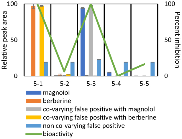
Relative peak area (expressed as a percentage of the total peak area detected across pools) of berberine (compound 1), magnolol (compound 2), and selected “false positives” identified using biochemometric modeling compared to biological activity witnessed in pools 5-1 through 5-5. Berberine and magnolol are responsible for the activity witnessed in pools 5-1 and 5-3, respectively. Co-varying false positives (yellow and gray bars) did not contribute to biological activity, but share the same abundance profiles as true active constituents across pools, and thus statistical models could not disentangle their contributions from those of the true bioactive constituents. A non-co-varying false positive (light blue bar) is also illustrated. This component does not share abundance profiles with active constituents and is found at approximately equal abundance (±5%) across all pools. It represents an example of correlated noise between the biological activity and the concentration data identified by the PLS model.

In the models produced, 2–18% of variables had selectivity ratios higher than zero, suggesting that variables in these subsets are likely to possess biological activity. Most of the false positives within these subsets were found in the same pools, and with the same relative shifts in concentration, as berberine and magnolol (representing between 43–85% of variables with selectivity ratios higher than zero across all models produced, Table S3, Supporting Information). These false positives likely do not represent in-source phenomena associated with berberine or magnolol, as the majority of their retention times are not the same as these active constituents nor do they possess the expected m/z values as common adducts (Table S2 Supporting Information). However, it is possible that a small minority of the co-varying false positives represent unexpected in-source phenomena associated with magnolol. All models produced for low concentration datasets (0.01 mg/mL) had false positives that did not co-vary with known active compounds representing between 13–43% of variables with selectivity ratios greater than zero (Table S3, Supporting Information). These findings illustrate that the low concentration datasets are more prone to overfitting and may lead to false biological interpretations.

Data Acquisition and Data Processing Parameters used to Evaluate Success of Selectivity Ratio Models.

Various types of data are collected to conduct complex metabolomics studies, particularly those involving biological activity, and each stage of data collection involves choices that may affect subsequent statistical analyses. Biological activity can be measured at a range of concentrations, and LC-MS data can be acquired using samples analyzed at different concentrations. High concentrations will allow more compounds to be detected by the mass spectrometer but may risk saturating the response of highly abundant or ionizable compounds. Low extract concentrations will be less likely to be subject to saturation, but low-abundance compounds contributing to activity may be overlooked if they are below the limit of detection for the LC-MS system. Finally, the number and chemical simplicity of chromatographic pools could also influence the metabolomics models.

An important goal of this project was to evaluate the impact of the number of pools, bioassay concentration, and concentration analyzed by the mass spectrometer on the final biochemometric results. To do this, models using different parameters were constructed and the resulting selectivity ratio rankings of berberine and magnolol were compared. Berberine and magnolol were chosen because they were the only two added compounds that were concentrated enough following chromatographic separation to contribute to biological activity in all models tested. The number of pools, bioassay concentration, and concentration analyzed by mass spectrometry were also assessed to determine their impact on the number of false positives, including false positives that co-varied with berberine, those that co-varied with magnolol, and those that did not co-vary with either active compound.

Effect of Data Acquisition Parameters on Selectivity Ratio Analysis.

The models produced were built using ranked data, and as such, they do not meet assumptions of normality.⁴⁴ Additionally, four of the 18 subsets did not produce models, leading to a breakdown of orthogonality. As such, partial least squares (PLS) analysis was chosen to assess the impact of the number of pools, bioassay concentration, and concentration injected into the LC-MS system on each of the result metrics (ranking of berberine, ranking of magnolol, false positives co-varying with berberine, false positives co-varying with magnolol, and non-co-varying false positives). The model generated to assess the variability among the selectivity ratio rankings of berberine explained 32.4% of the variability (R² = 0.324), suggesting that the number of pools included in the model, the bioassay concentration, and the mass spectral concentration have only a minor effect on the ability of selectivity ratio models to identify berberine as active. Similar results were found with selectivity ratio rankings of magnolol. Data acquisition parameters had a greater effect on the selectivity ratio rankings of magnolol than berberine (R² = 0.484). The number of pools and the concentration tested in the bioassay did not have much impact on either model produced, and most of the variability was explained by concentration injected into the LC-MS, with high concentration datasets leading to better selectivity rankings. False positives co-varying with berberine were modeled using a one-component model (R² = 0.627), and the number of false positives increased with increased concentration injected into the LC-MS. Interestingly, the false positives co-varying with magnolol were found to increase with the number of pools (R² = 0.901). Non-co-varying false positives increased with the number of pools and decreased with increasing concentration injected into the LC-MS and used in the bioassay (R² = 0.556).

Models produced using high concentrations in the LC-MS (0.1 mg/mL) were comprised of 870 unique ions. Of these 870 ions, a subset of ions, representing 2–5% of the total number of ions, had selectivity ratio rankings greater than zero. The low-concentration dataset (0.01 mg/mL) was comprised of 370 ions and a subset containing 9–18% of the total number of ions possessed selectivity ratio rankings greater than zero. In all cross-validated models, between 14–34% of variables with selectivity ratios greater than zero represented berberine or magnolol, including adducts and isotopes (Table S3, Supporting Information). These analyses revealed that datasets analyzed at higher concentrations analyzed in the LC-MS (0.1 mg/mL rather than 0.01 mg/mL) had improved selectivity ratio rankings for both berberine and magnolol, and also reduced the number of false positives that did not co-vary with active compounds (Table S1, Supporting Information). These results suggest that saturation of highly abundant compounds (such as berberine) did not result in a breakdown of linearity and allowed for the identification of active compounds. Models were made worse when assessed at lower concentrations, particularly for magnolol selectivity ratio rankings (Table S1, Supporting Information). Based on this observation, it can be inferred that low concentrations, magnolol may be present at levels near or below the limit of quantification, skewing the linearity of the response and decreasing its contribution to the model. Low-concentration datasets appeared to be more prone to identifying correlated noise, as illustrated by the increased number of non-co-varying false positives (Table S1, Supporting Information). Although there were more false positives that co-varied with berberine in the high concentration datasets, these numbers were small (one or two false positives), and as such, the benefits of high concentration analysis outweigh the risk of false positives. Not only are high-concentration datasets less likely to identify non-co-varying false positives as active, they also provide a smaller pool of putative active compounds than those of low concentration datasets (2–5% versus 9–18%, Table S3, Supporting Information).

Effect of Data Processing Approaches on Selectivity Ratio Analysis.

Because of the immense complexity of botanical extracts, it is quite challenging to determine the number of metabolites present in a given sample.^14,45 Often, metabolomics datasets contain thousands of individually detected variables, whose signal intensities vary over a very large range, and may result from the detection of experimental artefacts.^14,46,47 Data pre-treatment, filtering of chemical interferents, and model simplification tools may be critically important to enable extraction of relevant information from such datasets.^14,48 To explore this possibility in the context of natural products drug discovery, the impact of data transformation, data filtering, and model simplification, as well as their second-order interactions, were assessed using data from the ten-pool set analyzed at 100 μg/mL in both the bioassay and by the LC-MS.

To measure the effects of data processing, selectivity ratio rankings of berberine and magnolol were evaluated, as well as the occurrence of false positives, including those that co-varied with berberine and magnolol and those that did not (Table S4, Supporting Information). The six terms included in these models (data transformation, data filtering, model simplification, and second-order interactions) had excellent explanatory power in all models produced, explaining 95.2% of the variance of berberine selectivity ratio rankings, 99.6% of magnolol selectivity ratio rankings, 92.4% of false positives co-varying with berberine, 99.8% of false positives associated with magnolol, and 99.7% of the non-co-varying false positives. Depending on the combination of data processing approaches utilized, drastic changes in the selectivity ratio ranking of berberine (ranging from first to 23^rd) and magnolol (ranging from eighth to 213^th) were witnessed. A wide range was also witnessed for all categories of false positives (Figure 4, Table S4, Supporting Information). These results suggest that data processing approaches are particularly important for extracting reliable information from metabolomics datasets.

Figure 4.

Comparison of selectivity ratios produced with different data processing approaches. All models were derived from the ten-pool set analyzed at 0.1 mg/mL in the mass spectrometer using bioassay data at 25 μg/mL. m/z-retention time pairs (x-axis, low to high m/z) are plotted relative to their selectivity ratios (y-axis). The most positive bars (selectivity ratios) represent compounds with the highest ratio of explained to residual variance, and are predicted to be associated with biological activity. A series of identified features were associated with berberine and marked in yellow, including an [M]⁺ ion at m/z 336.123 and retention time (R_t) 2.96 min, an [M]⁺ ion with an m/z of 338.127 and R_t of 2.961 min (containing two ¹³C isotopes), an [M]⁺ ion at m/z 339.129 min and R_t 2.94 (containing three ¹³C isotopes), and an [M]⁺ ion at m/z 336.126 at R_t 6.355 min (R_t difference because berberine was retained on the column). Two features were identified as associated with magnolol, and are marked in green, representing the [M-H]⁻ ion at m/z 265.123 and ¹³C isotope at m/z 266.127 at an R_t of 5.756 min. Polysiloxane contaminants are marked in red. 4A. No data processing approaches were used. 4B. Model simplified using a percent variance cutoff, in which ions showing less than 1% peak area variance across samples (when compared to the most variable peak) were assigned a selectivity score of zero. 4C. Model filtered using hierarchical cluster analysis (HCA), detailed in ¹⁴ 4D. Model simplified using percent variance cutoff and filtered with HCA. 4E. Model produced using peak area data subjected to a fourth-root transformation. 4F. Model using transformed data and a percent variance cutoff. 4G. Model using transformed data and HCA filtering. 4H. Model produced with transformed data, filtered with HCA, and simplified using a percent variance cutoff. The model produced in Figure 4D has the lowest rate of false positives and the best selectivity ratios for both berberine and magnolol, illustrating that its combination of data processing techniques is most suitable for this application.

Data Transformation.

It is common practice in metabolomics studies, particularly those utilizing mass spectrometric data, to subject data to a transformation procedure.^48,49 Since mass spectrometers are so sensitive in their ability to detect compounds at a wide range of concentrations, they are subject to errors caused by heteroscedastic noise in count data, in which error is proportional to the peak area.^48,49 As such, data transformation processes aimed to reduce the error associated with large peak areas are commonly employed.^48,49 Many metabolomics projects utilize, for example, a fourth-root transformation of variable peak areas to minimize the impact of heteroscedastic noise and reduce bias against highly abundant or ionizable compounds.^9,49,50 Despite the popularity of this approach, the statistical analysis revealed that this transformation negatively impacted the ability of models to accurately predict active compounds. Models built using transformed data (Figures 4E-4H) gave berberine and magnolol worse selectivity ratio rankings than datasets using non-transformed data (Figures 4A-4D). There were also more false positives that did not co-vary with active compounds and that co-vary with berberine. Somewhat surprisingly, no false positives that co-varied with magnolol were detected in models that did not use transformed data. Likely, models that used transformed data were unable to identify magnolol as important for bioactivity, and as such, the compounds that co-varied with magnolol were not identified either. As the non-transformed datasets were able to identify magnolol as active, the false positives associated with magnolol also increased. These results are counter to the findings of other studies.⁵⁰ For example, while Arneberg et al.⁵⁰ found that the n^th root transformation positively impacted their models, models built using this transformation were unable to identify active constituents. These differences may be due to the differences in applications between these two projects. While Arneberg et al.⁵⁰ were assessing proteomics datasets, the datasets assessed for this project were focused on metabolomics-driven natural products discovery. In natural products discovery projects, low-abundant constituents that contribute to bioactivity may be present in the upper parts per million or parts per thousand range,⁵¹ while protein biomarkers are often found in the lower parts per billion range.^52,53 A transformation to reduce the impact of major peaks compared to minor peaks may be helpful when the compounds of interest are likely to be extremely low in abundance, but not necessarily in the case of natural products discovery. Another potential reason for the negative impact of transformation on selectivity ratio models is that the fourth-root transformation is a nonlinear transformation, which may cause a breakdown in the linear relationship between active compound concentration and bioactivity.

Model Simplification.

The goal of this project is to identify active constituents from complex botanical mixtures; therefore, supervised methods using biological activity as the dependent variable should be used. Since the biological activity varies from sample to sample (Figure 1), the variables responsible for biological activity should also vary in concentration from sample to sample. To reduce the influence of variables that do not vary in concentration across pools on model interpretation, peak area variance was assessed. Variables were ranked according to their overall peak area variance between pools, and the variable with the highest variance was used as a reference. If variables contained an overall peak area variance that was less than 1% than that of the reference variable, it was assigned a selectivity ratio of zero. Datasets that were evaluated using this approach (Figures 4B, 4D, 4F, and 4H) had better selectivity ratio rankings for berberine and magnolol than those that did not (Figures 4A, 4C, 4E, and 4G). Additionally, there were fewer false positives that co-varied with berberine and that did not co-vary with active compounds in simplified models when compared to their non-simplified counterparts. There were more false positives associated with magnolol in models that were produced using this simplification process, possibly because simplified models were better able to identify magnolol, and variables correlated with it, as important for biological activity.

Interaction between Data Transformation and Model Simplification.

Multiple studies have been conducted to evaluate the influence of data processing treatments on subsequent data analysis, and have revealed that there are often complex interactions between the parameters used.^50,54 To optimize data treatment parameters, it is important to inspect interactions between processing steps. Indeed, statistical analyses also revealed a strong interaction between two data processing steps: data transformation and model simplification using a percent variance cutoff (Figures 4B and 4D). Models that did not use transformed data were better than their transformed counterparts at identifying berberine and magnolol as active only when model simplification using a percent variance cutoff was utilized. Transformed datasets were barely improved using this simplification method, likely because the data transformation minimized peak area variance between different ions. Models evaluated without data transformation and with a percent variance selectivity ratio filter (Figures 4B and 4D) showed enhanced selectivity ratio rankings for both berberine and magnolol. The selectivity ratio ranking for berberine in these models was first or second, while all other models had selectivity ratio rankings between 17 and 23. The ranking of magnolol was eighth or ninth in models that were not transformed but were simplified using a percent variance selectivity ratio filter, while all other models had magnolol selectivity ratio rankings between 110 and 213. The number of false positives that did not co-vary, as well as false positives co-varying with berberine, were also reduced. Again, the number of false positives co-varying with magnolol was increased in these datasets (Table S4, Supporting Information).

Data Filtering using Relative Variance and Hierarchical Cluster Analysis of Triplicate Injections.

Often in mass spectrometry-based metabolomics, background noise and chemical contaminants are assumed to be consistent across samples. However, as illustrated in a recent study by the authors,¹⁴ this is not always the case. Chemical interferents originating from the analytical instrumentation itself,^55,56 including silica capillary contaminants and HPLC column packing materials, may be introduced differentially from injection to injection, in which case they will not be consistent across samples. Data filtering for removal of these contaminants from metabolomics datasets can improve quality and interpretability. This data filtering approach, when applied to the data collected herein, did not result in statistically significant changes to selectivity ratio rankings of berberine and magnolol, nor in the number of false positives identified (Table S4, Supporting Information). However, in all models that did not go through this data filtering process, between one and four contaminants were incorporated into the model predictions. In one example, a known polysiloxane contaminant⁵⁷ was falsely identified as the top contributor to biological activity (Figure 4B, Table S4, Supporting Information). Since many metabolomics studies rely on the assumption that compounds that vary in abundance from sample to sample may have biological importance, these types of contaminants are particularly important to identify and remove from metabolomics datasets.

Assessment of Combination Effects in Unfractionated, Spiked A. keiskei Mixture.

Many studies have shown that the observed biological activity of botanical mixtures may be due to the combined action of multiple constituents, which can interact additively, synergistically, or antagonistically.^7,58-61 For the study conducted here, it was hypothesized that such combination effects could be responsible for the large discrepancy in the predicted and observed activities for the spiked A. keiskei botanical extract (Figure 2). Specifically, it was proposed that constituents of the “inactive” botanical extract might mask or antagonize the antimicrobial activity of the antimicrobial compounds that had been spiked into it. To test this hypothesis, a checkerboard assay typically employed to assess synergy and antagonism in antimicrobial activity^7,61,62 was conducted in which purified berberine and magnolol were tested individually for antimicrobial activity in combination with a range of concentrations of the spiked A. keiskei mixture. The results of the synergy assay were illuminating, as illustrated in Table 1 and Figure 5. The spiked extract, when tested in combination with berberine, caused the minimum inhibitory concentration (MIC) of berberine to change from 75 μg/mL to 150 μg/mL and the IC₅₀ to change from 29.5 μg/mL to 85 μg/mL (Figure 5A). Although these numbers may be suggestive of an antagonistic effect, using conservative ΣFIC indices, this effect was considered “noninteractive”.⁵⁹ The spiked A. keiskei mixture had an even more notable impact on antimicrobial activity of magnolol (Figure 5B). The MIC of magnolol in combination with the spiked A. keiskei extract was increased to 25 μg/mL, when in pure form the MIC of magnolol was four times lower at 6.25 μg/mL. The IC₅₀ of magnolol was also impacted and increased from 4.1 μg/mL when pure to 8.9 μg/mL in combination with 100 μg/mL of the spiked mixture. The ΣFIC index for the magnolol/extract interaction was calculated to be 5, strongly indicating the presence of antagonists in the mixture. These results explain the mismatch in activity between the predicted and observed activity (Figure 2) and confirm the prediction that the mixture contains antagonists. Unfortunately, due to material limitations, identification and isolation of antagonists in the mixture was not pursued.

Table 1.

Minimum Inhibitory Concentrations and Half Maximal Inhibitory Concentrations for Berberine (Compound 1) and Magnolol (Compound 2) Alone and in Combination with Spiked A. keiskei Extract. The MICs of Berberine and Magnolol in Isolation are Consistent with Previous Reports.^9,37

Treatment	MIC (μg/mL)	IC50 (μg/mL)	FIC index a
berberine (1)	75	29.5	--
berberine (1) + spiked A. keiskei extract b	150	85	3
magnolol (2)	6.25	4.1	--
magnolol (2) + spiked A. keiskei extract b	25	8.9	5
spiked A. keiskei extract	>100 μg/mL	>100 μg/mL	--

^aΣFICs were calculated using the following equation: ΣFIC = FIC_A + FIC_B = ([A]/ MIC_A) + ([B]/MIC_B), where A and B are the compounds/extracts tested in combination, MIC_A is the minimum inhibitory concentration of A alone, MIC_B is the minimum inhibitory concentration of B alone, [A] is the MIC of A in the presence of B, and [B] is the MIC of B in the presence of A.

^bvalues expressed for magnolol and berberine’s MIC/IC₅₀ in combination with 100 μg/mL spiked extract.

Figure 5.

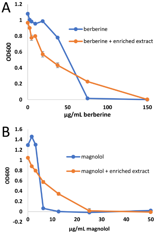
Comparison of dose-response curves for berberine (compound 1) alone and in combination with 100 μg/mL spiked extract (A) and for magnolol (compound 2) alone and in combination with 100 μg/mL spiked extract (B). As indicated by the data shown above and the ΣFIC values in Table 1, the spiked extract antagonized the antimicrobial activity of the pure compounds. MIC values of compounds alone are consistent with previous reports.^9,37

Assessing Stage of Fractionation and Impact on Assignment of Bioactive Constituents.

Multiple Rounds of Fractionation Improve Selectivity Ratio Ranking of Magnolol.

The analyses conducted revealed that many compounds that co-varied with magnolol were incorrectly assigned as being bioactive, suggesting that another round of fractionation and biochemometrics modeling would improve the selectivity ratio ranking of magnolol and eliminate some of these false positives. To this end, three pools rich in magnolol (3–2, 5–3, and 10–5) were separated with a second stage of chromatographic separation and evaluated for their antimicrobial activity (Figure S3, Supporting Information). The chromatographic separation of pool 3–2 yielded 11 sub-pools, pool 5–3 yielded ten new sub-pools, and pool 10–5 yielded seven new sub-pools. At 50 μg/mL, four of the new sub-pools caused complete inhibition of S. aureus (SA1199)³⁶ growth (Figure S3, Supporting Information), while at 25 μg/mL, the most active sub-pool exhibited 60% inhibition.

Six new selectivity ratio models (two from each of the three new sets of sub-pools, assessed at 25 and 50 μg/mL) were produced using the sub-pool data from the second-stage fractionation (Figure S4, Supporting Information), and these models were compared with the models generated from the previous round of fractionation (Table S5, Supporting Information). The second-stage models had significantly higher selectivity ratio rankings for magnolol. Five of the six second stage models ranked magnolol between the 1^st and 6^th top contributors to biological activity (median ranking = 2), while their first stage counterparts ranked between fourth and 14^th (median ranking = 13). Contrary to the predictions made, the number of false positives was not affected by an additional round of fractionation.

Although the number of false positives found in the same chromatographic pools as magnolol were not affected, magnolol’s contribution to the overall selectivity ratio models is more notable with second-stage pools. As an example, first- and second-stage selectivity ratio models for the ten-pool set, analyzed at 0.1 mg/mL in the mass spectrometer, and assessed at 25 μg/mL are compared in Figure 6. Only the top 20 predicted contributors to biological activity are color coded. In this figure, red bars represent variables that co-varied with magnolol that were falsely identified among the top contributors to biological activity. Green bars represent magnolol and its associated masses (i.e., ¹³C-isotopes). Blue bars are false positives that co-varied with berberine, and purple bars represent non-co-varying false positives. In Figure 6A, berberine and associated masses (yellow bars) are easily identifiable as putative active compounds, as are additional compounds that represent both co-varying and non-co-varying false positives. The green bars associated with magnolol are identified among the top 20 contributors to biological activity, but their relative magnitude is considerably smaller than many false positives. In Figure 6B the only false positives identified co-varied with magnolol, and magnolol’s relative contribution to the model is improved. Berberine was not identified in this model because it was not present in the pools selected for sub-fractionation.

Figure 6.

Models produced using pools 10-1 through 10-10 (6A) and 10-5-1 through 10-5-7 (6B) analyzed at 0.1 mg/mL in the mass spectrometer, and assessed for activity at 25 μg/mL. Features associated with berberine (compound 1) are marked in yellow, and represent an [M]⁺ ion at m/z 336.123 and retention time (R_t) 2.96 min, an [M]⁺ ion with an m/z of 338.127 and R_t of 2.961 min (containing two ¹³C isotopes), an [M]⁺ ion at m/z 339.129 min and R_t 2.94 (containing three ¹³C isotopes), and an [M]⁺ ion at m/z 336.126 at R_t 6.355 min (R_t difference due to column retention). Features associated with magnolol (compound 2) are marked in green. In both 6A and 6B bars represent the [M-H]⁻ ion at m/z 265.123 and ¹³C isotope at m/z 266.127 at an R_t of 5.756 min. Two additional associated ions, the [M-H]⁻ ion at m/z 265.124 with an R_t of 5.72, and the [M-H]⁻ ion containing 2 ¹³C isotopes at m/z 267.129 with an R_t of 5.73 are found in 6B. Co-varying false positives can be defined as compounds that were identified in the same pools, and with the same relative shifts in concentration, as active compounds. Non-co-varying false positives, on the other hand, were identified as putatively active but did not share concentration patterns with active compounds. In this figure, red bars correspond to variables co-varying with magnolol, blue bars represent false positives co-varying with berberine, and purple bars represent non-co-varying false positives.

Although false positives still prevailed in the model predictions after additional rounds of fractionation, it is important to note that all the false positives in the top 20 contributors to activity in the second-stage model (Figure 6B) represent co-varying false positives. Since the impact of non-co-varying false positives was minimized by sub-fractionation, prioritization of pools for future chromatographic separation is more straightforward. Likely, an additional round of fractionation and modeling would improve this even further. These results are consistent with a recent study conducted exploring the use of biochemometrics and its ability to identify synergists in Hydrastis canadensis.⁷ With this project, three rounds of fractionation were required to produce a reliable selectivity ratio model. This model successfully identified known synergists in H. canadensis and revealed the activity of a previously undescribed compound.⁷ In another study using biochemometrics and molecular networking to identify important constituents from A. keiskei, two rounds of fractionation data were required before antimicrobial compounds were identified.³⁵ Thus, it appears that, as would be expected, biochemometric model predictions improve upon chromatographic separation. With the first set of models produced using complex first-stage pools, berberine was consistently identified among the top contributors to biological activity while magnolol was not. The pool containing the highest abundance of berberine from the first stage of chromatographic separation contained only 212 variables above the baseline, while the pool containing magnolol contained nearly twice as many compounds. However, after a second round of fractionation, the sub-pool containing the highest amount of magnolol only showed 310 ions above the baseline, making statistical modeling more efficient and less prone to data overfitting (Figure S5, Supporting Information).

Multiple Rounds of Fractionation Revealed an Additional Bioactive Constituent Previously Masked by Antagonists in the Mixture.

For the data shown in Figure S3, Supporting Information, the activity can be attributed to magnolol in sub-pools 3–2-11, 5–3-7, and 10–5-5, where magnolol was present at concentrations higher than its MIC (6.25 μg/mL) in sub-pools tested at 50 μg/mL (7.5 ± 1.2, 9.2 ± 0.4, and 10.5 ± 0.3 μg/mL for sub-pools 3–2-11, 5–3-7, and 10–5-5, respectively). However, sub-pool 10–5-2, which also inhibited growth of S. aureus (SA1199)³⁶ at 50 μg/mL, did not contain detectable levels of magnolol. Rather, this sub-pool was comprised almost entirely of another compound (93% purity based on LC-UV analysis, data not shown). This pool was subjected to an additional round of chromatographic separation, yielding randainal (5, 0.25 mg, 99% purity). Due to the structural similarity of randainal to magnolol, this compound likely did not originate from the A. keiskei root extract, but rather represented an oxidation product of magnolol. Indeed, randainal was not detected in the unspiked A. keiskei extract used for these studies (data not shown).

Randainal was predicted by one second-stage model to be the fifth top contributor to biological activity. Nine false positives co-varied with randainal, and six false positives co-varied with magnolol. Three additional false positives were identified that did not co-vary with either of the active constituents. The discovery of randainal was illuminating and highlights the importance of fractionation for identifying low-abundance antimicrobials that may be masked by combination effects. It appears that the presence of antagonists in the A. keiskei roots (Figure 5, Table 1) masked the biological activity of randainal until it had been chromatographically separated from them. Although purified randainal was not tested for activity due to material limitations, its structural similarity to magnolol suggests that compounds present in the original A. keiskei mixture antagonized its activity in a similar way. Sub-pool 10–5-2 (93% randainal) was found to be active at 50 but not 25 μg/mL, which is likely the range of activity for randainal, although it is possible that minor constituents in the mixture also contributed.

The discovery of randainal also provided additional insight into models from the first round of data collection. Pool 10–6 possessed partial activity that was not explained by the four active compounds that were spiked into the mixture; however, this pool contained randainal, which likely contributed to the activity witnessed. Additionally, five of the original models identified randainal among the top contributors to biological activity (Table S6, Supporting Information). These masses were originally thought to be false positives that co-varied with magnolol.

Limitations and Opportunities.

Mass spectrometry is the analytical technology of choice in the metabolomics field because of its sensitivity to structurally diverse chemicals at a wide range of concentrations and ionization efficiencies. While mass spectrometry provides complex chemical profiles with the ability to reveal valuable scientific insights into various biological processes, it also is fraught with challenges. Especially when exploring complex biological organisms for unknown compounds, the analyst must contend with the fact that many variables detected may not represent compounds associated with the sample. Additionally, differences in ionization efficiencies of analytes detected can have major impacts on the statistical models produced. For example, it was found that models produced when injecting higher concentrations into the mass spectrometer (0.1 mg/mL) were generally more informative than those assessed at low concentrations (0.01 mg/mL). Although these models were at a higher risk for saturating the response of highly abundant compounds, they provided a more complete picture of true sample components. The low concentration datasets likely resulted in models that were skewed by highly abundant compounds, highly ionizable compounds, and noise. Low-concentration models were less useful for identifying active compounds and were also more prone to the inclusion of non-co-varying false positives due to correlated noise. Interestingly, data acquisition factors tended to impact the ranking of compounds identified as contributing to biological activity, but the identity of these candidates was relatively consistent.

Metabolomics datasets rely not only on the data acquired, but also upon the data pre-treatment and data processing steps utilized. Unlike data acquisition parameters, which affected the order but not identity of the top 50 ions produced, data processing parameters had a drastic impact on both the order and identity of predicted bioactive constituents. Using a factorial design, the effects of data filtering, data transformation, and model simplification steps on selectivity ratio analysis were evaluated, and it was found that most of these models produced were unable to identify known active constituents and contained many putatively false relationships. One of the most substantial findings of this work was that data transformation, though commonly employed in metabolomics studies,^48,49 had a negative impact on subsequent statistical analyses. These results suggest that data-processing protocols should be chosen carefully based on the goals of the project at hand and that commonly employed tools for one application may be unnecessary, or even detrimental, for other applications. It was discovered that not only are individual pretreatment and processing steps influential (particularly model simplification using a percent variance cutoff and data transformation), but their interactions also have major impacts on models produced. Finally, strategies to remove ions that do not represent real sample components are important for understanding the chemistry of the sample under analysis. Datasets that were not filtered using protocols described in a recent publication¹⁴ contained false positive peaks associated with LC-MS equipment used for analysis. These peaks were often putatively identified as the top contributors to biological activity when the filtering approach was not utilized.

Even if all data acquisition and data processing parameters are optimized, there will likely be false negatives that are not incorporated into the model and false positives that are. For this experiment, four active compounds were spiked into a complex mixture. However, only two of these active compounds were concentrated enough to show biological activity. α-Mangostin, notably, was the most potent antimicrobial compound that was utilized; however, its low concentration in the pools that resulted from chromatographic separation prevented it from being detected as an active component of the original mixture. Cryptotanshinone was identified only in some of the models in which it was present at biologically relevant concentrations. Multiple rounds of fractionation may serve to concentrate low abundant active compounds enough to reveal their activity.

It is worth mentioning that the possibility of missing highly active compounds when they are present at low concentration is not only an inherent limitation of the biochemometric approach employed here, but of any bioassay-guided fractionation experiment. It is almost always true that the analytical approach employed to profile natural product extracts and pools will be more sensitive than the biological assay employed to evaluate their activity. Thus, it is always possible for a detected compound to be falsely deemed “inactive” simply because it is present at levels too low to register a biological effect.

False positives are also a problem in biologically driven metabolomics analysis. There will always be compounds that happen to be present in the same pools and at the same relative concentrations as true active constituents, so it is no surprise that inactive compounds may be predicted to be active using a biochemometric approach. By utilizing optimized parameters for data processing and acquisition, it is possible to influence the type of false positives included in the model. False positives that are found in pools associated with biologically active constituents are less problematic than those that are not, because the fractionation process is guided by the predictions of the model. It was also found that antagonism can mask the activity of active compounds and distort metabolomics models. An additional round of fractionation allowed not only for the improved identification of magnolol as active, but it also revealed an additional active compound, randainal, which was masked by combination effects. This compound was previously believed to be a false positive that was simply found in the same pools as magnolol. This finding suggests that many of the “false positives” that were counted in this study may not truly be false positives at all but may represent active compounds with activities that have been distorted by combination effects.

Untargeted metabolomics is a tool for finding a needle in a haystack. For natural products drug discovery, the goal is often to identify bioactive “needles” in a haystack of thousands of metabolites. The studies described herein demonstrate that biochemometric approaches cannot necessarily identify the needle from the entire haystack, but rather, they can be applied to reduce the large haystack to a much smaller one that is likely to contain active compounds. Selectivity ratio analysis is an excellent tool to rank lead compounds in this smaller haystack and prioritize them for isolation. Effort is still required to purify the putative active compounds, assign their structures, and test them for biological activity. The studies presented herein demonstrate that such validation is very necessary, given the likelihood of identifying false positives. However, the finite quantity of material available for subsequent isolation poses an inherent limitation that often stymies such validation.

CONCLUSIONS

The vast, largely unknown chemical landscape of botanicals is deeply rich, and although tools to understand the nature of their bioactive properties are improving, it is important to recognize that multivariate models are affected by a variety of biological, chemical, and analytical factors. Biochemometric approaches can be used to unveil valuable insights that otherwise remain hidden. However, extracting information out of these large datasets remains challenging. Despite this, researchers should not allow themselves to be stagnated by imperfect or incomplete interpretations; rather, the incomplete knowledge should be used to generate hypotheses and improve interpretation and methods over time. This reality brings to mind statistician John Tukey’s statement: “Far better an approximate answer to the right question . . . than an exact answer to the wrong question. Data analysis must progress by approximate answers, at best, since knowledge of what the problem really is will at best be approximate.”⁶³ Although Big Data approaches may not find the exact answer to the question at hand, the effective management of large datasets gives researchers the ability to find better questions, recognize limitations, and follow up on predictions in an informed way.

EXPERIMENTAL SECTION

General Experimental Procedures.

UPLC-MS analysis was conducted in both the positive and negative modes using a Thermo-Fisher Q-Exactive Plus Orbitrap mass spectrometer (Thermo Fisher Scientific, MA, USA) connected to an Acquity UPLC system (Waters Corporation, Milford, MA, USA). UPLC-MS analyses were completed using a reversed-phase UPLC column (BEH C₁₈, 1.7 μm, 2.1 × 50 mm, Waters Corporation, Milford, MA, USA). Each sample was analyzed in triplicate at concentrations of 0.1 mg/mL and 0.01 mg/mL in methanol (expressed as mass of sample per volume of solvent) with a 3 μL injection. Chromatographic separation was accomplished using a gradient comprised of water with 0.1% formic acid (solvent A) and acetonitrile with 0.1% formic acid (solvent B). The starting conditions were 90:10 (A:B) and held for 0.5 min. Over 0.5–8.0 min, the gradient was increased to 0:100 (A:B) and held at these conditions until 8.5 min. Over the next 0.5 min, starting conditions were re-established, and the gradient was held at 90:10 (A:B) from 9.0–10.0 min. Mass analysis (in both the positive and negative modes) was completed over a m/z range of 150–1500. The settings were set as follows: capillary voltage −0.7 V, capillary temperature 310°C, S-lens RF level 80.00, spray voltage 3.7 kV, sheath gas flow 50.15, and auxiliary gas flow 15.16. A data-dependent method was used, and the four ions with the highest signal intensity were fragmented with HCD of 35.0.

Production of Spiked Botanical Mixture with Known Antimicrobial Compounds.

The goal of this project was to evaluate the effectiveness of selectivity ratio analysis to identify known active (antimicrobial) compounds in an otherwise inactive mixture. Detailed information about the plant material, extraction, and simplification of this mixture can be found in the Supporting Information. To prepare the spiked extract, a simplified and inactive Angelica keiskei Koidzumi extract (126.4 mg) was combined with four known antimicrobial compounds at different concentrations yielding 167.9 mg of the spiked extract: berberine chloride (1, 24.9 mg, 15% of extract mass), magnolol (2, 11.6 mg, 7% of extract mass), cryptotanshinone (3, 3.3 mg, 2% of extract mass), and α-mangostin (4, 1.7 mg, 1% of extract mass). This resulting mixture, containing both unknown compounds and known active compounds, was used as the test material for the experiments described herein.

Chromatographic Separation Experiments.

The spiked A. keiskei root mixture was separated into three equal portions and reversed-phase HPLC was conducted. Each separation was conducted using the same gradient and column (Gemini NX reversed-phase preparative HPLC column, 5 μm C₁₈, 240 × 21.20 mm; Phenomenex, Torrance, CA, USA) with a flow rate of 21.4 mL/min. The gradient began with 30:70 CH₃CN-H₂O, after which it was increased to a ratio of 55:24 over 8 min. The gradient was then increased to 75:25 over two min and ramped up to 100% CH₃CN for 28 min. The 100% organic gradient was then held for another two min to flush the column.

Each fractionation yielded 90 test tubes, which were divided evenly into sets containing three, five, or ten pools, facilitating assessment of the impact of chromatography and pool complexity on biochemometric analysis. The first set of pools consisted of three pools of 30 tubes each (pools 3–1 through 3–3), the second set was made up of five pools with 18 tubes each (pools 5–1 through 5–5), and the final set was ten pools of nine tubes each (pools 10–1 through 10–10). Each pool was dried under nitrogen before subsequent analysis. The complete fractionation scheme is provided as Figure S4, Supporting Information.

Following the first round of biochemometric analysis, three pools were selected for a second round of chromatographic separation. The magnolol-rich pools (pools 3–2, 5–3, and 10–5) were subjected to another round of reversed-phase HPLC. All pools were separated using a gradient comprised of acetonitrile and water through a Gemini NX reversed-phase preparative HPLC column (5 μm C₁₈, 240 × 21.20 mm; Phenomenex, Torrance, CA, USA) with a flow rate of 21.4 mL/min. Pool 3–2 was separated using a gradient beginning with 45:55 CH₃CN-H₂O and increasing to 60:40 CH₃CN-H₂O over 30 min after which it was flushed with 100% acetonitrile for 10 min. Pool 5–3 was separated into ten sub-pools using a gradient increasing from 60:40 to 70:30 CH₃CN-H₂O over 25 min and ending with a 10 min flush of 100% acetonitrile. Finally, pool 10–5 was separated into seven sub-pools (10–5-1 through 10–5-7) with an isocratic gradient of 60:40 CH₃CN-H₂O held for 30 min before a 10 min flush of 100% acetonitrile. Sub-pool 10–5-2, collected from 9–10 min, was subjected to a final round of reversed-phase HPLC through a Phenomenex Gemini-NX reversed-phase analytical column (5 μm; 250 × 4.6 mm) with a 35 min gradient of CH₃CN-H₂O starting at 30:70 and increasing to 70:30 following which it was increased to 100:0 for 5 min. Randainal (5)^64,65 was collected from 20–20.5 min (0.25 mg, 99% purity). NMR spectra were collected using an Agilent 700 MHz spectrometer (Agilent Technology) or a JEOL ECA-500 MHz spectrometer (JEOL, Peabody, MA, USA).

Randainal (5): yellow, amorphous powder; HRESIMS m/z 279.1028 [M-H]⁻ (calculated for C₁₈H₁₅O₃⁻, 279.1021). Fragmentation patterns matched predicted patterns as well as previously reported fragments from the literature⁶⁴ (Figure S6, Supporting Information). ¹H NMR data, HSQC data, and HMBC data (700 MHz, CD₃OD) are provided as Figures S7-S9 in Supporting Information. Previous literature reports on this compound were completed in acetone-d₆ ⁶⁵. To confirm the identity of this compound, an additional ¹H NMR was run (500 MHz, acetone-d₆), and chemical shifts matched literature values (Figure S10, Supporting Information).⁶⁵

Antimicrobial Assay.

To assess antimicrobial activity, a broth microdilution assay was completed for each pool using a laboratory strain of Staphylococcus aureus (SA1199).³⁶ Assays were conducted using Clinical Laboratory Standards Institute (CLSI) standard protocols.⁶⁶ Cultures were grown in Müeller-Hinton broth (MHB) from an isolated colony and diluted to 1.0 × 10⁵ CFU/mL calculated using absorbance at 600 nm (OD₆₀₀) values.

As one of the goals for this project was to assess the impact of bioassay data format on biochemometric results, a full dose-response curve was collected for each pool and each known antimicrobial compound. Stock solutions were prepared in DMSO and diluted with MHB so that final concentrations in test wells would contain 2% DMSO. Using these stock solutions, samples were screened in triplicate at concentrations ranging from 0–100 μg/mL in MHB (or 0–150 μg/mL in the case of berberine). The 28 sub-pools produced during the second round of fractionation were screened for bioactivity testing at two concentrations: 50 and 25 μg/mL. Chloramphenicol was used as a positive control. Each well was inoculated with bacteria (at 1.0 × 10⁵ CFU/mL) and incubated for 18 h at 37 °C. After incubation, OD₆₀₀ was calculated using a Synergy H1 microplate reader (Biotek, Winooski, VT, USA) and used to calculate the growth inhibition of Staphylococcus aureus by the pools and/or compounds tested. Minimal inhibitory concentrations (MICs) were calculated for each of the known compounds, defined as the concentration at which there was no statistically significant difference in OD₆₀₀ values between the negative control (wells containing broth and samples but no bacteria) and the treated sample. Dose-response curves were produced using a four-parameter logistic model in SigmaPlot (v.13, Systat Software, San Jose, CA, USA).

Synergy Assessment.

Antimicrobial checkerboard assays using a broth microdilution method^61,62 were conducted to assess the effect of the spiked extract on the antimicrobial efficacy of berberine and magnolol. The A. keiskei extract, spiked with berberine, magnolol, cryptotanshinone, and α-mangostin, was tested in combination with berberine or magnolol, with the spiked A. keiskei extract and magnolol ranging in concentration from 1.56–100 μg/mL, and berberine ranging from 2.34–150 μg/mL. The vehicle control was comprised of 2% DMSO in Müeller-Hinton broth. The fractional inhibitory concentration index (ΣFIC) for each combination of compounds was calculated using equation 1:⁶¹

$$\begin{gathered} \Sigma \mathrm{FIC}=FI{C}_A+FI{C}_B \\ \text{Where}FI{C}_A=\frac{[A]}{MI{C}_A},\mathrm{and}FI{C}_B=\frac{[B]}{MI{C}_B} \end{gathered}$$ (equation 1)

A and B are the compounds/extracts tested in combination, MIC_A is the minimum inhibitory concentration of A alone, MIC_B is the minimum inhibitory concentration of B alone, [A] is the MIC of A in the presence of B, and [B] is the MIC of B in the presence of A. To minimize the risk of misinterpretation of data, which is common in interaction studies,^59,67-72 conservative values were chosen to assign combination effects as recommended in the review by van Vuuren and Viljoen.⁵⁹ For the purposes of this project, synergistic effects are defined as interactions having an ΣFIC ≤ 0.5, additive effects have an ΣFIC between 0.5 and 1.0, non-interactive effects have ΣFIC values between 1.0 and 4.0, and antagonistic effects have ΣFIC values ≥ 4.0.

Quantitative Analysis of Known Compounds and Contribution to Biological Activity.

Concentrations of the known active compounds berberine, magnolol, cryptotanshinone, and α-mangostin were determined in the chromatographically separated fractions using LC-MS. An external calibration curve of each standard compound (with final concentrations ranging from 0–50 μg/mL in methanol) was produced to identify the linear range of the calibration curve. Each sample was re-suspended in methanol to a concentration of 0.1 mg/mL and analyzed as described in the “General Experimental Procedures.” Subsequent concentrations were calculated from the relevant calibration curve based on the peak area of the relevant selected-ion chromatogram for each compound in each sample. Antimicrobial dose-response curves of each compound tested in isolation were used to determine which pools possessed biologically relevant concentrations.

Statistical Analysis.

Baseline Correction/MZMine Parameters.

LC-MS datasets acquired in both positive and negative modes were individually analyzed, aligned, and filtered using MZMine 2.21.2 software (http://mzmine.sourceforge.net/).⁷³ Raw data files (including triplicate analyses of each sample) were uploaded into MZMine for peak picking. Chromatograms were built for all m/z values having peaks lasting longer than 0.1 min. The spiked extract was subjected to two stages of fractionation (Figure S4, Supporting Information). The first-stage models were produced using pools 3–1 through 10–10. Sub-pools used to produce second-stage models were generated by sub-fractionating pools 3–2, 5–3 and 10–5, and are labeled 3–2-1 through 10–5-7. Modeling completed with the first set of pools were produced using the following peak detection parameters: noise level (absolute value) of 2.0 × 10⁶ (positive mode, 0.1 mg mL⁻¹ samples), 1.0 × 10⁷ (positive mode, 0.01 mg mL⁻¹ samples), and 1.0 × 10⁶ (negative mode, both 0.1 mg mL⁻¹ and 0.01 mg mL⁻¹ samples). Models produced using the second set of pools (3–2-1 through 10–5-7) resulting from chromatographically separating magnolol-rich pools (pools 3–2, 5–3, and 10–5) were assessed at 0.1 mg/mL. For these data, the noise level was set to 2.0 × 10⁶ for both positive and negative modes. For all modeling datasets, the m/z tolerance was set to 0.0001 Da or 5 ppm, and the intensity variation tolerance was set to 20%. Peaks were aligned if they were both within 5 ppm m/z from one another and eluted within a 0.2-min retention time window. Data consisting of m/z, retention time, and peak area, for both negative and positive ions was imported into Excel (Microsoft, Redmond, WA, USA) and combined as a single peak list (Table S2, Supporting Information). Biological data were added as percent inhibition of bacterial growth at 25, 50 and 100 μg/mL. Data matrices for each sample subset (containing different pool numbers, mass spectral concentrations, and biological activity data) were independently imported into Sirius version 10.0 (Pattern Recognition Systems AS, Bergen, Norway)⁷⁴ for statistical analysis.

Hierarchical Cluster Analysis and Chromatogram Visualization.

Hierarchical clustering analysis was conducted on each data subset using Sirius version 10.0 (Pattern Recognition Systems AS, Bergen, Norway).^33,74 Briefly, samples were analyzed using an average-linkage algorithm⁷⁵ to cluster objects based on chemical similarity. A dataset was considered clustered effectively only when triplicate injections of the same sample were linked to one another before being linked to other samples. If triplicates did not show this expected trend, spectral variables were inspected for each set of triplicates. Variables showing high peak area variability within triplicate injections, as well as their associated isotopes, in-source fragments, and clusters, were removed. Datasets were also produced that did not include this filtering process to assess the importance of this process on subsequent selectivity ratio analysis. For a more detailed description of this approach, see ¹⁴.

Selectivity Ratio Analysis.

Selectivity ratios were generated with Sirius version 10.0 statistical software (Pattern Recognition Systems AS, Bergen, Norway).^33,74 As part of the goals of this project, the impacts of various data transformation and filtering approaches on the resulting biochemometric analysis were assessed. Before analysis, peak area data were transformed using a fourth-root transformation to reduce heteroscedastic noise.⁴⁹ Additional data subsets were produced in which the data were not transformed. Each subset was subjected to internally cross-validated PLS analysis using 100 iterations and a significance level of 0.05. Algorithms internal to the Sirius statistical software were computed, resulting in selectivity ratio plots that identified candidate compounds associated with biological activity. As a final filtering step, each variable within each dataset was assessed, and those showing lower than 1% peak area variance across samples were assigned a selectivity ratio of zero in order to reduce the effect of correlated noise from the datasets. This resulted in more simplified selectivity ratio plots which were compared to plots that did not include this filtering step.

Statistical Comparison of Protocols.

Partial least squares regression followed by target projection³³ and calculation of selectivity ratios²⁴ was used for calculating all models predicting biological activity from mass spectral profiles. Double cross validation³⁹ was used to determine the number of PLS components for each model.

For assessing the impact of data acquisition protocols (pool number, bioassay concentration, and mass spectral concentration) on the ranking of the bioactive candidates, PLS regression was performed with these variables and their interactions as explanatory variables in models predicting ranking of berberine and magnolol, and the number of false positives identified in the models. Similarly, the effects of fourth root transformation, data filtering, 1% variance cutoff and their two-factor interactions on the ability to reveal and rank bioactive compounds in the mass spectral data was assessed by calculating regression models with these variables and their interactions as explanatory variables.

REFERENCES

- (1).Li X; Zhang A; Sun H; Liu Z; Zhang T; Qiu S; Liu L; Wang X Oncotarget. 2017, 8(39), 65022–65041. [DOI] [PMC free article] [PubMed] [Google Scholar]
- (2).Wishart DS Trends Food Sci. Technol 2008, 19(9), 482–493. [Google Scholar]
- (3).Altenburger R; Ait-Aissa S; Antczak P; Backhaus T; Barceló D; Seiler T-B; Brion F; Busch W; Chipman K; de Alda ML; de Aragão Umbuzeiro G; Escher BI; Falciani F; Faust M; Focks A; Hilscherova K; Hollender J; Hollert H; Jäger F; Jahnke A; Kortenkamp A; Krauss M; Lemkine GF; Munthe J; Neumann S; Schymanski EL; Scrimshaw M; Segner H; Slobodnik J; Smedes F; Kughathas S; Teodorovic I; Tindall AJ; Tollefsen KE; Walz K-H; Williams TD; Van den Brink PJ; van Gils J; Vrana B; Zhang X; Brack W Sci. Total Environ 2015, 512–513, 540–551. [DOI] [PubMed] [Google Scholar]
- (4).Ackermann BL; Hale JE; Duffin KL Curr. Drug. Metab 2006, 7(5), 525–39. [DOI] [PubMed] [Google Scholar]
- (5).Sreekumar A; Poisson LM; Rajendiran TM; Khan AP; Cao Q; Yu J; Laxman B; Mehra R; Lonigro RJ; Li Y; Nyati MK; Ahsan A; Kalyana-Sundaram S; Han B; Cao X; Byun J; Omenn GS; Ghosh D; Pennathur S; Alexander DC; Berger A; Shuster JR; Wei JT; Varambally S; Beecher C; Chinnaiyan AM Nature. 2009, 457(7231), 910–4. [DOI] [PMC free article] [PubMed] [Google Scholar] [Research Misconduct Found]
- (6).van der Greef J; Hankemeier T; McBurney RN Pharmacogenomics. 2006, 7(7), 1087–94. [DOI] [PubMed] [Google Scholar]
- (7).Britton ER; Kellogg JJ; Kvalheim OM; Cech NB J. Nat. Prod 2017. [DOI] [PMC free article] [PubMed] [Google Scholar]
- (8).Chau F-T; Chan H-Y; Cheung C-Y; Xu C-J; Liang Y; Kvalheim OM Anal. Chem 2009, 81(17), 7217–7225. [DOI] [PubMed] [Google Scholar]
- (9).Kellogg JJ; Todd DA; Egan JM; Raja HA; Oberlies NH; Kvalheim OM; Cech NB J. Nat. Prod 2016, 79(2), 376–386. [DOI] [PMC free article] [PubMed] [Google Scholar]
- (10).Matsuda F Mass Spectrom. (Tokyo) 2016, 5(2), S0052. [DOI] [PMC free article] [PubMed] [Google Scholar]
- (11).Boccard J; Veuthey JL; Rudaz S J. Sep. Sci 2010, 33(3), 290–304. [DOI] [PubMed] [Google Scholar]
- (12).Efferth T; Koch E Curr. Drug Targets 2011, 12(1), 122–32. [DOI] [PubMed] [Google Scholar]
- (13).Heinrich M Phytochem. Lett 2008, 1(1), 1–5. [Google Scholar]
- (14).Caesar LK; Kvalheim OM; Cech NB Anal. Chim. Acta 2018, 1021, 69–77. [DOI] [PMC free article] [PubMed] [Google Scholar]
- (15).Yuliana ND; Khatib A; Choi YH; Verpoorte R Phytother. Res 2011, 25(2), 157–69. [DOI] [PubMed] [Google Scholar]
- (16).Marshall DD; Powers R Prog. Nucl. Magn. Reson. Spectrosc 2017, 100, 1–16. [DOI] [PMC free article] [PubMed] [Google Scholar]
- (17).Newman DJ; Cragg GM J. Nat. Prod 2016, 79(3), 629–61. [DOI] [PubMed] [Google Scholar]
- (18).Roemer T; Xu D; Singh SB; Parish CA; Harris G; Wang H; Davies JE; Bills GF Chem. Biol 2011, 18(2), 148–64. [DOI] [PubMed] [Google Scholar]
- (19).Kinghorn AD Curr. Org. Chem 1998, 2(6), 597–612. [Google Scholar]
- (20).Sharma SB; Gupta R Mini Rev. Med. Chem 2015, 15(1), 52–7. [DOI] [PubMed] [Google Scholar]
- (21).Inui T; Wang Y; Pro SM; Franzblau SG; Pauli GF Fitoterapia. 2012, 83(7), 1218–25. [DOI] [PMC free article] [PubMed] [Google Scholar]
- (22).Enke CG; Nagels LJ Anal. Chem 2011, 83(7), 2539–46. [DOI] [PubMed] [Google Scholar]
- (23).Okada T; Afendi FM; Katoh A; Hirai A; Kanaya S In Biotechnology for Medicinal Plants; Chandra S; Lata H; Varma A, Eds.; Springer: Berlin, 2013; pp 413–438. [Google Scholar]
- (24).Rajalahti T; Arneberg R; Kroksveen AC; Berle M; Myhr K-M; Kvalheim OM Anal. Chem 2009, 81(7), 2581–2590. [DOI] [PubMed] [Google Scholar]
- (25).Rajalahti T; Kvalheim OM Int. J. Pharm 2011, 417(1–2), 280–290. [DOI] [PubMed] [Google Scholar]
- (26).Abdi H In The SAGE Encyclopedia of Social Science Research Methods; Lewis-Beck MS; Bryman A; Liao TF, Eds.; SAGE Publications, Inc.: Thousand Oaks, CA, 2004; pp. 792–795. [Google Scholar]
- (27).Wiklund S; Johansson E; Sjostrom L; Mellerowicz EJ; Edlund U; Shockcor JP; Gottfries J; Moritz T; Trygg J Anal. Chem 2008, 80(1), 115–22. [DOI] [PubMed] [Google Scholar]
- (28).Yun X; Dong S; Hu Q; Dai Y; Xia Y J. Pharm. Biomed. Anal 2018, 154, 302–311. [DOI] [PubMed] [Google Scholar]
- (29).Hrbek V; Rektorisova M; Chmelarova H; Ovesna J; Hajslova J J. Food Compos. Anal 2018, 67, 19–28. [Google Scholar]
- (30).Kulakowski DM; Wu SB; Balick MJ; Kennelly EJ J. Chromatogr. A 2014, 1364, 74–82. [DOI] [PubMed] [Google Scholar]
- (31).Shang N; Saleem A; Musallam L; Walshe-Roussel B; Badawi A; Cuerrier A; Arnason JT; Haddad PS PLoS One. 2015, 10(8), e0135721. [DOI] [PMC free article] [PubMed] [Google Scholar]
- (32).Rajalahti T; Arneberg R; Berven FS; Myhr K-M; Ulvik RJ; Kvalheim OM Chemom. Intell. Lab. Syst 2009, 95(1), 35–48. [Google Scholar]
- (33).Kvalheim OM; Karstang TV Chemom. Intell. Lab. Syst 1989, 7(1–2), 39–51. [Google Scholar]
- (34).Odds FC J. Antimicrob. Chemother 2003, 52(1), 1–1. [DOI] [PubMed] [Google Scholar]
- (35).Caesar LK; Kellogg JJ; Kvalheim OM; Cech RA; Cech NB Planta Med. 2018, 84(9–10), 721–728. [DOI] [PMC free article] [PubMed] [Google Scholar]
- (36).Kaatz GW; Seo SM Antimicrob. Agents Chemother 1995, 39(12), 2650–2655. [DOI] [PMC free article] [PubMed] [Google Scholar]
- (37).Syu WJ; Shen CC; Lu JJ; Lee GH; Sun CM Chem. Biodivers 2004, 1(3), 530–7. [DOI] [PubMed] [Google Scholar]
- (38).Lee DS; Lee SH; Noh JG; Hong SD Biosci. Biotechnol. Biochem 1999, 63(12), 2236–9. [DOI] [PubMed] [Google Scholar]
- (39).Phuong NTM; Van Quang N; Mai TT; Anh NV; Kuhakarn C; Reutrakul V; Bolhuis A Asian Pac. J. Trop. Med 2017, 10(12), 1154–1160. [DOI] [PubMed] [Google Scholar]
- (40).Yang JY; Sanchez LM; Rath CM; Liu X; Boudreau PD; Bruns N; Glukhov E; Wodtke A; de Felicio R; Fenner A; Wong WR; Linington RG; Zhang L; Debonsi HM; Gerwick WH; Dorrestein PC J. Nat. Prod 2013, 76(9), 1686–99. [DOI] [PMC free article] [PubMed] [Google Scholar]
- (41).Brereton RG J. Chemometr 2014, 28(10), 749–760. [Google Scholar]
- (42).Westerhuis JA; Hoefsloot HCJ; Smit S; Vis DJ; Smilde AK; van Velzen EJJ; van Duijnhoven JPM; van Dorsten FA Metabolomics. 2008, 4(1), 81–89. [Google Scholar]
- (43).Kemsley EK; Le Gall G; Dainty JR; Watson AD; Harvey LJ; Tapp HS; Colquhoun IJ Br. J. Nutrit 2007, 98(1), 1–14. [DOI] [PubMed] [Google Scholar]
- (44).Shah D; Madden L Phytopathology. 2004, 94(1), 33–43. [DOI] [PubMed] [Google Scholar]
- (45).Mikami T; Aoki M; Kimura T Curr. Mol. Pharmacol 2012, 5(2), 301–316. [DOI] [PubMed] [Google Scholar]
- (46).de Jong FA; Beecher C Bioanalysis. 2012, 4(18), 2303–2314. [DOI] [PMC free article] [PubMed] [Google Scholar]
- (47).Klupczyńska A; Dereziński P; Kokot ZJ Acta Pol. Pharm 2015, 72(4), 629–641. [PubMed] [Google Scholar]
- (48).Rietjens M Anal. Chim. Acta 1995, 316(2), 205–215. [Google Scholar]
- (49).Kvalheim OM; Brakstad F; Liang Y Anal. Chem 1994, 66(1), 43–51. [Google Scholar]
- (50).Arneberg R; Rajalahti T; Flikka K; Berven FS; Kroksveen AC; Berle M; Myhr K-M; Vedeler CA; Ulvik RJ; Kvalheim OM Anal. Chem 2007, 79(18), 7014–7026. [DOI] [PubMed] [Google Scholar]
- (51).Kathiravan G; Sureban SM; Sree HN; Bhuvaneshwari V; Kramony E J. Basic Clin. Pharm 2012, 4(1), 14–19. [DOI] [PMC free article] [PubMed] [Google Scholar]
- (52).da Costa JP; Santos PSM; Vitorino R; Rocha-Santos T; Duarte AC TrAC, Trends Anal. Chem 2017, 93, 171–182. [Google Scholar]
- (53).Hewitt SM; Dear J; Star RA J. Am. Soc. Nephrol 2004, 15(7), 1677–89. [DOI] [PubMed] [Google Scholar]
- (54).Baggerly KA; Morris JS; Wang J; Gold D; Xiao LC; Coombes KR Proteomics. 2003, 3(9), 1667–1672. [DOI] [PubMed] [Google Scholar]
- (55).Majors RE LC GC N. Am 2006, 24(4), 8–15. [Google Scholar]
- (56).Wyndham K; Walter T; Iraneta P; Neue U; McDonald P; Morrison D; Baynham M In A Review of Waters Hybrid Particle Technology. ; Waters Corporation: Milford, MA, 2004. [Google Scholar]
- (57).Keller BO; Sui J; Young AB; Whittal RM Anal. Chim. Acta 2008, 627(1), 71–81. [DOI] [PubMed] [Google Scholar]
- (58).Junio HA; Sy-Cordero AA; Ettefagh KA; Burns JT; Micko KT; Graf TN; Richter SJ; Cannon RE; Oberlies NH; Cech NB J. Nat. Prod 2011, 74(7), 1621–1629. [DOI] [PMC free article] [PubMed] [Google Scholar]
- (59).van Vuuren S; Viljoen A Planta Med. 2011, 77(11), 1168–1182. [DOI] [PubMed] [Google Scholar]
- (60).Wagner H; Ulrich-Merzenich G Phytomedicine. 2009, 16(2–3), 97–110. [DOI] [PubMed] [Google Scholar]
- (61).Ettefagh KA; Burns JT; Junio HA; Kaatz GW; Cech NB Planta Med. 2010, 77(8), 835. [DOI] [PMC free article] [PubMed] [Google Scholar]
- (62).M EG; C MR In Antibiotics in Laboratory Medicine; 3 ed.; Lorian V, Ed.; Williams and Wilkins Co.: Baltimore, MD, 1996; pp 330–396. [Google Scholar]
- (63).Tukey JW Ann. Math. Statist 1962, 33(1), 1–67. [Google Scholar]
- (64).Wang L; Yuana K; Yu WW; Wang J Nat. Prod. Comm 2010, 5(10), 1631–8. [PubMed] [Google Scholar]
- (65).Yahara S; Nishiyori T; Kohda A; Nohara T; Nishioka I Chem. Pharm. Bull 1991, 39(8), 2024–2036. [Google Scholar]
- (66).CLSI. Methods for Dilution Antimicrobial Susceptibility Tests for Bacteria that Grow Aerobically--Tenth Edition: Approved Standard M7-A10; Clinical and Laboratory Standards Institute: Wayne, PA, 2015. [Google Scholar]
- (67).Bell A FEMS Microbiol. Lett 2005, 253(2), 171–184. [DOI] [PubMed] [Google Scholar]
- (68).Berenbaum MC Pharmacol. Rev 1989, 41(2), 93–141. [PubMed] [Google Scholar]
- (69).Chou T-C Pharmacol. Rev 2006, 58(3), 621–681. [DOI] [PubMed] [Google Scholar]
- (70).Johnson MD; MacDougall C; Ostrosky-Zeichner L; Perfect JR; Rex JH Antimicrob. Agents Chemother 2004, 48(3), 693–715. [DOI] [PMC free article] [PubMed] [Google Scholar]
- (71).Lambert R J. Appl. Microbiol 2003, 95(4), 734–743. [DOI] [PubMed] [Google Scholar]
- (72).Odds FC J. Antimicrob. Chemother 2003, 52(1), 1–1. [DOI] [PubMed] [Google Scholar]
- (73).Pluskal T; Castillo S; Villar-Briones A; Orešič M BMC Bioinformatics. 2010, 11(1), 395. [DOI] [PMC free article] [PubMed] [Google Scholar]
- (74).Kvalheim OM; Chan H-Y; Benzie IF; Szeto Y-T; Tzang AH-C; Mok DK-W; Chau F-T Chemom. Intell. Lab. Syst 2011, 107(1), 98–105. [Google Scholar]
- (75).Kaufman L; Rousseeuw PJ Finding Groups in Data: an Introduction to Cluster Analysis; John Wiley & Sons: Hoboken, NJ, 2009. [Google Scholar]
Associated Data
This section collects any data citations, data availability statements, or supplementary materials included in this article.