 Deep neural networks have been increasingly used in various chemical fields. Here, we show that Bayesian inference enables more reliable prediction with quantitative uncertainty analysis.
Abstract
Deep neural networks have been increasingly used in various chemical fields. In the nature of a data-driven approach, their performance strongly depends on data used in training. Therefore, models developed in data-deficient situations can cause highly uncertain predictions, leading to vulnerable decision making. Here, we show that Bayesian inference enables more reliable prediction with quantitative uncertainty analysis. Decomposition of the predictive uncertainty into model- and data-driven uncertainties allows us to elucidate the source of errors for further improvements. For molecular applications, we devised a Bayesian graph convolutional network (GCN) and evaluated its performance for molecular property predictions. Our study on the classification problem of bio-activity and toxicity shows that the confidence of prediction can be quantified in terms of the predictive uncertainty, leading to more accurate virtual screening of drug candidates than standard GCNs. The result of log P prediction illustrates that data noise affects the data-driven uncertainty more significantly than the model-driven one. Based on this finding, we could identify artefacts that arose from quantum mechanical calculations in the Harvard Clean Energy Project dataset. Consequently, the Bayesian GCN is critical for molecular applications under data-deficient conditions.
1. Introduction
The rise of deep learning has a huge impact on diverse fields, such as computer vision and natural language understanding. Chemistry is not an exception. State-of-the-art deep neural networks (DNNs) have been applied to various problems in chemistry including high-throughput screening for drug discovery,1–4 de novo molecular design5–12 and planning chemical reactions.13–15 They show comparable to or sometimes better performance than principle-based approaches in predicting several molecular properties.16–20 Such a result can be achieved only if a vast amount of well-qualified data is obtained, because the performance of the data-driven approach strongly depends on training data.
Unfortunately, however, many real world applications suffer from a lack of qualified data. For example, Feinberg et al. showed that more qualified data should be provided to improve the prediction accuracy on drug–target interactions, which is a key step for drug discovery.21 The number of ligand–protein complex samples in the PDBbind database22 is only about 15 000. The number of toxic samples in the Tox21 dataset is less than 10 000.3 Expensive and time-consuming experiments are inevitable to acquire more qualified data. Like the Harvard Clean Energy Project dataset,23 synthetic data from computations can be used as an alternative but often include unintentional errors caused by the approximation methods employed. In addition, data-inherent bias and noise hurt the quality of data. Tox21 3 and DUD-E datasets24 are such examples. There are far more negative samples than positive ones. Of various toxic types, the lowest percentage of positive samples is 2.9% and the highest is 15.5%. The DUD-E dataset is highly unbalanced in that the number of decoy samples is almost 50 times larger than that of active samples.
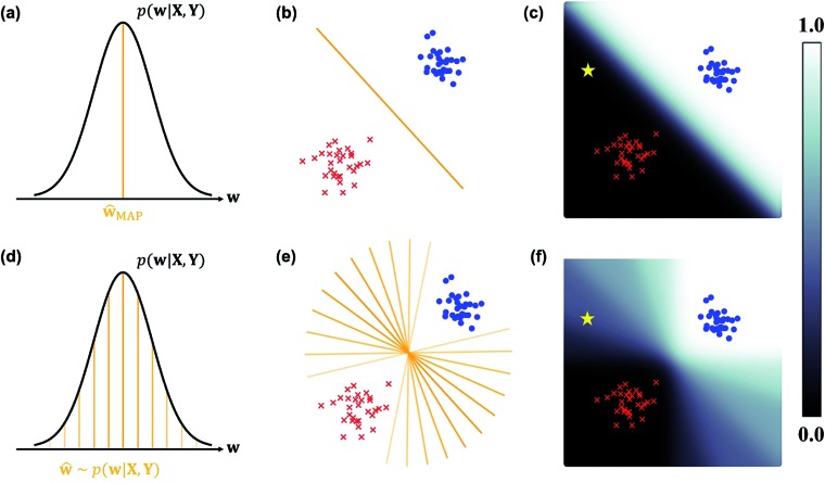
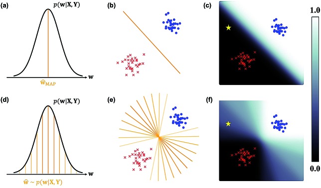
In the nature of a data-driven approach, a lack of qualified data can cause severe damage to the reliability of the prediction results of DNNs. This reliability issue should be taken more seriously when models are obtained by point estimation-based methods such as maximum-a-posteriori (MAP) or maximum likelihood (ML) estimation. It is because both estimation methods result in a single deterministic model which can produce unreliable outcomes for new data. In Fig. 1, we exemplify a drawback of using deterministic models for a classification problem with a small dataset. A small amount of data inevitably leads to a number of decision boundaries, which corresponds to a distribution of models, and the MAP (or ML) estimation selects only one from the distribution as shown in Fig. 1(a) and (b). In addition, the magnitude of output values is often erroneously interpreted as the confidence of prediction, and thus higher values are usually believed to be closer to the true value. That being said, relying on predicted outputs to make decisions can produce unreliable results for a new sample located far away from the distribution of training data. We illustrate an example of vulnerable decision making in Fig. 1(c). On one hand, the sample denoted by the yellow star will be predicted to belong to the red sample with nearly zero output probability according to the decision boundary estimated by the MAP. On the other hand, such a decision can be reversed by another possible decision boundary with the same accuracy for the given training data. As such, deterministic models can lead to catastrophic decisions in real-life applications, such as autonomous vehicle and medical fields, that put emphasis on so-called AI-safety problems.25–27
Fig. 1. A simple linearly separable binary classification problem. Positive and negative training data samples are denoted with blue and red markers, respectively. (a) A model estimated by MAP, ŵMAP, corresponds to the w value of the orange line, and (b) the decision boundary in the two-dimensional space is denoted by the orange line. (c) Output probability values (eqn (3)) are colored in the background. The orange lines with different transparency in (d) are models drawn from the posterior p(w|X, Y), and the lines in (e) are the corresponding decision boundaries. (f) Predictive probabilities obtained with Bayesian inference (eqn (4)) are colored in the background. The yellow star in (c) and (f) is a new unlabeled sample.
Collecting large amounts of data is one definite way to overcome the aforementioned problem but is usually expensive, time-consuming and laborious. Instead, Bayesian inference of model parameters and outputs enables more informative decision making by considering all possible outcomes predicted from the distribution of decision boundaries. In Fig. 1(d)–(f), we describe how to classify the yellow star according to Bayesian inference. Since various model parameters sampled from the posterior distribution will give different answers, the final outcome is obtained by averaging those answers. In addition, uncertainty quantification of prediction results is feasible thanks to the probabilistic nature of Bayesian inference. Kendall and Gal performed quantitative uncertainty analysis on computer vision problems by using DNNs grounded on a Bayesian framework.28 In particular, they have shown that the uncertainty of predictions can be decomposed into model- and data-driven uncertainties, which helps to identify the sources of prediction errors and further to improve both data and models.29 It has been known that results from Bayesian inference become identical to those of MAP estimation in the presence of a sufficiently large amount of data.30 However, as long as the amount of data is not enough like in most real-life applications, Bayesian inference would be more relevant.
In this work, we show that Bayesian inference is more informative in making reliable predictions than the standard ML estimation method. As a practical approach to obtain a distribution of model parameters and the corresponding outputs, we propose to exploit Bayesian neural networks. Since graph representation of molecular structures has been widely used, we chose molecular graphs as inputs for our model and implemented a graph convolutional network (GCN)31–33 within the Bayesian framework28,34 for the end-to-end learning of representations and predicting molecular properties.
The resulting Bayesian GCN is applied to the following four examples. In binary classification of bio-activity and toxicity, we show that prediction with a lower uncertainty turned out to be more accurate, which indicates that predictive uncertainty can be regarded as the confidence of prediction. Based on this finding, we carried out a virtual screening of drug candidates and found more known active molecules when using the Bayesian GCN than when using the same GCN model but estimating by the ML. The third example demonstrates that the uncertainty quantification enables us to separately analyze data-driven and model-driven uncertainties. Finally, we could identify artefacts in the synthetic power conversion efficiency values of molecules in the Harvard Clean Energy Project dataset.23 We verified that molecules with conspicuously large data-driven uncertainties were incorrectly annotated because of inaccurate approximations. Our results show that more reliable predictions can be achieved using Bayesian neural networks followed by uncertainty analysis.
2. Theoretical background
This section aims to explain the theoretical background of Bayesian neural networks. We first brief about Bayesian inference of model parameters and output to elaborate on our motivation of this research. Then, we briefly discuss variational inference as a practical approximation for implementation of Bayesian neural networks. Lastly, we explain a uncertainty quantification method based on Bayesian inference.
2.1. Bayesian inference of model parameters and output
Training a DNN is a procedure to obtain model parameters that best explain a given dataset. The Bayesian framework underlines that it is impossible to estimate a single deterministic model parameter, and hence one needs to infer the distribution of model parameters. For a given training set {X, Y}, let p(Y|X, w) and p(w) be a model likelihood and a prior distribution for a parameter w ∈ Ω, respectively. Following Bayes' theorem, a posterior distribution, which corresponds to the conditional distribution of model parameters given the training dataset, is defined as
 |
1 |
By using eqn (1), two different approaches have been derived: (i) MAP-estimation‡ finds the mode of the posterior and (ii) Bayesian inference computes the posterior distribution itself. The MAP estimated model ŵMAP is given by
 |
2 |
which is illustrated by the orange line in Fig. 1(a). Then, the expectation of output y* for a new input x* is given by
 |
3 |
where is fŵMAP(·) a function parameterized with ŵMAP. For instance, the orange line in Fig. 1(b) denotes the decision boundary, fŵMAP(·) = 0.5, in a simple linearly separable binary classification problem. The background color in Fig. 1(c) represents the output probability that a queried sample has a positive label (blue circle). Note that the right-hand-side term in eqn (3) does not have any conditional dependence on the training set {X, Y}.
In contrast to the MAP estimation, the Bayesian inference of outputs is given by the predictive distribution as follows:
 |
4 |
This formula allows more reliable predictions by the following two factors. First, the final outcome is inferred by integrating all possible models and their outputs. Second, it is possible to quantify the uncertainty of the predicted results. Fig. 1(d)–(f) illustrate the posterior distribution, sampled decision boundaries, and the resultant output probabilities, respectively. The new input denoted by the yellow star in Fig. 1(f) can be labeled differently according to the sampled model. Since the input is far away from the given training set, it is inherently difficult to assign a correct label without further information. As a result, the output probability is substantially low, and a large uncertainty of the prediction arises, as indicated by the gray color which is in contrast to the dark black color in Fig. 1(c). This conceptual example demonstrates the importance of the Bayesian framework especially in a limited data environment.
2.2. Variational inference in Bayesian neural networks
Direct incorporation of eqn (4) is intractable for DNN models because of heavy computational costs in the integration over the whole parameter space Ω. Diverse approximation methods have been proposed to mitigate this problem.35 We adopted a variational inference method which approximates the posterior distribution with a tractable distribution qθ(w) parameterized by a variational parameter θ.36,37 Minimizing the Kullback–Leibler divergence,
 |
5 |
makes the two distributions similar to one another in principle. We can replace the intractable posterior distribution in eqn (5) with p(Y∣X, w)p(w) by following Bayes' theorem in eqn (1). Then, our minimization objective, namely the negative evidence lower-bound, becomes
 |
6 |
For implementation, the variational distribution qθ(w) should be chosen carefully. Blundell et al. proposed to use a product of Gaussian distributions for the variational distribution qθ(w). In addition, a multiplicative normalizing flow38 can be applied to increase the expressive power of variational distribution. However, these two approaches require a large number of weight parameters. The Monte-Carlo dropout (MC-dropout) approximates the posterior distribution by a product of the Bernoulli distribution,39 the so-called dropout40 variational distribution. The MC-dropout is practical in that it does not need extra learnable parameters to model the variational posterior distribution, and the integration over the whole parameter space can be easily approximated with the summation of models sampled using a Monte-Carlo estimator.25,39
In practice, optimizing Bayesian neural networks with the MC-dropout, the so-called MC-dropout networks, is technically equivalent to that of standard neural networks with dropout as regularization. Hence, the training time for the MC-dropout networks is comparable to that for standard neural networks, which enables us to develop Bayesian neural networks with high scalability. In contrast to standard neural networks that predict outputs by turning-off the dropout at the inference phase, the MC-dropout networks keep turning on the dropout and predict outputs by sampling and averaging them, which theoretically corresponds to integrating the posterior distribution and likelihood.25 This technical simplicity provides an efficient way of Bayesian inference with neural networks. On the other hand, approximated posteriors implemented by the dropout variational inference often show inaccurate results, and several studies have reported the drawbacks of the MC-dropout networks.38,41,42 In this work, we focus on the practical advantages of the MC-dropout networks and introduce the Bayesian inference of molecular properties with graph convolutional networks.
2.3. Uncertainty quantification with a Bayesian neural network
A variational inference with an approximated variational distribution qθ(w) provides the (variational) predictive distribution of a new output y* given a new input x* as
 |
7 |
where fw(x*) is a model output with a given w. For regression tasks, a predictive mean of this distribution with T times MC sampling is estimated as
 |
8 |
and a predictive variance is estimated as
 |
9 |
with ŵt drawn from qθ(w) at the sampling step t and an assumption p(y*∣fw(x*)) = N(y*; fw(x*), σ2I). Here, the model assumes homoscedasticity with a known quantity, meaning that every data point gives a distribution with the same variance σ2. Further, obtaining the distributions with different variances allows deduction of a heteroscedastic uncertainty. Assuming the heteroscedasticity, the output given the t-th sample ŵt is
 |
10 |
Then, the heteroscedastic predictive uncertainty is given by eqn (11), which can be partitioned into two different uncertainties: aleatoric and epistemic uncertainties.
 |
11 |
The aleatoric uncertainty arises from data inherent noise, while the epistemic uncertainty is related to the model incompleteness.43 Note that the latter can be reduced by increasing the amount of training data, because it comes from an insufficient amount of data as well as the use of an inappropriate model.
In classification problems, Kwon et al. proposed a natural way to quantify the aleatoric and epistemic uncertainties as follows.
 |
12 |
where 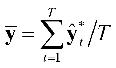 and
and  . While Kendall and Gal's method requires extra parameters σ̂t at the last hidden layer and often causes unstable parameter updates in a training phase,28 the method proposed by Kwon et al. has advantages in that models do not need the extra parameters.34Eqn (12) also utilizes a functional relationship between the mean and variance of multinomial random variables.
3. Methods
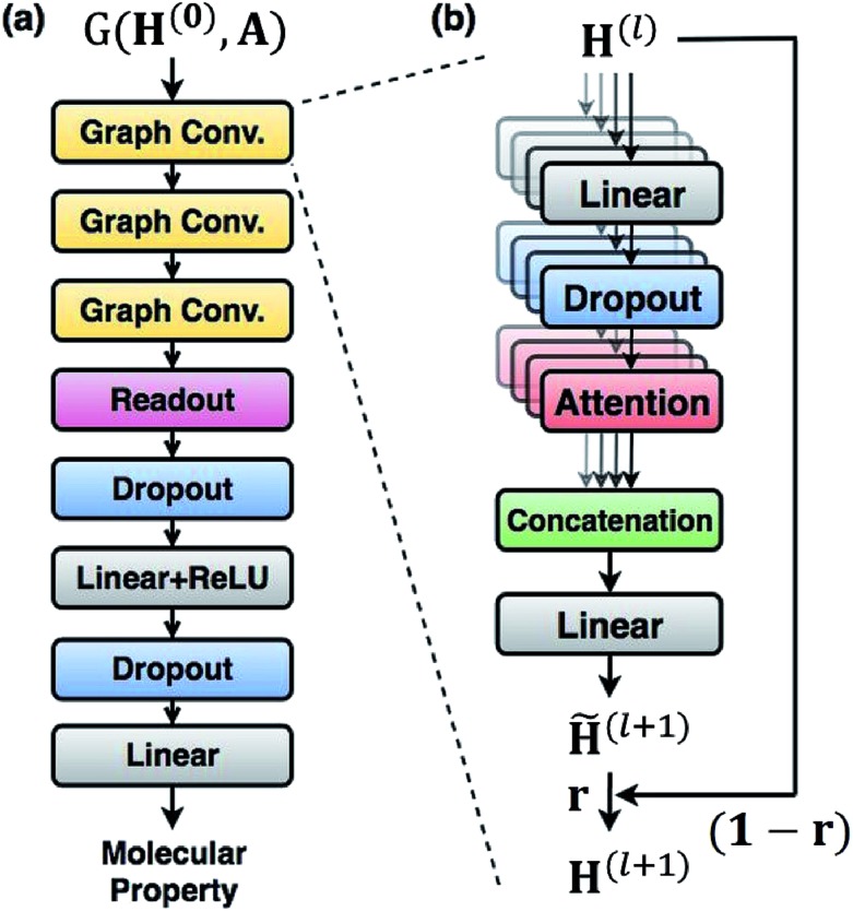
For predicting molecular properties, we adopt molecular graphs as input and the GCN augmented with attention and the gated mechanism suggested by Ryu et al.33 As illustrated in Fig. 2, the Bayesian GCN used in this work consists of the following three parts:
Fig. 2. The architecture of the Bayesian GCN used in this work. (a) The entire model is composed of three augmented graph convolutional layers, readout layers and two linear layers and takes inputs as a molecular graph G(H(0), A), where H0 is a node feature and A is an adjacency matrix. (b) Details of each graph convolution layer augmented with attention and gate mechanisms. The l-th graph convolutional layer updates node features and produces H(l+1).
• Three augmented graph convolution layers update node features. The number of self-attention heads is four. The dimension of output from each layer is (75 × 32).
• A readout function produces a graph feature whose dimension is 256.
• A feed-forward MLP, which is composed of two fully connected layers, outputs a molecular property. The hidden dimension of each fully connected layer is 256.
In order to approximate the posterior distribution with a dropout variational distribution, we applied dropouts at every hidden layer. We did not use the standard dropout with a hand-tuned dropout rate but used Concrete dropout44 to develop as accurate Bayesian models as possible. By using the Concrete dropout, we can obtain the optimal dropout rate for individual hidden layers by gradient descent optimization. We used Gaussian priors 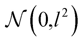 with a length scale of l = 10–4 for all model parameters. In the training phase, we used the Adam optimizer45 with an initial learning rate of 10–3, and the learning rate decayed by half every 10 epochs. The number of total training epochs is 100, and the batch size is 100. We randomly split each dataset in the ratio of 0.72 : 0.08 : 0.2 for training, validation and testing. For all experiments, we kept turning on the dropout at the inference phases and sampled outputs with T = 20 (in eqn (8), (9) and (12)) and averaged them in order to perform Bayesian inference. We used one GTX-1080 Ti processor for performing all experiments. We provide the number of samples used for training/validation/testing, training time, and accuracy curves for all experiments in the ESI.† The code used for the experiments is available at ; https://github.com/seongokryu/uq_molecule.
4. Results and discussion
4.1. Relationship between the uncertainty and output probability: bio-activity and toxicity classification
In classification problems, the output probability itself tends to be regarded as the confidence of prediction. For example, in a virtual screening of drug candidates, molecules predicted to be active with high output probability are preferred. However, as Gal and Ghahramani pointed out, such interpretation is erroneous for deterministic models.39Fig. 1(c) shows such an example. Indeed, though the MAP-estimated model can give a high output probability to a sample located far away from the distribution of training data, it is difficult to determine its correct label due to lack of information. In contrast, Bayesian inference allows us to obtain predictive uncertainty as well as output probabilities. In the case of the yellow star, the Bayesian inference gives a low output probability with high predictive uncertainty as expected. With two biological classification problems having a limited amount of data, we here show that the higher the output probability of the Bayesian GCN is, the lower the predictive uncertainty and hence predictive uncertainty can be regarded as the confidence of prediction.
We trained the Bayesian GCN with 25 627 molecules which are annotated with EGFR inhibitory activity in the DUD-E dataset. Fig. 3 shows the relationship between predictive uncertainty and output probability for 7118 molecules in the test set. The total uncertainty as well as the aleatoric and epistemic uncertainties are minimum at both highest and lowest output probabilities, while they are maximum at the center. Therefore, one can make a confident decision by taking the highest or lowest output probabilities; however it should be emphasized again that this is not the case for the MAP- or ML-estimated models.
Fig. 3. (a) Aleatoric, (b) epistemic and (c) total uncertainty with respect to the output probability in the classification of EGFR inhibitory activity.
Based on this finding, uncertainty calibrated decision making can lead to high accuracy in classification problems. To verify this, we trained the Bayesian GCNs with bio-activity labels for various target proteins in the DUD-E dataset and toxicity labels in the Tox21 dataset. Then, we sorted the molecules in increasing order of uncertainty and divided them into five groups as follows: molecules in the i-th group have total uncertainties in the range of [(i – 1) × 0.1, i × 0.1]. Fig. 4(a) and (b) show the accuracy of each group for five different bio-activities in the DUD-E dataset and five different toxicities in the Tox21 dataset, respectively. For all cases, the first group having the lowest uncertainty showed the highest accuracy. This result manifests that the uncertainty values can be used as a confidence indicator.
Fig. 4. Test accuracy for the classifications of (a) bio-activities against the five target proteins in the DUD-E dataset and (b) the five toxic effects in the Tox21 dataset.
4.2. Virtual screening of EGFR inhibitors in the ChEMBL dataset
We have shown that confident predictions of molecular properties have become feasible thanks to the relationship between the output probability and predictive uncertainty within the Bayesian framework. Here, we examine whether such an uncertainty-calibrated prediction can lead to higher accuracy in real-life applications than a maximum likelihood (ML) and a maximum-a-posteriori (MAP) estimation approach. To this end, we applied the previous Bayesian GCN trained with the DUD-E dataset to the virtual screening of EGFR inhibitors in the ChEMBL dataset.46 We deliberately used two completely different datasets for training and testing so as to evaluate the generalization ability of the model.
Molecules in the ChEMBL dataset were annotated with an experimental half maximal inhibitory concentration (IC50) value. To utilize this dataset for a classification problem, we assigned molecules with IC50 values above 6.0 as ground truth active, while the others were assigned as ground truth inactive. We compare three GCN models obtained by three different estimation methods: (i) ML, (ii) MAP, and (iii) Bayesian. We turned off the dropout masks and did not use MC-sampling at the inference phase to obtain the MAP-estimated GCN. Also, we obtained the ML-estimated GCN with the same training configurations except the dropout and L2-regularization. Then, we applied the three models to the virtual screening of the ChEMBL dataset.
Table 1 summarizes the screening results of the three models in terms of accuracy, area under receiver operating curve (AUROC), precision, recall and F1-score. The Bayesian GCN outperformed the point-estimated GCNs for all evaluation metrics except the recall. Since Bayesian inference assumes a model prior which corresponds to the regularization term in the training procedure, the Bayesian GCN showed better generalization ability and performance than the ML-estimated GCN as it was applied to the unseen dataset.36 In contrast to the MAP-estimated GCN, whose model parameter (or decision boundary) is point-estimated, the Bayesian GCN infers predictive probability by MC-sampling of outputs with different dropout masks. This inference procedure allows the model to predict outputs by considering a multiple number of decision boundaries and shows better performance in the virtual screening experiment.
Table 1. Performance of the GCN models obtained by different estimation methods in predicting the EGFR-inhibitory activity of molecules in the ChEMBL dataset.
| ML | MAP | Bayesian | |
| Accuracy | 0.728 | 0.739 | 0.752 |
| AUROC | 0.756 | 0.781 | 0.785 |
| Precision | 0.714 | 0.68 | 0.746 |
| Recall | 0.886 | 0.939 | 0.868 |
| F1-score | 0.791 | 0.789 | 0.803 |
In Fig. 5, we visualize the distribution of output probability by dividing it into true positive, false positive, true negative and false negative groups. The output probability values of the ML-estimated GCN is close to 0.0 or 1.0 for most molecules, which is commonly referred to as over-confident prediction. Because of the regularization effect, the MAP-estimated GCN shows less over-confident results than the ML-estimated GCN. On the other hand, the outputs of the Bayesian GCN are distributed continuously from 0.0 to 1.0. This result is consistent with the previous conclusion that the Bayesian GCN predicts a value between 0.0 and 1.0 according to the extent of the predictive uncertainty for a given sample.
Fig. 5. Distributions of output probability obtained by (a) the ML, (b) the MAP and (c) the Bayesian GCNs. The total distribution is divided into true positive (blue), false positive (orange), true negative (green) and false negative (red) groups. Note that the y-axis is represented with a log scale.
As demonstrated in the previous section, with Bayesian inference, an output probability value closer to one is expected more likely to be a true active label. This allows output probability to be used as a criterion for screening of desirable molecules. Table 2 shows the number of actives existing in each list of the top 100, 200, 300 and 500 molecules in terms of output probability. The Bayesian GCN mined remarkably more active molecules than the ML-estimated GCN did. In particular, it performed better in the top 100 and 200, which is critical for efficient virtual screening purposes with a small amount of qualified data. Also, it performed slightly better than the MAP-estimated GCN for all trials.
Table 2. The number of actives existing in the top N molecules that are sorted in increasing order of output probability.
| Top N | ML | MAP | Bayesian |
| 100 | 29 | 57 | 69 |
| 200 | 67 | 130 | 140 |
| 300 | 139 | 202 | 214 |
| 500 | 277 | 346 | 368 |
4.3. Implication of data quality on aleatoric and epistemic uncertainties
In this experiment, we investigated how data quality affects predictive uncertainty. In particular, we analyzed the aleatoric and epistemic uncertainties separately in molecular property predictions using the Bayesian GCN. We chose log P prediction as an example because we can obtain a sufficient amount of logP values by using a deterministic formulation in the RDKit.47 We assumed that these log P values do not include noise (stochasticity) and let them be ground truth labels. In order to control the data quality, we adjusted the extent of noise by adding a random Gaussian noise 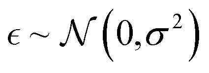 . Then, we trained the model with 97 287 samples and analyzed uncertainties of each predicted log P for 27 023 samples.
Fig. 6 shows the distribution of the three uncertainties with respect to the amount of additive noise σ2. As the noise level increases, the aleatoric and total uncertainties increase, but the epistemic uncertainty is slightly changed. This result verifies that the aleatoric uncertainty arises from data inherent noises, while the epistemic uncertainty does not depend on data quality. Theoretically, the epistemic uncertainty should not be increased by the changes in the amount of data noise. Presumably, stochasticity in the numerical optimization of model parameters induced the slight change of the epistemic uncertainty.
Fig. 6. Histograms of (a) aleatoric, (b) epistemic and (c) total uncertainties as the amount of additive noise σ2 increases.
4.4. Evaluating the quality of synthetic data based on uncertainty analysis
Based on the analysis of the previous experiment, we attempted to see whether uncertainty quantification can be used to evaluate the quality of existing chemical data.
Synthetic PCE values in the CEP dataset23 were obtained from the Scharber model with statistical approximations.48 In this procedure, unintentional errors can be included in the resulting synthetic data. Therefore, this example would be a good exercise problem to evaluate the quality of data through the analysis of aleatoric uncertainty. We used the same dataset of Duvenaud et al.§ for training and testing.
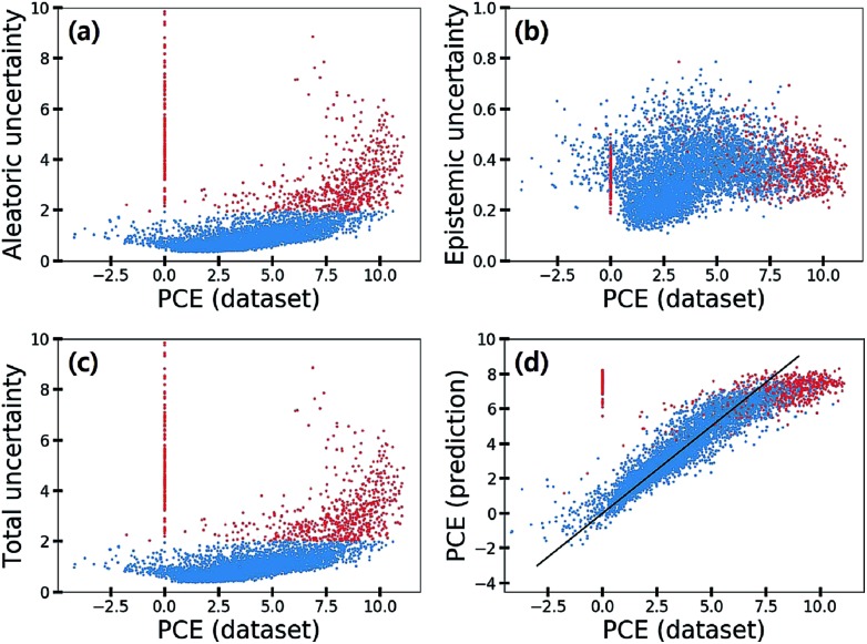
Fig. 7 shows the scatter plot of three uncertainties in the CEP predictions for 5995 molecules in the test set. Samples with a total uncertainty greater than two are highlighted with red color. Some samples with large PCE values above eight had relatively large total uncertainties. Their PCE values deviated considerably from the black line in Fig. 7(d). Notably most molecules with a zero PCE value had large total uncertainties as well. These large uncertainties came from the aleatoric uncertainty as depicted in Fig. 7(a), indicating that the data quality of these particular samples is relatively poor. Hence, we speculated that data inherent noises might cause large prediction errors.
Fig. 7. (a) Aleatoric, (b) epistemic, and (c) total uncertainties and (d) predicted PCE value against the PCE value in the dataset. The samples colored in red show a total uncertainty greater than two.
To elaborate the origin of such errors, we investigated the procedure of obtaining the PCE values. The Harvard Organic Photovoltaic Dataset49 contains both experimental and synthetic PCE values of 350 organic photovoltaic materials. The synthetic PCE values were computed according to eqn (13), which is the result of the Scharber model.48
| PCE ∝ VOC × FF × JSC, | 13 |
where VOC is the open circuit potential, FF is the fill factor, and JSC is the short circuit current density. FF was set to 65%. VOC and JSC were obtained from electronic structure calculations of molecules.23 We found that the JSC of some molecules were zero or nearly zero, which might be from the artefact of quantum mechanical calculations. In particular, in contrast to their non-zero experimental PCE values, JSC and PCE values computed by using the M06-2X functional50 were almost zero consistently. Pyzer-Knapp et al. pointed out this problem and proposed a statistical calibration method that can successfully correct the biased results.51
To summarize, we suspect that quantum mechanical artefacts caused a significant drop of data quality, resulting in the large aleatoric uncertainties as highlighted in Fig. 7. Consequently, we can identify data inherent noise by analyzing aleatoric uncertainty.
5. Conclusion
Deep neural networks (DNNs) have shown promising success in the prediction of molecular properties as long as a large amount of data is available. However, a lack of qualified data in many chemical problems discourages employing them directly due to the nature of a data-driven approach. In particular, deterministic models, which can be derived from maximum likelihood (ML) or maximum-a-posteriori (MAP) estimation methods, may cause vulnerable decision making in real-life applications where reliable predictions are very important.
Here, we have studied the possibility of reliable predictions and decision making in such cases with the Bayesian GCN. Our results show that output probability from the Bayesian GCN can be regarded as the confidence of prediction in classification problems, which is not the case for the ML- or MAP-estimated models. Moreover, we demonstrated that such a confident prediction can lead to notably higher accuracy for a virtual screening of drug candidates than a standard approach based on the ML-estimation. In addition, we showed that uncertainty analysis enabled by Bayesian inference can be used to evaluate data quality in a quantitative manner and thus helps to find possible sources of errors. As an example, we could identify unexpected errors included in the Harvard Clean Energy Project dataset and their possible origin using the uncertainty analysis. Most chemical applications of deep learning have adopted DNN models estimated by either MAP or ML. Our study clearly shows that Bayesian inference is essential in limited data environments where AI-safety problems are critical.
Beyond reliable prediction of molecular properties along with uncertainty quantification, we expect that DNNs with the Bayesian perspective may be extended to data-efficient algorithms for molecular applications. One of the possible interesting future applications is to use Bayesian GCNs for high-throughput screening of chemical space with Bayesian optimization.52 For this purpose, Bayesian optimization has been utilized as a promising tool to search for the most desirable candidates based on predictive uncertainty.6,53–55 In chemistry, Hernández-Lobato et al. proposed a computationally efficient Bayesian optimization framework that was built on a Gaussian process with Morgan fingerprints as inputs for the estimation of predictive uncertainty.55 Thus, we believe that our proposed method has potential for designing efficient high-throughput screening tools for drug or materials discovery.
Another important possible application of Bayesian GCNs is extension for active learning. Since acquiring big data from experiments is expensive and laborious, data-efficient learning algorithms are attracting attention as a viable solution in various real-life applications by enabling neural networks to be trained with a small amount of data.56 Active learning, is one of such algorithms, employs an acquisition function suggesting new data points that should be added for further improvement of model accuracy. Incorporation of the Bayesian framework in the active learning helps to select new data points by providing fruitful information with predictive uncertainty.29 In this regard, we believe that the present work offers insights into the development of a deep learning approach in a data-efficient way for various chemical problems, which hopefully promotes synergistic cooperation of deep learning with experiments.
Author contributions
S. R. and Y. K. conceived the idea. S. R. did the implementation and ran the simulation. All the authors analyzed the results and wrote the manuscript together.
Conflicts of interest
The authors declare no competing financial interests.
Supplementary Material
Acknowledgments
We would like to appreciate the anonymous reviewers for their constructive comments. This work was supported by the Basic Science Research Program through the National Research Foundation of Korea (NRF) funded by the Ministry of Science, ICT and Future Planning (NRF-2017R1E1A1A01078109).
Footnotes
†Electronic supplementary information (ESI) available. See DOI: 10.1039/c9sc01992h
‡We would like to note two things in the MAP estimation. First, eqn (2) can be computed by gradient descent optimization, which corresponds to the common training procedure of machine learning systems, minimizing a negative-log-likelihood term (a loss function) and a regularization term. Second, the MAP estimation becomes equivalent to the maximum likelihood estimation which maximizes the likelihood term only when we assume a uniform prior distribution.
References
- Gomes J., Ramsundar B., Feinberg E. N. and Pande V. S., 2017, arXiv preprint arXiv:1703.10603.
- Jiménez J., Skalic M., Martínez-Rosell G., De Fabritiis G. J. Chem. Inf. Model. 2018;58:287–296. doi: 10.1021/acs.jcim.7b00650. [DOI] [PubMed] [Google Scholar]
- Mayr A., Klambauer G., Unterthiner T., Hochreiter S. Front. environ. sci. 2016;3:80. [Google Scholar]
- Öztürk H., Özgür A., Ozkirimli E. Bioinformatics. 2018;34:i821–i829. doi: 10.1093/bioinformatics/bty593. [DOI] [PMC free article] [PubMed] [Google Scholar]
- De Cao N. and Kipf T., 2018, arXiv preprint arXiv:1805.11973.
- Gómez-Bombarelli R., Wei J. N., Duvenaud D., Hernández-Lobato J. M., Sánchez-Lengeling B., Sheberla D., Aguilera-Iparraguirre J., Hirzel T. D., Adams R. P., Aspuru-Guzik A. ACS Cent. Sci. . 2018;4:268–276. doi: 10.1021/acscentsci.7b00572. [DOI] [PMC free article] [PubMed] [Google Scholar]
- Guimaraes G. L., Sanchez-Lengeling B., Outeiral C., Farias P. L. C. and Aspuru-Guzik A., 2017, arXiv preprint arXiv:1705.10843.
- Jin W., Barzilay R. and Jaakkola T., 2018, arXiv preprint arXiv:1802.04364.
- Kusner M. J., Paige B. and Hernández-Lobato J. M., 2017, arXiv preprint arXiv:1703.01925.
- Li Y., Vinyals O., Dyer C., Pascanu R. and Battaglia P., 2018, arXiv preprint arXiv:1803.03324.
- Segler M. H., Kogej T., Tyrchan C., Waller M. P. ACS Cent. Sci. . 2017;4:120–131. doi: 10.1021/acscentsci.7b00512. [DOI] [PMC free article] [PubMed] [Google Scholar]
- You J., Liu B., Ying R., Pande V. and Leskovec J., 2018, arXiv preprint arXiv:1806.02473.
- Segler M. H., Preuss M., Waller M. P. Nature. 2018;555:604. doi: 10.1038/nature25978. [DOI] [PubMed] [Google Scholar]
- Wei J. N., Duvenaud D., Aspuru-Guzik A. ACS Cent. Sci. . 2016;2:725–732. doi: 10.1021/acscentsci.6b00219. [DOI] [PMC free article] [PubMed] [Google Scholar]
- Zhou Z., Li X., Zare R. N. ACS Cent. Sci. . 2017;3:1337–1344. doi: 10.1021/acscentsci.7b00492. [DOI] [PMC free article] [PubMed] [Google Scholar]
- Faber F. A., Hutchison L., Huang B., Gilmer J., Schoenholz S. S., Dahl G. E., Vinyals O., Kearnes S., Riley P. F., von Lilienfeld O. A. J. Chem. Theory Comput. 2017;13:5255–5264. doi: 10.1021/acs.jctc.7b00577. [DOI] [PubMed] [Google Scholar]
- Gilmer J., Schoenholz S. S., Riley P. F., Vinyals O. and Dahl G. E., 2017, arXiv preprint arXiv:1704.01212.
- Schütt K., Kindermans P.-J., Felix H. E. S., Chmiela S., Tkatchenko A. and Müller K.-R., Advances in Neural Information Processing Systems, 2017, pp. 991–1001. [Google Scholar]
- Schütt K. T., Arbabzadah F., Chmiela S., Müller K. R., Tkatchenko A. Nat. Commun. 2017;8:13890. doi: 10.1038/ncomms13890. [DOI] [PMC free article] [PubMed] [Google Scholar]
- Smith J. S., Isayev O., Roitberg A. E. Chem. Sci. 2017;8:3192–3203. doi: 10.1039/c6sc05720a. [DOI] [PMC free article] [PubMed] [Google Scholar]
- Feinberg E. N., Sur D., Husic B. E., Mai D., Li Y., Yang J., Ramsundar B. and Pande V. S., 2018, arXiv preprint arXiv:1803.04465.
- Liu Z., Su M., Han L., Liu J., Yang Q., Li Y., Wang R. Acc. Chem. Res. 2017;50:302–309. doi: 10.1021/acs.accounts.6b00491. [DOI] [PubMed] [Google Scholar]
- Hachmann J., Olivares-Amaya R., Atahan-Evrenk S., Amador-Bedolla C., Sánchez-Carrera R. S., Gold-Parker A., Vogt L., Brockway A. M., Aspuru-Guzik A. J. Phys. Chem. Lett. 2011;2:2241–2251. [Google Scholar]
- Mysinger M. M., Carchia M., Irwin J. J., Shoichet B. K. J. Med. Chem. 2012;55:6582–6594. doi: 10.1021/jm300687e. [DOI] [PMC free article] [PubMed] [Google Scholar]
- Gal Y., Uncertainty in Deep Learning, PhD thesis, University of Cambridge, 2016.
- McAllister R., Gal Y., Kendall A., van der Wilk M., Shah A., Cipolla R. and Weller A. V., Concrete Problems for Autonomous Vehicle Safety, Advantages of Bayesian Deep Learning, Proceedings of the Twenty-Sixth International Joint Conference on Artificial Intelligence AI and autonomy track, 2017, pp. 4745–4753. [Google Scholar]
- Begoli E., Bhattacharya T., Kusnezov D. Nat. Mach. Intell. 2019;1:20. [Google Scholar]
- Kendall A. and Gal Y., Advances in neural information processing systems, 2017, pp. 5574–5584. [Google Scholar]
- Gal Y., Islam R. and Ghahramani Z., Proceedings of the 34th International Conference on Machine Learning, 2017, vol. 70, pp. 1183–1192. [Google Scholar]
- Murphy K. P., Machine Learning: A Probabilistic Perspective, Adaptive Computation and Machine Learning series, 2018. [Google Scholar]
- Duvenaud D. K., Maclaurin D., Iparraguirre J., Bombarell R., Hirzel T., Aspuru-Guzik A. and Adams R. P., Advances in neural information processing systems, 2015, pp. 2224–2232. [Google Scholar]
- Kipf T. N. and Welling M., 2016, arXiv preprint arXiv:1609.02907.
- Ryu S., Lim J. and Kim W. Y., 2018, arXiv preprint arXiv:1805.10988.
- Kwon Y., Won J.-H., Kim B. J. and Paik M. C., international conference on medical imaging with deep learning, 2018. [Google Scholar]
- Gelman A., Stern H. S., Carlin J. B., Dunson D. B., Vehtari A. and Rubin D. B., Bayesian data analysis, Chapman and Hall/CRC, 2013. [Google Scholar]
- Blundell C., Cornebise J., Kavukcuoglu K. and Wierstra D., 2015, arXiv preprint arXiv:1505.05424.
- Graves A., Advances in neural information processing systems, 2011, pp. 2348–2356. [Google Scholar]
- Louizos C. and Welling M., 2017, arXiv preprint arXiv:1703.01961.
- Gal Y. and Ghahramani Z., international conference on machine learning, 2016, pp. 1050–1059. [Google Scholar]
- Srivastava N., Hinton G., Krizhevsky A., Sutskever I., Salakhutdinov R. J. mach. learn. res. 2014;15:1929–1958. [Google Scholar]
- Kuleshov V., Fenner N. and Ermon S., 2018, arXiv preprint arXiv:1807.00263.
- Gal Y. and Smith L., 2018, arXiv preprint arXiv:1806.00667.
- Der Kiureghian A., Ditlevsen O. Struct. Saf. 2009;31:105–112. [Google Scholar]
- Gal Y., Hron J. and Kendall A., Advances in Neural Information Processing Systems, 2017, pp. 3581–3590. [Google Scholar]
- Kingma D. P. and Ba J., 2014, arXiv preprint arXiv:1412.6980.
- Gaulton A., Hersey A., Nowotka M., Bento A. P., Chambers J., Mendez D., Mutowo P., Atkinson F., Bellis L. J., Cibrián-Uhalte E. Nucleic Acids Res. 2016;45:D945–D954. doi: 10.1093/nar/gkw1074. [DOI] [PMC free article] [PubMed] [Google Scholar]
- Landrum G., RDKit: Open-source cheminformatics, 2006. [Google Scholar]
- Scharber M. C., Mühlbacher D., Koppe M., Denk P., Waldauf C., Heeger A. J., Brabec C. J. Adv. Mater. 2006;18:789–794. [Google Scholar]
- Lopez S. A., Pyzer-Knapp E. O., Simm G. N., Lutzow T., Li K., Seress L. R., Hachmann J., Aspuru-Guzik A. Sci. Data. 2016;3:160086. doi: 10.1038/sdata.2016.86. [DOI] [PMC free article] [PubMed] [Google Scholar]
- Zhao Y., Truhlar D. G. Theor. Chem. Acc. 2008;120:215–241. [Google Scholar]
- Pyzer-Knapp E. O., Simm G. N., Guzik A. A. Mater. Horiz. 2016;3:226–233. [Google Scholar]
- Jones D. R., Schonlau M., Welch W. J. J. Glob. Optim. 1998;13:455–492. [Google Scholar]
- Griffiths R.-R. and Hernández-Lobato J. M., 2017, arXiv preprint arXiv:1709.05501.
- HaÌĹse F., Roch L. M., Kreisbeck C., Aspuru-Guzik A. ACS Cent. Sci. . 2018;4:1134–1145. doi: 10.1021/acscentsci.8b00307. [DOI] [PMC free article] [PubMed] [Google Scholar]
- Hernández-Lobato J. M., Requeima J., Pyzer-Knapp E. O. and Aspuru-Guzik A., Proceedings of the 34th International Conference on Machine Learning, 2017, vol. 70, pp. 1470–1479. [Google Scholar]
- Cohn D. A., Ghahramani Z., Jordan M. I. J. Artif. Intell. Res. 1996;4:129–145. [Google Scholar]
Associated Data
This section collects any data citations, data availability statements, or supplementary materials included in this article.


