Regionally strong feedbacks between the atmosphere and terrestrial biosphere

Abstract

The terrestrial biosphere and atmosphere interact through a series of feedback loops. Variability in terrestrial vegetation growth and phenology can modulate fluxes of water and energy to the atmosphere, and thus affect the climatic conditions that in turn regulate vegetation dynamics. Here we analyze satellite observations of solar-induced fluorescence, precipitation, and radiation using a multivariate statistical technique. We find that biosphere-atmosphere feedbacks are globally widespread and regionally strong: they explain up to 30% of precipitation and surface radiation variance. Substantial biosphere-precipitation feedbacks are often found in regions that are transitional between energy and water limitation, such as semi-arid or monsoonal regions. Substantial biosphere-radiation feedbacks are often present in several moderately wet regions and in the Mediterranean, where precipitation and radiation increase vegetation growth. Enhancement of latent and sensible heat transfer from vegetation accompanies this growth, which increases boundary layer height and convection, affecting cloudiness, and consequently incident surface radiation. Enhanced evapotranspiration can increase moist convection, leading to increased precipitation. Earth system models underestimate these precipitation and radiation feedbacks mainly because they underestimate the biosphere response to radiation and water availability. We conclude that biosphere-atmosphere feedbacks cluster in specific climatic regions that help determine the net CO₂ balance of the biosphere.

By influencing the partitioning of turbulent fluxes at the surface¹, soil moisture and temperature can affect climatic variability². Biospheric variability, in terms of both phenology and stomatal regulation, also strongly modulates turbulent fluxes of both water and energy³. Since biospheric variability is regulated by vegetation phenology and root zone soil moisture, it exhibits longer (e.g. multi-month) memory compared to the more commonly studied surface soil moisture and temperature state. Therefore, an understanding of biosphere-atmosphere interactions has the potential to improve seasonal to interannual climatic predictions^4,5,6, and improve predictions of vegetation resilience to climate anomalies⁷. However, global variations in the strength of biosphere-atmosphere feedbacks remain unknown, in part because of the difficulty of observing biospheric fluxes⁸.

Recent advancements in space-borne observations of solar-induced fluorescence (SIF) have enabled for the first-time a global proxy for gross primary productivity (GPP) and vegetation phenology. SIF is a by-product of photosynthesis⁹ related to light-use efficiency (LUE) and to the fraction of absorbed photosynthetic active radiation (fAPAR)¹⁰. On a canopy or regional scale and at a monthly resolution it is nearly proportional to GPP across various ecosystems. This large-scale correspondence is strongly related to the changes in canopy structure and phenology on absorbed photosynthetic active radiation, in addition to the more subtle changes in LUE^11,12,13,14. SIF is also generally highly correlated with evapotranspiration (ET)¹⁵ (Supplementary Fig. 1) and correlates with vegetation-driven changes in surface albedo. Here, we use SIF as an integrated measure of vegetation variability, capturing both growth and changes in photosynthetic capacity (Methods).

Previous studies of land-atmosphere interactions have typically relied on correlations between land and atmospheric variables^16,17,18. However, these variables seasonally coevolve, and thus it is difficult to determine whether one variable is causally forcing the other, or if the two are both driven by separate factors^19,20. Here, these shortcomings are overcome by employing a Multivariate Conditional Granger causality (MVGC) statistical technique using vector autoregressive models (VARs)²¹. This method determines both the strength of the predictive mechanism between variables and the time scale over which these links occur (Methods).

MVGC observational data forcings

We apply the MVGC VAR statistical technique to eight years of monthly SIF measurements from the Global Ozone Monitoring Experiment 2 (GOME-2) sensor²². SIF-precipitation interactions are assessed using remote sensing-based estimates from the Global Precipitation Climatology Project (GPCP)²³ and SIF-radiation interactions are assessed using photosynthetic active radiation (PAR) from Clouds and the Earth’s Radiant Energy System (CERES)²⁴. We also use surface air temperature reanalysis data from ERA-Interim²⁵, as temperature can independently impact and interact with photosynthetic activity¹⁸. SIF data is relatively noisy, and thus spatial averaging is used to smooth it prior to analysis (Methods). It should be acknowledged that the smoothing could distort results in highly heterogeneous regions where signals from various biomes may be aggregated. Note that, although the linear scaling factor between monthly SIF and GPP varies between ecosystems and climates¹² the pixel-by-pixel data normalization used here removes the geographical variations of this factor (Methods). The analysis presented here is independent of the scaling factor.

To identify biosphere-atmosphere coupled feedbacks, we first examine their directional sub-components, i.e. the atmospheric forcing (atmosphere biosphere), as assessed by the response of SIF (GPP) to atmospheric drivers (the fraction of variance in SIF explained by precipitation and PAR), and the biospheric forcing (biosphere atmosphere), as assessed by precipitation and PAR response to SIF (the fraction of variance in precipitation and PAR explained by SIF) (Fig. 1). An F-test with a null-hypothesis of 0-Granger causality (G-causality) (p-value <0.1) is used. The total feedback strength is then defined as the product of these two directional components (Fig. 2). The sign of the feedback is defined as the sign of the first order coefficient of the VAR model from the G-causality analysis. To ensure the results presented here are robust and independent of the seasonal cycle (i.e. due to land-atmosphere interactions), a bootstrap test that conserves the seasonal cycle but breaks the causality by shuffling months from different years is used (Supplementary Fig. 2) and clearly destroys the feedback.

Figure 1. Atmospheric forcings and biospheric forcings.

X Y represents the fraction of variance of Y explained by X, for the atmospheric forcing (atmosphere biosphere) (a,c), and biospheric forcing (biosphere atmosphere) (b,d). The signs of the fractions in the top row show whether the atmospheric variable increases (positive) or decreases (negative) the biosphere flux, while in the bottom row they show whether the biosphere increases or decreases the atmospheric response. Oceans and regions where SIF partial correlations are less than 0.1 are shown in white. Pixels without significance are shown in gray (p-value<0.1).

Fig. 2. Hotspots of terrestrial biosphere-atmosphere feedbacks.

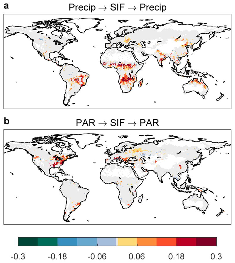
The fraction of biosphere-atmosphere coupling variance explained for the full feedback loop: precipitation SIF precipitation (a) and PAR SIF PAR (b). The sign of the fraction shows whether the feedback is positive or negative. Oceans and regions where SIF partial correlations are less than 0.1 are shown in white. Pixels without significance are shown in gray (p-value<0.1).

Globally, precipitation positively explains the highest fraction of biosphere (SIF) variability in regions that are transitional between wet and dry climates, e.g. semi-arid or monsoonal (Fig. 1a), consistent with previous studies^7,16. Many of these regions also have high fractions of C4 plants²⁶, which have higher water use efficiency than C3 species²⁷, and are therefore expected to be more sensitive to water limitations. The impact of the biosphere on precipitation (Fig. 1b), as assessed by the G-causality of SIF on precipitation, is seen in seasonally dry regions where increases in GPP, in response to increased soil moisture and vegetation growth, is linked with higher latent heat flux and reduced sensible heat flux (Supplementary Fig. 1). Although the impact of SIF on precipitation is less widespread than that of precipitation on SIF, it is significant in many of the same regions. The feedbacks are almost always positive because the monthly positive effect of evapotranspiration on moist convection dominates negative feedback pathways induced by mesoscale surface heterogeneity²⁸ and the effects of changing albedo. The time scales involved in the feedback mechanisms can vary between regions. The subseasonal signal may represent variability due to early greening induced by increased water supply or to browning induced by water stress, while seasonal and interannual signals may indicate changes in vegetation growth regulated by water availability during cell division. The strongest signals are detected subseasonally in monsoonal Australia, seasonally in Eastern Asia, and both seasonally and interannually in the Sahel and Southern African Monsoonal regions (Supplementary Fig. 3). The dominance of seasonal and interannual time scales in the Sahel, related to biomass variability, is consistent with previous understanding^6,29.

PAR has the greatest impact on biosphere fluxes (Fig. 1c) in regions where photosynthesis and vegetation growth is energy limited such as the high latitudes, humid regions of the Eastern US, parts of the Mediterranean, and tropical rainforest regions^30,31. This agrees with the findings of previous studies showing that net primary production (NPP) in these regions is driven by radiation¹⁸. The biosphere exerts control on PAR in the Eastern US, central Eurasia, African deciduous woodlands as well as in the European Mediterranean region (Fig. 1d). In these very dry or very wet regions, ecosystems rarely enter the transitional regime where stomatal closure depends on soil moisture, and increases in SIF are accompanied by increases in both sensible and latent heat (Supplementary Fig. 1)³². The increased sensible heat flux leads to a deeper boundary layer and reduced cloud cover (Supplementary Fig. 4), therefore increasing PAR (Fig. 1d). In the Eastern US, the increase in PAR is mostly attributed to a reduction of low- and mid-level (i.e. congestus) cumulus clouds, typical of summer conditions in this humid climate (Supplementary Fig. 4). By contrast, in the European Mediterranean, PAR is most sensitive to mid- and high-level clouds. In central Eurasia all cloud cover levels negatively impact surface PAR but high-level clouds are the primary reason for the PAR change. The strongest feedbacks between SIF and PAR tend to be on a seasonal scale indicating an increase in ecosystem-scale photosynthetic capacity due to vegetation growth, with exceptions in Madagascar, Australia and central Eurasia where subseasonal and interannual feedbacks dominate (Supplementary Fig. 3). In all PAR feedback regions, PAR is also negatively correlated with precipitation (Supplementary Fig. 4). We note that the European Mediterranean has been highlighted as a hotspot of land-atmosphere coupling in an earlier modeling study, emphasizing the strong coupling between surface turbulent fluxes and the boundary layer response in the region³³. While a similar coupling mechanism may occur in other regions, they do not exhibit a strong response because other processes (e.g. topography, different land-ocean circulation…) overshadow the regional impact of the biosphere there.

MVGC observational data coupled feedbacks

The results of the atmospheric and biospheric forcings (Fig. 1) are combined to determine the total variance explained in the coupled biosphere-atmosphere system (Fig. 2 and Supplementary Fig. 5). Hotspot regions for the precipitation SIF precipitation feedback (Fig. 2a) - which can explain up to 20–30% of the observed precipitation variance - are concentrated in grasslands and savannas (transitional zones) such as monsoonal regions in the Sahel, Eastern India and Northern Australia, as well as the African savanna, Madagascar and the Brazilian savannas. There are other monsoonal regions that despite large shifts in rainfall during the year are not hotspots either due to a lack of ET response to precipitation³⁴, or a lack of precipitation response to changes in ET³⁵. An example of this is the Central Great Plains in North America (a hotspot per previous modeling-based studies of soil moisture-atmosphere interactions³⁶), where soil moisture has been shown to have a weak triggering effect on precipitation^20,37. Indeed, summertime precipitation in this area is dominated by eastward propagating mesoscale convective systems mostly independent of the land surface³⁸.

The PAR SIF PAR feedback (Fig. 2b) has hotspots (20–30% of explained variance) in the humid Eastern United States, Southern Brazil, as well as in the Mediterranean basin in Europe. By contrast, in the tropical rainforest regions of Africa and South America there is little response detected for the full feedback loops with either precipitation or PAR (Fig. 2 and Supplementary Fig. 5) suggesting that other factors (such as ecosystem characteristics³⁹) dominate the variability of the biosphere there.

Although feedbacks between the biosphere and atmosphere are detected in almost all regions, several ‘hotspot families’ stand out: 1) regions that are either semi-arid or monsoonal for the precipitation feedback and 2) humid regions (the Eastern US) and the Mediterranean for the PAR feedback. No regions exhibit both feedback pathways; one always dominates the other when it is present.

MVGC ESM analysis

The distribution of feedbacks in the observational record is next used to assess Earth System Models (ESMs) (Supplementary Table 1). The distributions of feedback strengths for model and observational results (Fig. 3) summarize the differences between the biosphere-atmosphere feedback detected by each CMIP5 model (Supplementary Figs 6, 7 and 8) and the observational record. In the model analysis, GPP is used as a proxy for the biosphere in lieu of SIF. Our results are normalized in terms of explained variance for each pixel so that the proportionality factor of SIF and GPP does not impact the pixel-wise metric results. To increase robustness, 50 years of data are used for the model analysis (1956–2005) rather than the shorter period we are constrained by for the observational analysis⁴⁰.

Fig. 3. Comparison of observational and Earth System Model results.

Boxplots showing the distributions of significant observational and model results for the fractions of variance explained for the feedbacks of precipitation biosphere precipitation (a) and PAR biosphere PAR (b). Boxes are defined by the upper quartile, median and lower quartile of the data while whiskers are defined by the outliers. Only significant pixels are represented (p-value<0.1).

The median of all ESMs fall below the first quartile of the observational data results for the precipitation biosphere precipitation feedback (Fig. 3a). Models significantly underestimate the magnitude and the range of both the atmospheric and biospheric forcings (except for CMCC-CESM) (Supplementary Fig. 6), although underestimation is more severe in the case of the precipitation biosphere component. The observational PAR biosphere PAR feedback strength (Fig. 3b) also has a higher median value than that of the ESMs. Both the precipitation and PAR atmospheric forcings are underestimated because of photosynthesis misrepresentation in ESMs (Supplementary Fig. 6)⁴¹. Despite some spatial similarities between modeled feedbacks and observational results (Supplementary Figs 7 and 8), models systematically underestimate the impact of the biosphere on precipitation, and noticeably miss the variance explained by observations in monsoonal Australia. On the other hand, the modeled impact of the biosphere on PAR varies drastically between models and can be either over- or under-estimated (Supplementary Fig. 6). These inter-model discrepancies are likely due to the misrepresentation of convection in models, and the challenges of correctly representing it over land regions^42,43. Interestingly, in general, ESM errors in representing the atmospheric forcing on the biosphere are even more severe than errors in representing the biospheric forcing on the atmosphere. This suggests that better representations of photosynthesis and water stress sensitivities would have a larger impact on improving the ESM representation of biosphere-atmosphere feedbacks, than improved convection representation.

This study provides the first causal observational diagnostic of biosphere-atmosphere feedbacks on subseasonal to interannual time scales. These feedbacks are strong in semi-arid and monsoonal regions, which are key in determining whether the yearly global terrestrial biosphere acts as a net CO₂ source or sink^7,16. As such biosphere-atmosphere feedbacks regulate interannual hydrology and climate in these regions as well as the global carbon cycle. Additionally, due to the high percentages of atmospheric variability explained by vegetation processes, subseasonal and seasonal climate predictions can greatly benefit from better vegetation characterization in ESMs. In turn this will improve subseasonal to seasonal climate and hydrologic forecasts, which are crucial for optimizing management decisions pertaining to food security, water supplies, and disaster management such as droughts and heat waves.

Methods

Datasets

Observational remote sensing data is used for SIF, precipitation, and PAR, while quasi-observational reanalysis data is used for temperature. GOME-2, version 2.6²² (overpass time of 9:30am) is used for SIF, precipitation data is obtained from version 1.2 of GPCP²³, PAR from CERES²⁴, and surface air temperature (1000mb) data from ERA-Interim²⁵ (see Data availability). While a longer observational data record would allow further insight into interannual variability, we are limited by the satellite data record availability.

There is a certain amount of uncertainty inherent to each product that is described in detail in their data quality summaries. The SIF data is especially noisy (particularly in South America where there are less frequent measurements due to clouds, specifically in the rainforest, and noise from the South Atlantic Anomaly)²². Thus, in addition to a standard normalization (described below), SIF data is averaged with the 8 adjacent pixels surrounding the pixel of interest to smooth the remaining noise. On rare pixels, we note that SIF appears to cause an increase in both precipitation and PAR (Figs 1b and d) but this effect is attributed to the use of nine-pixels spatially smoothing of the SIF signal.

The monthly SIF data is calculated from daily measurements (level 2) when the effective cloud fraction is <30%. It should be noted that effective cloud fraction is not equivalent to geometric cloud fraction but is instead based on a Lambertian model that considers cloud reflectance and albedo^44,45,46. It has been demonstrated that in a typical pixel with a true cloud fraction of 40% that over 80% of the SIF signal can still be retrieved for very thick cloud optical thicknesses (up to 10)⁴⁷. The effective cloud fraction is typically lower than the geometric one.

While cloud filtering could result in a slight bias, it has been shown that altering the effective cloud fraction threshold between 0 and 50 percent only minimally affects the spatial and temporal patterns of SIF²². Therefore, we expect minimal bias due to the filtering at the monthly resolution that we consider in our analysis. The one region where the cloud coverage filtering may reduce G-causality detected is in the wet tropics where there is a higher prevalence of clouds. It is possible that the PAR SIF PAR feedbacks might be underestimated in this region because of the cloud contamination.

SIF-GPP relationship

This study uses SIF as a proxy for GPP. SIF is mechanistically linked to GPP^9,48, through both light use efficiency and fAPAR⁴⁹, and has been shown to have a near-linear relationship with GPP at both canopy and ecosystem scales^{11,12,50,51,46,52}. While the hourly leaf-level relationship between SIF and GPP has been estimated as curvilinear (SIF continues to increase after the maximum rate of photosynthesis has been reached)¹¹, the relationship at larger and longer time scales (e.g., monthly) becomes linear likely due to the effects of averaging across a canopy of leaves representing varying light conditions¹¹.

The linearity between SIF and GPP has been observed across biomes using a variety of datasets, including flux tower validation^46,52. As is shown in Supplementary Fig. 1, SIF correlates strongly with monthly global GPP estimates from Fluxnet-MTE in regions outside of the wet tropics. The SIF-GPP correlation is lower in the wet tropics as the machine learning upscaling approach of the Fluxnet-MTE GPP product has the greatest uncertainty in these regions, as there are few(er) eddy covariance towers there that are used for training^53,54. Additionally, tropical forest GPP exhibits minimal seasonality⁵⁵, and thus the lower correlation can be attributed to the fitting of noise (R² by construction will be small). It has nonetheless been shown that the minimal seasonality in SIF observed in the Amazon correctly corresponds to the seasonality of carbon dioxide⁵⁶ and MODIS near-infrared reflectance related to photosynthesis⁵⁵. As a result, SIF has been used as a proxy for GPP interannual variability¹¹.

The linear scaling factor between SIF and GPP varies spatially. Yet, when we normalize the data prior to running the G-Causality, the differing slope values should not impact results since we look at each pixel (location/ecosystem) separately.

Conditional MVGC

We base our analysis on Multivariate Granger causality, using a MVGC MATLAB toolbox²¹, which allows for time and frequency domain MVGC analysis of time series data. The method fits multivariate VAR models to time series. Conditional MVGC compares VAR models with and without (potentially causal) variables. For example, if the addition of past values of precipitation improves the quality of the VAR model prediction for SIF (that uses the autoregressive histories of other variables: SIF, PAR and temperature), then precipitation is considered to have a G-causal influence⁵⁷. If there is no significant information gained (based on an F-test with a null-hypothesis of no G-causality), then the variables are considered not to have a causal link.

Prior to applying the MVGC technique, the data obtained are aggregated to 1-degree by 1-degree monthly data. Monthly data are used to reduce random noise in the original SIF daily data and to achieve consistency with the monthly-aggregated resolution of Coupled Model Intercomparison Project Phase 5 (CMIP5) model data. For each dataset, the long-term mean value is subtracted from each pixel and it is normalized by its long-term standard deviation. After normalization, SIF data is averaged with the 8 adjacent pixels surrounding the pixel of interest to smooth the remaining noise inherent in the SIF data from GOME-2. Single missing monthly values (approximately 4% of the pixels per month) are interpolated using temporal splines. Prior to performing the normalization and running the MVGC analysis, partial correlations are calculated between non-normalized SIF and atmospheric variables, and if the absolute correlation falls below a value of 0.1, the atmospheric variable is considered non-significant for that pixel and is not included in the analysis. Although results of the analysis are not shown for surface air temperature (temperature at 1000mb), it is used in the analysis, to account for its influence when determining the feedbacks involving precipitation, PAR and SIF. For example, by including temperature in the analysis we guarantee that the G-causality between PAR and SIF is not instead a reflection of the effects of temperature (or related to vapor pressure deficit), which can be correlated with PAR. For all analyses, we use a conservative p-value calculation given the high auto-correlation in the variables of interest, which reduces the degrees of freedom in the number of samples.

Note that we intentionally do not remove the seasonal cycle in pre-processing. Small stochastic amplitude and phase modulations of the seasonality (e.g. large monthly cloud cover or colder than usual temperatures in a particular year) induce non-additive widening of the amplitude and phase spectra so that subtracting the climatology artificially reduces specific frequencies and phases, potentially removing part of the causal signal. This risk is amplified by the relatively short remote sensing record used, which could lead to an imperfect definition of the climatological seasonal cycle. Indeed, where the seasonal signal amplitude and phase have a causal effect we want to capture this (such as the rainfall impact on vegetation green-up and SIF in monsoonal regions). Because the VAR models can capture seasonal periodicity, the MVGC analysis is not affected by the risk of false attribution of causality due to simple lagged seasonality, as is further demonstrates in the examples below.

After normalization of the data and checking that partial correlations between SIF and the other variables fall above 0.1, the Akaike information criterion is calculated and defines the best model order up to the maximum model order, specified as 6 months (‘tsdata_to_infocrit.m’ function in the MVGC MATLAB toolbox). The best actual model order used displays the memory of the biosphere-atmosphere interactions (Supplementary Fig. 9): model orders of 1 correspond to regions where memory in the system is short and causal influence between the atmosphere and biosphere is weak. Using the calculated model order, an ordinary least-square regression is used to determine the multivariate-VAR model coefficients (‘tsdata_to_var.m’). The autocovariance function is created (‘var_to_autocov.m’), and from this we calculate the time domain pair-wise conditional causalities (‘autocov_to_pwcgc.m’). To test time-domain significance, we calculate the p-values, which are compared to our chosen p-value of less than 0.1 (‘mvgc_pval.m’). An F-test with a null-hypothesis of no G-causality is used and only significant pixels are displayed in figures. To perform the analysis in the frequency domain and identify subseasonal (<3 months), seasonal (3 to 12 months) and interannual (>1 year) feedbacks, we calculate the spectral-conditional G-causality (‘autocov_to_spwcgc.m’) (Supplementary Fig. 3).

We check that the G-causality in the frequency domain integrates to the time domain by integrating the frequency results (‘smvgc_to_mvgc.m’) and then subtracting the output from the time domain result. Checks are performed throughout the process so that the analysis is automatically exited should there be a failed calculation.

A sample first order VAR model to explain the variability of SIF is displayed in equation 1 with A, P, T and sig representing the VAR coefficient matrix, precipitation, temperature, and significance (1 for significant, 0 for insignificant at p< 0.1) accordingly.

$$\mathit{SIF}(t)=A_{(\mathit{SIF})}{\mathit{SIF}}_{(t-1)}+A_{(Pon\mathit{SIF})}{P}_{(t-1)}{\mathit{sig}}_{(Pon\mathit{SIF})}+A_{(\mathit{PAR}on\mathit{SIF})}{\mathit{PAR}}_{(t-1)}{\mathit{sig}}_{(\mathit{PAR}on\mathit{SIF})}+A_{(Ton\mathit{SIF})}{T}_{(t-1)}{\mathit{sig}}_{(Ton\mathit{SIF})}+\epsilon$$ (1)

With the addition of the auto-regressive histories of each variable, the VAR model captures the original SIF data more accurately. We acknowledge that other factors not included in this analysis can affect SIF variability (such as naturally and anthropogenically caused disturbances), and is one of the reasons (along with sensor noise) that we cannot predict 100% of the variable variance, even with our full VAR model.

Synthetic Bootstrap Tests

To demonstrate the effectiveness of this method, we perform several additional tests of the conditional MVGC on synthetic data where causal links can be specified. In the first three test scenarios PAR and precipitation (P) time series are assumed to be sinusoidal with amplitude modulation – AM – and frequency modulation – FM –, as well as additive noise (equations 2 and 3). We define two similar test cases except that one has a causal link (equation 4) while the other does not (non-causal) (equation 5). We assume that the noise is normally distributed (and thus have a white noise/flat spectrum in the frequency domain). To test the frequency response, PAR is assumed to have a yearly frequency ω = 2π/(12 months) (equation 2) while precipitation is assumed to have twice-yearly frequency 2ω (i.e. two wet/dry seasons per year) (equation 3).

$$\mathit{PAR}(t)=100(1+0.25A_t^{\mathit{PAR}})\text{sin}\left(\left(1+\frac{1}{24}{F_t}^{\mathit{PAR}}\right)\omega t-\pi /2\right)+25{\epsilon }_t^{\mathit{PAR}}$$ (2)

$$\mathrm{P}(t)=100(1+0.25A_t^P)\text{sin}\left(\left(1+\frac{1}{24}{F_t}^P\right)2\omega t-\pi /4\right)+25{\epsilon }_t^P,$$ (3)

with $A_t^{\mathit{PAR}}$, F_t^PAR, ${\epsilon }_t^{\mathit{PAR}},A_t^P$, F_t^P , ${\epsilon }_t^P$ i.i.d. normally distributed with unit variance N(0,1).

In the causal case, SIF is defined as a lagged version of precipitation and radiation (with t in months) (equation 4):

$$\mathit{SIF}=0.2(1+0.25A_t^{\mathit{SIF}})P(t-2)+0.8(1+0.25B_t^{\mathit{SIF}})\mathit{PAR}(t-1)+25{{\epsilon }_t}^{\mathit{SIF}}.$$ (4)

with A_t^SIF, B_t^SIF, ε_t^SIF i.i.d. normally distributed with unit variance N(0,1). We use 50 years of synthetic data and one realization for the test.

The conditional G-causality finds that only radiation and precipitation are causing SIF and not the converse (Supplementary Fig. 10). In addition, the magnitude of radiation on SIF is four times stronger than the one of precipitation on SIF, as expected based on the time series generated (equation 4).

To emphasize that these results are not spurious, we perform a second, similar test but with a non-causal time series (equation 5). This non-casual SIF time series is not induced by PAR nor precipitation. It is statistically similar to the causal scenario, composed of lagged sinusoids with similar frequencies to PAR and precipitation, but without a causal mechanism. For the precipitation and radiation time series we allow for both amplitude and frequency modulations so that both amplitude and phase are stochastic (similar to radiation and precipitation monthly time series).

$$\mathit{SIF}=20(1+0.25a_t^{\mathit{SIF}})\text{sin}\left(\left(1+\frac{1}{24}{b}_t^{\mathit{SIF}}\right)2\omega t-\pi /2-(2/12)2\pi \right)+80(1+0.25c_t^{\mathit{SIF}})\text{sin}\left(\left(1+\frac{1}{24}{d}_t^{\mathit{SIF}}\right)\omega t-\pi /4-(1/12)2\pi \right)+25e_t^{\mathit{SIF}}.$$ (5)

The conditional MVGC analysis of this non-causal time series shows no significant G-causality, as expected (Supplementary Fig. 10).

In the third test we bootstrap every month of equations 2–4 across years, clearly destroying the causality in the time series (as the same month from another year is used) while preserving the climatology (and seasonal cycle). As seen in Supplementary Figure 10, the test again finds no causality in the time series, further confirming the quality of the method and its applicability for our type of time series.

In a fourth and final synthetic data analysis, we test whether we can detect a causal full-feedback loop. We repeat the original causal test (equation 4), switching the original equation for PAR (equation 2) for one that also includes SIF as a driver (equation 6).

$$\mathit{PAR}=\mathit{PAR}+0.4\mathit{SIF}var(\mathit{PAR})/var(\mathit{SIF}).$$ (6)

As expected, in addition to the causality detected previously in the causal test of precipitation and PAR on SIF, we also detect significant causality of SIF on PAR (Supplementary Fig. 10).

Observational Bootstrap Test

To further test the assumption that the observed causation of the biosphere on the atmosphere is not an artifact of the seasonal cycle, we perform a bootstrap analysis with 100-realizations at the global scale. Observational data is sampled by randomly swapping the same months across years for each variable: that is the seasonality is preserved while the causal link from month to month is destroyed. As expected, very few pixels showed any G-causality (Supplementary Fig. 2): only 6.2% of the SIF precipitation results, and 6.9% of the SIF PAR results were found to be significant at the 95% confidence level (had more than 5/100 realizations per pixel with significant results based on an F-distribution with a p-value < 0.1). The resulting averaged pair-wise conditional G-causality shows almost no signal, with a peak of less than 0.05 compared to 0.3 for the original dataset (Supplementary Fig. 2). In addition, the resulting geographical patterns reflect mostly random noise. This further emphasizes the physical nature of our assessed causation between the biosphere and the atmosphere.

Vector Autoregressive Models

The VAR models obtained from the G-causality analysis are used to quantify the fraction of variance in the biosphere explained by the atmosphere and vice versa. We tested for normality and homoscedasticity of the residuals during the VAR fits and excluded pixels that did not meet these criteria (3–6% of pixels depending on the feedback). Using the VAR coefficients generated by the analysis (to account for cross variations), VAR models are created for each atmospheric variable with and without the inclusion of SIF. VAR models are also created for SIF with and without the inclusion of each atmospheric variable. The fractions of observed SIF variance explained by each atmospheric component is computed (equation 7):

$$f_{X\to \mathit{SIF}}=\frac{var({\mathit{SIF}}_{AR\text{fit}\text{with}\mathrm{X}})-var({\mathit{SIF}}_{AR\text{fit}\text{without}\mathrm{X}})}{var(\mathit{SIF})}$$ (7)

as well as the fraction of each atmospheric variable observed variance explained by SIF (equation 8) (Fig. 1):

$$f_{\mathit{SIF}\to Y}=\frac{var(Y_{AR\text{fit}\text{with}\text{SIF}})-var(Y_{AR\text{fit}\text{without}\text{SIF}})}{var(Y)}$$ (8)

These are combined to obtain the full feedback fractions (equation 9) (Fig. 2 and Supplementary Fig. 5):

$$f_{X\to SI\to Y}=\frac{var({\mathit{SIF}}_{AR\text{fit}\text{with}\mathrm{X}})-var({\mathit{SIF}}_{AR\text{fit}\text{without}\mathrm{X}})}{var(\mathit{SIF})}\times \frac{var(Y_{AR\text{fit}\text{with}\text{SIF}})-var(Y_{AR\text{fit}\text{without}\text{SIF}})}{var(Y)}$$ (9)

The feedback is defined as positive or negative by taking the VAR model first order coefficients, which is then compared with the VAR model coefficient with the greatest absolute magnitude as further verification. The leading order coefficient of the AR model could be used in lieu of the first order one but given the rapid decay of the autocorrelation function and the reduced VAR model order (typically less than 2, Supplementary Fig. 9) we use the sign of the first order coefficient. The two estimates of the sign differ in limited regions.

CMIP5 Model Simulations

For the Earth System models from the CMIP5 collection (Supplementary Table 1), the same analysis used for the observational data is applied. Only those models that included GPP data are used. The time period of 1956–2005 is used to obtain statistics that are robust across interannual variability⁴⁰. The true feedback strengths have likely not changed significantly from this earlier, longer time period and the period used for the observational analysis, but we acknowledge that land-use and land-cover changes can affect the feedback metrics (but are also model dependent). One realization of the historical run was used for each model⁵⁸.

VAR models are created based on coefficients calculated in the MVGC analysis for each ESM, and the fraction of variance explained in biosphere-atmosphere coupling from each variable is calculated using equations 5–7.

Code availability

The code used as the basis for the study can be accessed from http://www.sussex.ac.uk/sackler/mvgc/.

Data availability

All data supporting the findings of this study are freely available from the following locations:

• GOME-2 SIF: https://avdc.gsfc.nasa.gov/pub/data/satellite/MetOp/GOME_F/

• GPCP precipitation: http://iridl.ldeo.columbia.edu/SOURCES/.NASA/.GPCP/.V1DD/.V1p2/

• CERES PAR: https://ceres-tool.larc.nasa.gov/ord-tool/jsp/SYN1degSelection.jsp

• CERES cloud coverage: https://ceres-tool.larc.nasa.gov/ord-tool/jsp/ISCCP-D2Selection.jsp

• ERA-Interim temperature and boundary layer height: http://apps.ecmwf.int/datasets/data/interim-full-mnth/levtype=sfc/

• Fluxnet-MTE surface flux and GPP data: https://www.bgc-jena.mpg.de/geodb/projects/Data.php

• CMIP5 model data: https://pcmdi.llnl.gov/

Additional intermediate datasets produced as part of the study can be made available upon request.