Surface Soil Moisture Retrieval Using the L-Band Synthetic Aperture Radar Onboard the Soil Moisture Active–Passive Satellite and Evaluation at Core Validation Sites

Abstract

This paper evaluates the retrieval of soil moisture in the top 5-cm layer at 3-km spatial resolution using L-band dual-copolarized Soil Moisture Active–Passive (SMAP) synthetic aperture radar (SAR) data that mapped the globe every three days from mid-April to early July, 2015. Surface soil moisture retrievals using radar observations have been challenging in the past due to complicating factors of surface roughness and vegetation scattering. Here, physically based forward models of radar scattering for individual vegetation types are inverted using a time-series approach to retrieve soil moisture while correcting for the effects of static roughness and dynamic vegetation. Compared with the past studies in homogeneous field scales, this paper performs a stringent test with the satellite data in the presence of terrain slope, subpixel heterogeneity, and vegetation growth. The retrieval process also addresses any deficiencies in the forward model by removing any time-averaged bias between model and observations and by adjusting the strength of vegetation contributions. The retrievals are assessed at 14 core validation sites representing a wide range of global soil and vegetation conditions over grass, pasture, shrub, woody savanna, corn, wheat, and soybean fields. The predictions of the forward models used agree with SMAP measurements to within 0.5 dB unbiased-root-mean-square error (ubRMSE) and −0.05 dB (bias) for both copolarizations. Soil moisture retrievals have an accuracy of 0.052 m³/m³ ubRMSE, −0.015 m³/m³ bias, and a correlation of 0.50, compared to in situ measurements, thus meeting the accuracy target of 0.06 m³/m³ ubRMSE. The successful retrieval demonstrates the feasibility of a physically based time series retrieval with L-band SAR data for characterizing soil moisture over diverse conditions of soil moisture, surface roughness, and vegetation.

I. Introduction

Surface soil moisture retrievals using radar observations have been challenging in the past due to the complicating factors of surface roughness and vegetation. Vegetation changes may alter measured normalized backscattering coefficients (σ⁰) by 5–10 dB (soybean and corn, see [1, Fig. 5]), a variability larger than the dynamic range of σ⁰ associated with soil moisture changes even at the L-band. In general, surface roughness (in terms of rms height) has a greater influence on σ⁰ as well than that of soil moisture (see [2, Figs. 5 and 6], [3, Fig. 4]). The correlation length of surface roughness also should be accounted for, although its contribution to σ° is less significant than the rms height and vegetation effects. Despite these challenges, the radar-based retrievals are important mainly because of the high spatial resolution offered by synthetic aperture radars (SARs).

Fig. 5.

Captions are the same as in Fig. 4. rtr* shows the retrievals made by excluding the spurious NRCS as input to the time-series algorithm. There were no precipitation measurements.

Fig. 6.

Scatter plot of CVS retrievals grouped together for croplands and noncroplands.

Fig. 4.

Azimuth viewing angle and normalized radar cross section (NRCS, σ₀) at Monte Buey site. rtr refers to retrieved soil moisture. clim and optml refer to VWC values from climatology and optimized. Surface roughness is estimated. XtrkDist is the cross-track distance from nadir. (Right) Optical image of Monte Buey site (courtesy of Google.com). The yellow pin indicates the center of the SMAP 3-km grid. The gridlines mark along- and cross-track boundaries of an SMAP 1-km grid cell. May 1, June 1, and July 1 correspond to days 121, 152, and 182, respectively. There were no precipitation measurements.

Past studies of L or C-band soil moisture retrieval over vegetated surfaces have treated vegetation as temporally static [4], [5] or modeled its effects by semiempirical functions [6]–[9]. Surface roughness has been estimated when the surface had no vegetation [8] and was treated as invariant in time [10] or its effects were parameterized by a semiempirical model [9], [11]. Vegetation, rms height, and correlation lengths are implicitly assumed as time invariant in the change detection approach [12], [13], or are accounted for by machine learning methods [14]–[16] or Bayesian retrieval [10]. The fidelity of machine learning methods is determined by the population of training data sets. Empirical retrieval models [12], [17] usually make the implicit assumption that σ° in decibels is a linear function of soil moisture: this assumption is expected to result in retrieval errors at lower soil moisture values since the relationship becomes nonlinear for drier soils [3], [4].

In contrast, physical models for vegetation scattering and absorption can provide a systematic approach to predict σ⁰ and its variations with vegetation, roughness, and soil moisture. Such models have recently been advanced to incorporate full-wave simulation of the Maxwell’s equations for scattering from bare surfaces [3], [18]. For vegetation scattering, the radiative transfer [19] or discrete scattering using the distorted Born approximation (DBA) [20] approaches provide analytical solutions based on physically based approximations that are valid at L-band when the optical thickness is small except for mature corn or trees. These improved forward models are therefore expected to provide better predictions of physical scattering effects compared to existing semiempirical methods. As an example, early and late stages of soybean growth presented different σ⁰ values even when the soil moisture values were the same (see [1, Fig. 5]). In this case, a linear retrieval model would fail. As a solution, the discrete scattering model [21] was able to simulate the observed σ⁰ and to deliver accurate retrieval of soil moisture. Moreover, the radiative transfer method allowed multiple scattering by corn stalks and sufficiently increased VV for mature corn plants to match observations [22], [23], allowing reliable retrieval of soil moisture over the entire corn growth [22]. Backscattering from shrubland and pasture classes have also been successfully modeled with discrete scattering models, which ensued successful soil moisture retrieval [24], [25]. The agreement between model and observation in these studies was within 1–2 dB RMSE.

These physical models were inverted to retrieve soil moisture by allowing systematic correction of the effects by vegetation, rms height, and correlation length as follows.

1. The inversion of the model enables successful correction of the vegetation effect, to the extent that the vegetation representation in the model is reliable. Iterative inversion of a physical model was performed for forest, corn, and soybean fields using airborne and ground-based snapshot observations [26], [27]. However, with spaceborne σ⁰ observations the speckle noise can be large (0.5–0.7 dB or 13%–17% of the signal, in the case of Soil Moisture Active Passive mission (SMAP) [28]).

2. Large speckle noise may result in a large retrieval error (see [3, Fig. 5]), in the presence of ambiguity when different combinations of surface roughness and soil moisture produce the same σ⁰ (leading to ambiguity in retrieval of soil moisture). A time-series retrieval using two copol σ⁰ measurements resolves the ambiguity [3], adopting a reasonable provision that the surface roughness is time invariant within a short window of time because the timescale of roughness variation is generally longer than that of soil moisture [10].

3. With the dual copolarized approach [3], the soil moisture retrieval becomes insensitive to the correlation length of surface roughness except for very rough surfaces, because cl/s adds a quasi-bias that does not alter where the minimum of the cost function occurs (the location of the minimum is the retrieved soil moisture). As a result, an accurate retrieval of soil moisture was feasible without correlation length information.

These sets of inversion approaches were tested successfully using ground and airborne observations of σ⁰ with the resulting accuracies better than 0.06 m³/m³ for bare surface [3], pasture [25], soybean [21], and corn [22]. Since each vegetation type has its own distinct scattering mechanisms, forward models and retrieval have been developed for 12 classes of the global landcover, encompassing a wide range of soil and vegetation conditions to support the global retrieval by SMAP [25].

The primary new investigations of this paper are as follows. The forward models and the retrieval methods are applied to the SMAP data. Soil moisture retrievals of the order of SMAP’s spatial and temporal resolution (3 km and three days) have not been achieved previously for two primary reasons. First, the tradeoff of supporting high-resolution SAR observations (i.e., 100 m or better) is limited by the coverage in space and time provided. Only a climatology of soil moisture was feasible, for example, when 1-km resolution data were used [29]. The second reason is the lack of reliable algorithms to retrieve soil moisture for diverse vegetation and soil conditions globally. Compared with the previous test of the retrieval algorithm using the airborne field campaign data, the SMAP’s global 3-km scale data introduce additional challenges to soil moisture retrieval including periodic ground structure of croplands, rapid temporal changes in vegetation water content (VWC), terrain slope, and subpixel heterogeneity. This paper examines how the retrieval handles these challenges. The accuracy target of the retrieval set by the SMAP project was 0.06 m³/m³, which is a relaxation from the goal for SMAP’s radiometer-based retrieval (0.04 m³/m³). The accuracy goal was relaxed considering the short heritage of the global radar-based retrieval. Note that the products reported are available only for the period from April to July 2015 due to the failure of SMAP’s L-band radar in early July 2015.

This paper is organized as follows. Section II describes SMAP data, ancillary input data to the retrieval, and in situ soil moisture data. Section III summarizes the forward modeling approach and the retrieval algorithm. The assessment of the forward model fidelity is presented in Section IV. The evaluation of the retrievals is discussed in Section V.

II. Data

The 1.26 GHz L-band SMAP satellite provided multipolarized (HH/VV/HV) σ° at 1-km resolution with 2–3 day repeat intervals from April 24, 2015 to July 7, 2015 [28]. SMAP’s conical scan provides a 1000-km swath that resulted in a global revisit every 8 days at the equator and 2–3 days poleward. However, the 300-km wide low-spatial resolution gap near the nadir degrades the revisit with typically 8 days to map the globe without a gap. The SMAP radar measured σ⁰ with a single-look spatial resolution of 250 m in range and 400 m in azimuth after SAR processing. Following spatial multilooking, the σ° values were produced at a 1-km spatial resolution. Prelaunch simulation studies of soil moisture retrieval during the mission design indicated that the total error (Kp) in σ° measurement should be ~0.7 dB or better to achieve the accuracy target of 0.06 m³/m³ on a global scale [25]. The total error includes speckle, relative calibration, and residuals after correcting for Radio-Frequency Interference contamination. To achieve 0.7 dB Kp, the 1-km σ⁰ was multilooked spatially to 3 km, followed by averaging fore-and-aft scans (the temporal separation between fore-and-aft looks less than 200 s is therefore geophysically negligible). All data having favorable conditions for soil moisture retrieval (no snow cover, no frozen ground, no permanent water, no wetland, no urban, no snow, and noise-subtracted σ⁰ value in natural unit greater than 0) were processed. Retrievals over regions with dense vegetation (typically forests) and in the nadir gap are flagged in the retrieval process to indicate the susceptibility of these retrievals to large errors. The results reported in this paper used version T12400 of the SMAP radar data (nearly identical to the validated release dated April 30, 2016).

The radiometric calibration of 1-km σ⁰ was accomplished by comparing it with Aquarius scatterometer observations and with SMAP real-aperture σ⁰ over fairly homogeneous Amazon scenes over a 1° × 1° area. These vicarious targets were used because SMAP’s single-look pixel is too large to calibrate with a corner reflector. The Aquarius σ⁰ was calibrated over the Amazon to match the L-band spaceborne PALSAR data within a relative difference of 0.1 dB (copol) and 0.2 dB (crosspol) in terms of spatiotemporal mean of differences [30] (as the PALSAR pixels are small enough to calibrate with corner reflectors). Compared with the SMAP real-aperture σ⁰, additional procedures for calibrating SMAP SAR σ° included illumination area calculation and nadir handling, which prompts the need for intercomparison between the two SMAP σ⁰ values. Over the Amazon, SMAP SAR σ° are within 0.2 dB of Aquarius and SMAP real-aperture observations [31] (spatiotemporal mean of differences). The geometric accuracy of the SMAP SAR σ⁰ was verified with respect to the coastline database and the locations of corner reflectors, and the accuracy meets the mission requirements (1 km or better in 3-sigma deviation).

To facilitate rigorous validation of soil moisture retrieval, well-characterized sites with accurately calibrated in situ measurements are used; these sites are designated as “Core Validation Sites” (CVS). The analyses with the CVS meet the criteria established by the Committee on Earth Observing Satellites Stage 1 validation [32]. Other approaches for performing the validation incorporate sparsely populated ground observations with typically one station within an SMAP 3-km pixel, numerical model products, and different satellite products. However, these validation sources were deemed secondary, considering that their spatial representativeness of the 3-km soil moisture may not be strong or the fidelity as a reference is not sufficiently high.

A candidate validation site becomes a CVS only if the following six criteria are met:

1. a minimum of two in situ sensors within an SMAP’s 3-km pixel;

2. a reasonable geographical distribution of measurements within the pixel;

3. some gravimetric calibration of the sensors within a site;

4. quality assessment of the measured soil moisture time series;

5. determination of a spatial scaling function of the sensor measurements up to 3 km;

6. maturity as a large-scale reference.

Most of the in situ sensors are probes converting conductivity into soil moisture, and require a calibration to a gravimetric measurement of soil moisture. A scaling function (currently an equal-weight arithmetic average) supports a mapping of observations at a few locations to a 3-km soil moisture estimate. The criterion of requiring a minimum two sensors was based on a statistical analysis to achieve 0.06 m³/m³ when within-pixel deviation is assumed to be 0.05 m³/m³ [33]. Henceforth 14 sites around the globe satisfied the criteria and were selected to ensure the geographic distribution and diversity of conditions of CVS (Fig. 1 and Table I). Full details of the CVS selection are available in [34] and [35].

Fig. 1.

Locations of the 14 core validation sites. Several sites are close to each other and appear as a single dot.

TABLE I.

List of Core Validation Sites and the Choice of the Forward Model (Datacube) Type to Use During Retrieval. The Choice Is Based on Landcover Database and Local Field Survey. W. Savanna Denotes Woody Savanna Landcover Type. Full Details of the Core Sites Are Given: Yanco [44]–[46], Walnut Gulch [47], Kenaston [48], Valencia [49], [50], and TxSON (http://www.beg.utexas.edu/txson/). n/a Stands for “Not Applicable”

Name	Latitude, Longitude	Datacube choice		Fractional landcover (% within a 3-km grid)
		IGBP	Crop
Yanco1	−34.720, 146.094	Grass	n/a	wheat (88), grass (11)
Yanco2	−34.748, 146.094	Grass	n/a	grass (55), wheat (44)
Yanco3	−34.977, 146.312	Grass	n/a	grass (88), shrub (11)
Yanco4	−35.006, 146.281	Grass	n/a	grass (88), wheat (11)
Walnut Gulch1	31.694, −110.088	Grass	n/a	grass (100)
Walnut Gulch2	31.721, −109.995	Shrub	n/a	shrub (55), grass (44)
St. Josephs1	41.448, −84.943	Crop	Corn	bean (44), corn (38)
Monte Buey1	−32.970, −62.505	Crop	Bean	bean (100)
Tonzi2	38.395, −120.918	W.Savanna	n/a	w. savanna (100)
Kenaston1	51.432, −106.416	Crop	Wheat	spring wheat (70), lentils (15)
Kenaston2	51.394, −106.416	Crop	Wheat	lentils (50), winter wheat (40)
Valencia1	39.570, −1.291	Crop	Corn	grape vine (43), shrub (34)
TxSON1	30.434, −98.791	Grass	n/a	grass (55), w. savanna (44)
TxSON2	30.244, −98.698	Grass	n/a	grass (88), savanna (11)

III. Forward Model (Datacube) and Time-Series Retrieval Algorithm

A reliable forward model is an integral component of a robust retrieval algorithm (the other components include well-calibrated input data, accurate ancillary data, and an effective retrieval algorithm). The forward models used were developed based on physical models of radar scattering. The physical simulation incorporates a full-wave numerical calculation of bare surface scattering [2]. For vegetated surfaces, the scattering theory of the DBA is applied to model the single-scattering radar backscattering from discrete scatterers for a vegetation-covered soil layer, composed of three elements (surface, volume, and double-bounce) [21], [24]. For thick vegetation such as corn, a radiative transfer theory allows the modeling of multiple scattering [22]. These models were trained to agree with airborne or ground observations with residual copol RMSE of ~1.5 dB (bare soil [2]), 1.8 dB (grass [25]), ~ 1 dB (soybean [21]), ~1.7 dB (corn [22]), and 2.7 dB (woody savanna [24]).

Since the SMAP radar has three independent measurement channels (HH, VV, HV), at most it is possible to retrieve three independent parameters. Thus, the forward model needs to be simplified to require less than three independent input parameters. Being ideally the most dominant effects in characterizing L-band backscattering from isotropic flat vegetated surfaces, these are the dielectric constant of soil, soil surface roughness rms height, and VWC. The use of VWC to represent vegetation in radar scattering model has been common in semiempirical models such as water cloud model [10]. This simplification clearly results in some errors in soil moisture retrieval, especially in heavily vegetated areas such as forests, since a single vegetation parameter is insufficient to capture all vegetation effects. In consideration of this fact, the SMAP’s radar-based retrieval focused primarily on the areas with VWC of 5 kg/m² or less. Allometric relationships between VWC and a set of vegetation parameters were derived using field samples for each of the 12 global vegetation classes in order to reduce the number of unknowns (for example, [26] for forest, [25] for grass, [21] for soybean, and [22] for corn). The forward models are used in the form of lookup tables, so that the retrieval becomes a fast search of the lookup table rather than a processing-intensive computation using the scattering models. The lookup table is referred to as a “datacube” because it has three axes for independent input parameters [36].

The baseline algorithm for SMAP’s radar-only retrieval inverts the datacube lookup table representation [25] (1). Soil surface roughness is retrieved simultaneously with soil moisture and specified as being constant in time to help resolve retrieval ambiguities (see [3, Figs. 3 and 5]), while the VWC is obtained from an ancillary source for each time-series point. These concepts were implemented using time-series dual-copol observation inputs, with the search of the lookup table for a soil moisture solution designed to minimize the cost function C between computed and observed σ°

Fig. 3.

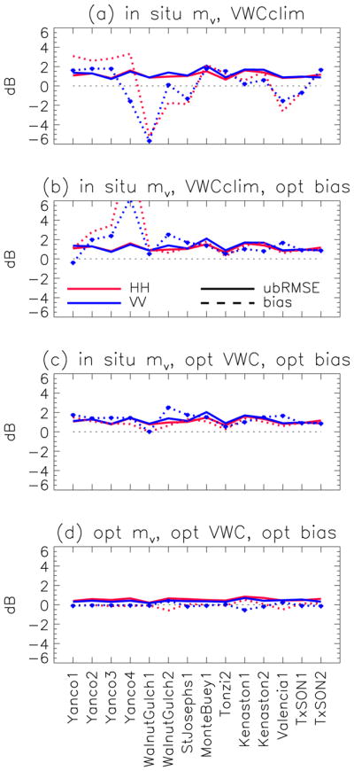
Forward model σ⁰ minus SMAP σ⁰ in dB, shown in terms of mean difference (dashed lines) and ubRMSE (solid lines) per each CVS. m_v denotes soil moisture. opt stands for “optimization” and is the derived value by the soil moisture retrieval process [defined in (1)]. VWCclim is the VWC climatology. Optimized values of soil moisture, VWC, and bias correspond to $\overline{m_{\upsilon }}$, f̄VWC, and c̄ in (1). (a) Model σ⁰ is computed using in situ m_v and VWCclim. (b) Model σ⁰ using in situ m_v, VWCclim, and optimized bias. (c) Model σ⁰ using in situ m_v, optimized VWC, and optimized bias. (d) Model σ⁰ using optimized m_v, optimized VWC, and optimized bias.

$$\begin{gathered} C(\overline{s},{\overline{\epsilon }}_{r1},{\overline{\epsilon }}_{r2},\dots ,{\overline{\epsilon }}_{rN}) \\ =w_{1,HH}{\left({\sigma }_{HH,1}^0-{\sigma }_{HH,\mathit{fwd}}^0(\overline{s},{\overline{\epsilon }}_{r1},\overline{f}{\mathit{VMC}}_1)+\overline{c}\right)}^2 \\ +w_{1,VV}{\left({\sigma }_{VV,1}^0-{\sigma }_{VV,\mathit{fwd}}^0(\overline{s},{\overline{\epsilon }}_{r1},\overline{f}{\mathit{VMC}}_1)+\overline{c}\right)}^2 \\ +w_{2,HH}{\left({\sigma }_{HH,2}^0-{\sigma }_{HH,\mathit{fwd}}^0(\overline{s},{\overline{\epsilon }}_{r2},\overline{f}{\mathit{VMC}}_2)+\overline{c}\right)}^2 \\ +w_{2,VV}{\left({\sigma }_{VV,2}^0-{\sigma }_{VV,\mathit{fwd}}^0(\overline{s},{\overline{\epsilon }}_{r2},\overline{f}{\mathit{VMC}}_2)+\overline{c}\right)}^2 \\ +\cdots +w_{N,HH}{\left({\sigma }_{HH,N}^0-{\sigma }_{HH,\mathit{fwd}}^0(\overline{s},{\overline{\epsilon }}_{rN},\overline{f}{\mathit{VMC}}_N)+\overline{c}\right)}^2 \\ +w_{N,VV}{\left({\sigma }_{VV,N}^0-{\sigma }_{VV,\mathit{fwd}}^0(\overline{s},{\overline{\epsilon }}_{rN},\overline{f}{\mathit{VMC}}_N)+\overline{c}\right)}^2 \end{gathered}$$ (1)

where the overbar denotes parameters that are retrieved. Numeric subscripts, 1, 2, …, N, are time indexes. Radar backscattering coefficients from observations and from the forward model are shown by σ⁰ and ${\sigma }_{\text{fwd}}^0$ (both in dB), respectively. s is the bare surface roughness, ε is the soil dielectric constant, w is the weight (uniform between channels and time instances because the error characteristics of σ⁰ are uniform across the channels; see [3, Appendix]). f is a retrieved factor for VWC adjustment, ranging from 0 to 2. c is a correction of any bias between measurement and model (physical sources of the bias in the forward model include missing physics such as the effect of topography, and mismatch of the number of discrete scatterers between nature and model). A dielectric model presented in [37] converts the estimated dielectric constants into soil moisture. To avoid an ill-posed retrieval, the number of unknowns should be less than the number of independent observations. The number of unknowns is N + 3, where N is the number of time-series instances and 3 corresponds to surface roughness, vegetation scaling factor, and bias. During the time period of N SMAP measurements, there are 2N copol observations (Table II), while the number of independent data could be 1.7N as estimated using the Aquarius radar data [38]. A minimum of N is deduced as 4.2 in order to facilitate a well-conditioned outcome. At least 16 temporal instances are available from SMAP data and are used in the retrieval. The surface roughness rms height is assumed to be constant during the time series; this assumption appears reasonable for regions without management activity and erosion. Management activity is rare in natural lands. Erosion becomes weak with vegetation canopy presence. The assumption would contribute to retrieval errors in regions with significant changes in surface roughness (e.g., in croplands) over the course of the time series. Directional roughness rms height was characterized for croplands at the field scale (e.g., [39]). At the 3-km scale, however, the directionality is expected to average out, and is not considered in this study.

TABLE II.

Examination of a Well-Constrained Retrieval Condition. N Is the Number of Time-Series Instances. N Is Larger than 16 for All CVS

Number of independent observation	2N
Number of free parameters	N+3

The retrieval is implemented as detailed in the SMAP Algorithm Theoretical Basis Document (ATBD) [39] and its flowchart is shown in Fig. 2. Time-series records of HH and VV are prepared and used as input to the retrieval. For each CVS site, a dominant type of vegetation is identified by referring to the landcover fraction derived with landcover databases (annual for U.S. and Canadian crops and climatology otherwise; see the ATBD for the complete list of landcover and crop-cover databases) and a local survey provided by CVS hosts (Table I). Accordingly, the forward models (datacubes) are selected for the CVS and are inverted in the retrieval. At a given set of candidate f and c, the optimizer searches ε and s; the search repeats for every candidate of f and c, and find the set of f, c, ε and s that gives minimum cost; the set becomes a final retrieval output. To create a global map of retrievals, the dielectric constant estimates at individual pixels are assembled. Finally, these are converted into soil moisture using the dielectric model [37].

Fig. 2.

Flowchart of algorithm.

Within St. Josephs site, corn occupied a smaller area than soybeans, but the corn σ⁰ can be four times (6 dB) larger than the soybean σ⁰ (see [1, Fig. 5]). The polarimetric signature also resembles that of the corn σ⁰ (see Section V), so that corn is selected to represent the St. Joseph’s site. The dominant landcover of the Kenaston site is wheat and lentils. In the absence of a lentils datacube, a wheat datacube is chosen because they both have a dominant vertical stem. Lentils have more leaves but L-band radar backscatter is relatively insensitive to thin leaves. For Valencia, the dominant landcover is vineyard, yet a vineyard datacube is not available. Alternatively, a corn datacube was used after noting that the observed polarimetric signature from the site shows an HH larger than VV (see Section V), which could occur when strong double-bounce is generated by the vertical trunks of grapevines. The simple and generally applicable rule based on the polarimetric property was effective in revising the cropcover classification for the crop CVS sites.

IV. Forward Model Evaluation

The forward models were trained using the measurements over land surfaces that do not have topography, subpixel heterogeneity in vegetation, azimuth anisotropy, and periodic row structure of crop fields. In contrast, these features of land surfaces are present within 3-km SMAP pixels on the global terrain. The first task of this section is to quantify the differences between the forward models and the SMAP observations of σ⁰ in the presence of these features. The second task is to demonstrate how the differences between the model and data are minimized through the optimization of (1) during the soil moisture retrieval. The physically based forward model requires three input parameters to predict σ⁰: soil moisture, surface roughness, and VWC. Ground truth information on these parameters at the CVS is currently available only for soil moisture. Ancillary VWC information is derived from a climatological VWC model. A first evaluation of the forward model is performed with the least number of optimized parameters

$${\sigma }_{\text{fwd}}^0=F(m_{\upsilon ,in\mathit{situ}},\overline{s},{\text{VWC}}_{\text{clim}})$$ (2)

where F denotes the forward model, m_{υ,in situ} is in situ soil moisture, and VWC_clim is the VWC climatology. Characterizations of surface roughness over a 3-km area are also not available from the CVS, so that retrieved roughness is used (s̄). After the optimization the forward model σ° may be written as

$${\sigma }_{\text{fwd}}^0=F(\overline{m_{\upsilon }},\overline{s},\overline{f}\times {\text{VWC}}_{\text{clim}},\overline{c})$$ (3)

where $\overline{m_{\upsilon }}$ is the retrieved soil moisture, f̄ is the retrieved scaling factor, and c̄ is the retrieved correction of bias in σ⁰.

Before optimization, the discrepancy between the SMAP observation and the forward model prediction is somewhat large. The standard deviation [equals the unbiased root-mean-squared error (ubRMSE)] of the difference is 1.2 dB for both the polarizations when averaged over the 14 CVS, with the averaged bias smaller than 0.5 dB [Fig. 3(a)]. Some of the large bias are analyzed below. The differences are within the range of the previous results. When the model σ⁰ was compared with the 80-km resolution spaceborne Aquarius observations (see [25, Fig. 8]) over homogeneous landcover and small terrain slope, they agreed with a mean difference of 2 dB over vegetated nonforest areas globally. The standard deviation of the difference between simulation and observation is about 2.5 dB (noncrop fields) and 4 dB (cropland and bare soil). This result suggests that the current evaluation is within expectation, since the spatial characteristics of σ⁰ is likely to be scalable over homogeneous flat natural terrains.

These σ⁰ differences before the optimization are significantly reduced as the bias, VWC, and soil moisture are optimized during the retrieval [Fig. 3(b)–(d)]. Eventually, the average of the difference over the 14 CVS are 0.5 dB (ubRMSE) and within −0.05 dB (bias) for both the polarizations [Fig. 3(d)]. The following error definitions are used [41]:

$$\begin{gathered} {(\text{ubRMSE})}^2=\frac{{(\mathrm{\Delta }(t)-\mathrm{\Delta })}^2}{N} \\ \text{bias}=\mathrm{\Delta }=\frac{\mathrm{\Delta }(t)}{N},{(\text{RMSE})}^2=\frac{{(\mathrm{\Delta }(t))}^2}{N} \end{gathered}$$ (4)

for the unbiased rms error, bias, and rms error, respectively, and where and N is number of time series inputs. For soil moisture, ubRMSE is more relevant than RMSE when retrieved soil moisture is assimilated into land surface or coupled models because a bias is removed before assimilation. An overview of the interpretation of the comparison results is presented below.

1. Terrain Slope: The large bias at Walnut Gulch1 before the optimization [Fig. 3(a)] is most likely associated with local topography. An elevation difference from ridge to valley is roughly 25 m over ground distances of around 170 m. While the site is located on hilly terrain, the forward model does not simulate how σ⁰ varies on a slope as the local incidence angle changes. A hill slope toward SMAP would generate a larger σ⁰ return. Consequently, the negative bias is expected as shown in Fig. 3(a). This bias is largely removed by the bias correction procedure [compare Fig. 3(a) and (b)]. The hills of Walnut Gulch2 are gentler than in Walnut Gulch1, which may explain the smaller bias in site 2. The size of the bias is similar between HH and VV. This is consistent with the airborne SAR observation where HH and VV showed a similar amount of change in response to the local incidence angle variations between 25° and 55° over a wide range of soil moisture conditions and vegetation types of grass, pasture, oat, and corn (see [42, Fig. 3]). The comparable size of bias between HH and VV supports the formulation in (1) that one correction factor is used for HH and VV.

2. Crop Row Structure: Anisotropic periodic structures on ground may explain the large ubRMSE found in Monte Buey [Fig. 3(a)]. This site consists of flat agricultural fields with uniform row directions in each field (Fig. 4). Seeding and harvesting were performed in the directions of field boundaries to allow tractor movements. These practices produced periodic row structures, which the forward model does not simulate. The structures were formed by the plants because there was no tillage. The SMAP σ⁰ is modulated by these structures, because SMAP’s azimuth viewing angle with respect to the row direction on the ground has six preferred values per 8-day repeat cycle (Fig. 4). For example, near the location at 500-km distance from nadir, the azimuth angle is almost perpendicular to the spacecraft velocity vector; while at 200-km from nadir, the angle is ~20° (fore-scan) and ~160° (aft-scan). The temporal fluctuations are found in SMAP real aperture (at 36 km) and SAR (1-km resolution) observations, suggesting that the fluctuations are caused by the widespread periodic structures on the ground.

3. VWC Climatology: The VWC input to the forward model calculation is initially the daily climatology based on the optical normalized difference vegetation index. Its scaling factor (f̄) is optimized to better represent the contemporary VWC. The VWC was modified in eight locations [Monte Buey, Yanco 1–4, Walnut Gulch1, St. Josephs, and Kenaston2 (see Figs. 4 and 5)]. The impact of revising VWC is shown most clearly in reducing the bias difference in the Yanco 3–4 sites [compare Fig. 3(b) and (c)].

4. Subpixel Heterogeneity and Fidelity of Scattering Model: Only one vegetation type of a forward model applies to a 3-km SMAP pixel during soil moisture retrieval, which implies that the soil moisture retrieval intrinsically assumes that the pixel is homogeneous. Except for the Monte Buey and Walnut Gulch1 sites, heterogeneous vegetation types are present within a 3-km pixel (Table I). Neglect of heterogeneity is expected to contribute to the differences in σ° in Fig. 3. The contribution will become greater as σ⁰ within a 3-km associated with different vegetation types becomes more heterogeneous (e.g., grass versus woody savanna in TxSON1, or bean and corn in St. Josephs). This effect is, however, reduced at Kenaston because of the structural similarity of different vegetation types and low crop developments during most of the observation period. The heterogeneity problem may be regarded as a part of the broader deficiency in scattering modeling. The deficiency is expected, because the models were trained over well-controlled homogeneous fields. The adjustment of soil moisture corrects for the deficiency in the forward model, as shown by the reduction in the σ⁰ difference [compare Fig. 3(c) and (d)]. Alternative approaches to resolve the heterogeneity are to premix the datacubes according to the subpixel fraction of landcover, or to perform retrieval at finer resolution and average to 3 km. These approaches significantly increase the computing requirements to perform global retrievals, but may be explored in the future.

In summary, the forward model and SMAP observations agree within 0.5 dB (ubRMSE) and −0.05 dB (bias) for both the polarizations [Fig. 3(d)]. These performance figures of the forward model are comparable with the prelaunch error budget designed to support soil moisture retrieval with an uncertainty of 0.06 m³/m³. In the prelaunch error budget (see [40], [25, Fig. 10]), a 0.7 dB (1σ) uncertainty in σ⁰ that was defined for the fore-and-aft scan averages of SMAP observations [42] ensued the soil moisture retrieval errors of smaller than 0.06 m³/m³ for nonforest landcover classes based on the Monte Carlo analysis. Based on these encouraging agreements, we will present the soil moisture retrieval results at the 14 CVS in the following section.

V. Soil Moisture Retrieval

The time-series comparisons of SMAP retrievals and upscaled averages of in situ measurements for the 3-km pixels at the CVS are presented in Figs. 4–6, and the statistics are summarized in Table III. Generally, good agreement is observed between the in situ and SMAP retrievals over diverse types of land and crop covers, but occasional large differences are found. Examples for specific sites are as follows.

TABLE III.

Validation of Retrievals at 13 Core Validation Sites Performed Over the 2.5-Month Period in 2015. R Refers to Pearson Correlation. (*) In Walnut Gulch, the Temporal Variation in In Situ Soil Moisture Is Very Small, Leading to the Negative or No Correlation

(m3/m3)	ubRMSE	Bias	RMSE	R
Cropland
St. Josephs1	0.051	−0.044	0.068	0.50
Kenaston1	0.104	−0.025	0.107	0.40
Kenaston2	0.087	−0.037	0.094	0.27
Monte Buey1	0.08	−0.016	0.082	0.59
Valencia1	0.032	0.026	0.041	0.42
Yanco1	0.049	−0.02	0.053	0.83
Crop Average	0.067	−0.019	0.074	0.50
Grassland
Walnut Gylch1	0.014	0.024	0.028	−0.47*
TxSON1	0.047	−0.038	0.060	0.80
TxSON2	0.053	−0.029	0.060	0.72
Tanco2	0.058	−0.013	0.059	0.75
Tanco3	0.040	−0.017	0.069	0.81
Tanco4	0.063	−0.008	0.063	0.52
Shrubland
Walnut Gulch2	0.017	−0.013	0.022	0.08*
Woody Savanna
Tonzi2	0.030	0.002	0.030	0.853
Non–crop Average	0.040	−0.012	0.054	0.51
All Site Average	0.052	−0.015	0.062	0.50

The Monte Buey site is a cropland with mostly soybeans in central Argentina. The large fluctuations in the retrievals are most likely caused by the periodic row structures of vegetation modulating σ° (Fig. 4, see the detailed discussion in Section IV), because the forward model does not yet incorporate the effects of row structures. After day 160 (June 9), the retrieval becomes too dry. This pattern in soil moisture is a response to the similar trend in σ⁰, suggesting that the dry bias is not an algorithm issue. Instead, this is expected because the harvest ended around day 153 with surface roughness having changed during the harvest. The optimized VWC of ~0.1 kg/m² is much smaller than the climatology of ~1 kg/m², but is consistent with dry vegetation during the senescence stage and with plant residues after harvest. As a separate experiment, soil moisture, VWC, and surface roughness were optimized during this postharvest period. The bias in estimated soil moisture of the postharvest period improved from −0.158 to −0.054 m³/m³. The surface roughness increased (from 2.15 to 2.47 cm) and VWC is reduced (VWC factor, f, changing from 0.3 to 0.05), which are consistent with the post-harvest conditions.

The Kenaston sites are in the Canadian prairies where wheat and lentils were seeded around the end of May (day 153). Kenaston2 has more lentils than winter wheat (Table I). A lentil plant resembles wheat or soybean structurally. Lentils have more leaves than wheats do but L-band radar backscattering is relatively insensitive to thin leaves. A wheat datacube was used for both the sites. Both the Kenaston sites show the large retrieval anomalies on day 126 (May 6), 162 (June 11), and 185/186 (July 4/5): these are responses to the anomalous σ⁰ (Fig. 5). These anomalies are coincident with light precipitation shown in the figure. When the rainfall is light and moistens only the surface soil, there can be difference between in situ (measured at 5-cm depth with the horizontally placed probes) and the L-band remote sensing (typically penetrating a few centimeters deep, but less when the soil is wet). Another possibility is the light rain wetting only the vegetation but not soil. However, the film of rain on the vegetation surface will be much thinner than leaf. A leaf with fluid inside does not contribute significantly to L-band backscattering, and even more so the thin rain film would do. When the roughness and soil moisture are retrieved after excluding the anomalous σ⁰, the ubRMSE of Kenaston1 improves to 0.060 m³/m³ with a correlation of 0.57 (from 0.102 m³/m³ and 0.40, respectively in Fig. 5 and Table IV); for Kenaston2, they improve to 0.058 m³/m³ and 0.64 (from 0.087 m³/m³ and 0.27).

TABLE IV.

Improved Retrieval After Excluding INPUT σ° That Are Spurious Due to the Light-Rain Effect. ubRMSE Is in m³/m³

	Kenaston 1		Kenaston 2		Yanco 4
	ubRMSE	correlation	ubRMSE	correlation	ubRMSE	correlation
Included	0.104	0.40	0.087	0.27	0.063	0.52
Excleded	0.060	0.57	0.058	0.64	0.033	0.89

The Yanco sites are located in the semiarid climate zone with little topography in Southwest Australia. Dominant land-cover types are pasture and wheat crops (Table I). In the Yanco 1–3 sites [44], the retrievals follow in situ data well with a ubRMSE smaller than 0.06 m³/m³. Optimized VWC is lower than the climatology, which is realistic considering that a pasture field in the semiarid area does not support the 1 kg/m² level of VWC [45] and the wheat seeded in early May reached only 10 cm height at the end of June (day 181). Some of the retrieval errors are examined as follows.

1. The retrievals have a dry bias after day 167 in Yanco1. Wheat crops that occupied ~90% of the area were seeded in May and grew from mid-June (day 166). Correspondingly, VWC should differ before and after around day 166, which is not correctly represented by the optimized VWC (green dots in Fig. 5). The misrepresentation and incomplete correction of the vegetation effect are likely one of the main causes of the dry bias.

2. At Yanco1, 2, and 4, anomalously wet retrievals were found on day 130 and 155 for Yanco 1 and 2, and day 139 and 155 for Yanco 4. These are responses to the anomalously high σ⁰. Any effect by periodic structures on the ground would be persistent in time as in the Monte Buey case, which is not the case here. These are attributed to the difference in sensing depth between radar and in situ probes in the presence of light rain, as explained in detail for the Kenaston sites. In Yanco, the in situ probes were placed vertically and measured soil moisture of top 5 cm, which, however, would not prevent the sensing depth discrepancy. Unfortunately, there is no concurrent precipitation data at the Yanco sites to confirm the causality.

3. The dry bias after day 167 is influenced by the anomalous σ⁰ on day 139 and 155, which alters the roughness estimate. When the roughness is retrieved after excluding the anomalous σ⁰, both of the ubRMSE and bias improve to 0.033 m³/m³ with correlation of 0.89 (from 0.063 m³/m³ and 0.52, respectively in Fig. 5 and Table IV).

4. At Yanco 1, the estimated roughness of 3.7 cm is large while the retrieved VWC is small at ~0.2 kg/m². These estimates are consistent with the field knowledge. In situ VWC was at about 0.2 kg/m² and soil was rough with furrows due to tillage. The tillage and seeding were completed toward the end of April. Until early July, the ground was covered by bare soil, 10-cm tall wheat, stubbles, and 20-cm tall pasture.

The Walnut Gulch sites are arid grassland and shrubland in Arizona, USA. During the SMAP radar period, the soil stayed dry at the residual level until it rained during late June when the monsoon began (Fig. 5). As a result of the small temporal variability, the ubRMSE of soil moisture retrieval of both the sites are very small (Table III). For the same reason, the correlation between in situ and retrieval is misleadingly low.

St. Josephs is an agricultural landscape in Indiana, USA. The 3-km pixel was covered approximately 44% by soybean and 38% by corn according to the local survey. Although the optimized cost [C in (1)] is similar between soybean and corn datacubes when each of them is used for retrieval, the ubRMSE of soil moisture retrieval is a factor of two smaller with the corn datacube. Corn’s acreage is smaller than that of soybean within the 3-km pixel, but corn σ⁰ can be 6 dB (four times) higher than soybean’s (see [1, Fig. 5]). Then the small areal fraction of corn can dominate σ⁰ of a heterogeneous pixel. The following observations support the hypothesis that the 3-km σ⁰ may be representing corn. The observed SMAP HH is often larger than VV (Fig. 5). Furthermore, soybean VWC does not reach beyond 1.5 kg/m², while the VWC at St. Josephs ranges from 1.5 to 4 kg/m²—the values for growing corn. Lastly, St. Josephs σ⁰ values are ~3 dB larger than Monte Buey σ⁰ where the landcover is 100% soybean.

Valencia site in Spain is covered mostly by vineyards (around 43%) with a fraction of natural vegetation (Mediterranean forests, matorral, and shrubs) of around 34%, urban and bare soil to about 6%, and other types of orchard trees (around 17%). However, a vineyard datacube is not available. As an alternative, the corn datacube is used after noting that the observed polarimetric properties show HH larger than VV. Physically, a grapevine has a prominent vertical trunk that is likely to scatter like a corn stalk.

TxSON is a rangeland located in central Texas, USA, on relatively flat terrain. During the period of data availability there were several rainfall events followed by dry downs. The climatology VWC of ~1 kg/m² is realistic for savanna grassland with scattered trees in a semiarid climate. Random grazing by livestock is not expected to produce temporal changes in the surface roughness. The large dynamic range of soil moisture is well described by the retrievals.

Tonzi is woody savanna in California. HH being larger than VV is perceived to be the double-bounce scattering from trees, which is confirmed by the analysis of scattering mechanism in Fig. 7. The amount of vegetation is the largest of all the CVS sites due to standing trees. Even in this relatively high biomass conditions, wetting and gradual dry downs are correctly monitored by the retrievals.

Fig. 7.

Scattering mechanisms shown by the forward models. The abscissa is the day of year in 2015 and the ordinate is in dB. The forward model σ⁰ is sampled with the retrievals of soil moisture, surface roughness, and vegetation water content.

The retrievals discussed above were performed using automated procedures (when choosing datacubes by referring to landcover database and when performing optimization) with a minimal amount of manual adjustment, so that the method may be applied globally over a long period of time. One of the exceptions to this strategy is the choice of the input ratio of correlation length to surface roughness (cl/s). Since CVS measurements do not provide the values of cl/s, a single number of 10 is used as an initial input for noncorn types (cl/s is difficult to characterize using measurements at 3-km scale). In the corn retrievals, σ⁰ is fairly independent of the ratio under the strong double-bounce conditions [22] and datacubes were generated with cl/s of 15 only. An exception is at TxSON2: the best retrieval was achieved with cl/s of 4. In the bare surface analysis, the retrieval was found insensitive to cl/s (see [3, Table III]), because different choices of cl/s added a quasi-bias and did not alter where the minimum of the cost function occurs (the location of the minimum is the retrieved soil moisture). In the CVS analysis, however, the sensitivity of soil moisture retrieval to cl/s is not fully understood. Over the cl/s range of 4 to 30, soil moisture retrieval was unaffected in terms of ubRMSE between 0.039 and 0.044 m³/m³ in the Yanco3 grassland; however, ubRMSE varied from 0.053 and 0.113 m³/m³ in the TxSON2 grassland.

The use of the physically based forward model provides an insight into the scattering mechanisms. The scattering mechanism is analyzed for Yanco2, Yanco3, Monte Buey, Tonzi, Kenaston2, and TxSON2 sites only, because the bias correction of these sites is sufficiently small (1 dB). The size of the bias correction has to be small, otherwise it will not be obvious to which of the three scattering mechanisms the bias can be attributed. In the two Yanco pasture fields, the surface scattering is dominant. σ⁰ of TxSON pasture fields is larger than Yanco values by more than 3 dB: surface scattering was similar between the TxSON and Yanco fields, but vegetation components explained most of the differences between the two locations. TxSON sites have sizeable fraction of trees (Table I), which contributes to the large scattering from vegetation. Scattering mechanism of the Monte Buey bean fields is similar to the Yanco pasture fields, where the surface scattering dominated. This similarity results from the fact that σ⁰ of the bean field was as small as the Yanco pasture fields. The optimized VWC of the Monte Buey site is as small as 0.2 kg/m² or lower, which is the vegetation amount of pasture fields, leading to the small σ⁰ of the bean field. Kenaston site is covered by wheat crops. The wheat stalk and leaf are so thin that their volume scattering is negligible, but the double bounce scattering from the vertical stalks become significant as the vegetation grows. Tonzi woody savanna case shows strong double bounce contributions from tree trunks. Even if the surface scattering is similar to those of the other fields, the double bounce is by far dominant.

In Summary, for the 14 CVS data sets, wetting and dry downs are well captured by the retrieval, with an overall correlation coefficient of 0.50 and a ubRMSE of 0.052 m³/m³, which meets the self-imposed target of 0.06 m³/m³ [40]. Generally, the statistics for noncroplands are better than those of croplands (ubRMSE of 0.040 versus 0.067 m³/m³ Fig. 6 and Table III). Croplands pose more challenges as discussed above, notably temporal changes in vegetation and surface roughness, periodic row structures, and a diversity of crop types that produce distinctively different scattering mechanisms. Some of the differences in the CVS comparisons may be generated by nonalgorithmic caused such as the discrepancy in sensing depth of radar versus in situ sensors. Excluding these cases, the ubRMSE improves by nearly a factor of two (Table IV) on each CVS and, since these cases occur on as many as five CVS, the overall ubRMSE is expected to improve. The correlation could improve as well if the arid Walnut Gulch comparisons are excluded, where the correlation has little meaning when soil moisture varied little in time.

VI. Conclusion

SAR-based soil moisture retrieval over diverse conditions of soil moisture, surface roughness, and vegetation on a global basis has rarely been performed due to the lack of data and difficulty of performing robust and reliable retrievals. To account for significantly different mechanisms of radar response to soil moisture among vegetation types, the forward models (datacubes) were developed for each of 12 landcover classes. The unknown surface roughness is estimated and constrained using the time-series approach. The estimated roughness is within the expectation of 0.5–4 cm. The ill-posed retrieval conditions are mitigated by incorporating the dual-copolarization SAR inputs (Table II). While the algorithms were tested previously over homogeneous field campaign sites, the current results are the tests over challenges in the global 3-km SMAP data including periodic ground structure of croplands, temporal changes in VWC, terrain slope, and subpixel heterogeneity.

Before the optimization of the retrieval process, the forward model had somewhat large differences from the observed SMAP σ⁰, most likely because of deficiencies in accounting for the effects of terrain slope, unknown correlation length of surface roughness, periodic structure of croplands, uncertainty in vegetation input, and subpixel heterogeneity [Fig. 3(a)]. After the optimization, the difference over the 14 core validation sites (CVS) is reduced to 0.5 dB (ubRMSE) and within −0.05 dB (bias) for both the polarizations [Fig. 3(d)]. This level of agreement is comparable with the prelaunch error budget to support soil moisture retrieval with an uncertainty target of 0.06 m³/m³.

The soil moisture retrievals were assessed at the rigorously selected 14 CVS covering a range of vegetation types that included grass, pasture, shrub, corn, wheat, bean, and woody savanna around the world from mid-April to early July 2015. The ubRMSE of soil moisture retrieval is found to be 0.052 m³/m³, which meets the accuracy target (see Figs. 4 and 5, and Table III). The difference over croplands is larger than those of noncroplands (see Fig. 6 and Table III), which is anticipated because of the complexities of the cropland such as periodic structure on the ground, temporal changes in surface roughness due to tilling operations, temporal changes in VWC, and subpixel heterogeneity. The retrievals were performed by automated procedures with a minimal amount of manual adjustment, so that the method may be applied globally and operationally. The anomalous retrievals might have occurred when the sensing depth differs between SMAP radar and in situ sensors. Excluding these cases manually, the ubRMSE of the affected CVS improves by a factor of two (Table IV), and the overall ubRMSE is expected to improve accordingly.

Biographies

Seung-Bum Kim received the B.Sc. degree in electrical engineering from the Korea Advanced Institute of Science and Technology, Daejeon, South Korea, in 1992, and the M.S. and Ph.D. degrees in remote sensing from University College London, London, U.K., in 1993, and 1998, respectively.

He was a Scientist at Remote Sensing Systems, Santa Rosa, CA, USA, studying the L-band radiometry for the Aquarius salinity observation. He has been with the Jet Propulsion Laboratory, Pasadena, CA, USA, since 2009. His current research interests include microwave modeling, soil moisture retrieval with the radar data from the Soil Moisture Active Passive (SMAP) mission, and salinity retrieval with the Aquarius data.

Dr. Kim is a member of the Aquarius and SMAP science teams. He was a recipient of the Best Paper Awards from the U.K. and Korean remote sensing societies, and the NASA group achievement awards.

Jakob J. van Zyl, (F’99) photograph and biography not available at the time of publication.

Joel T. Johnson (S’88–M’96–SM’03–F’08) received the bachelor’s degree in electrical engineering from the Georgia Institute of Technology, Atlanta, GA, USA, in 1991, and the S.M. and Ph.D. degrees from the Massachusetts Institute of Technology, Cambridge, MA, USA, in 1993 and 1996, respectively.

He is currently a Professor and Chair with the Department of Electrical and Computer Engineering and ElectroScience Laboratory, The Ohio State University, Columbus, OH, USA. His current research interests include microwave remote sensing, propagation, and electromagnetic wave theory.

Dr. Johnson is a member of the Commissions B and F of the International Union of Radio Science (URSI), and a member of Tau Beta Pi, Eta Kappa Nu, and Phi Kappa Phi. He was a recipient of the 1993 Best Paper Award from the IEEE Geoscience and Remote Sensing Society, was named an Office of Naval Research Young Investigator, National Science Foundation Career Award, received the PECASE Award in 1997, and was recognized by the U.S. National Committee of URSI as a Booker Fellow in 2002.

Matha Moghaddam (S’86–M’87–SM’02–F’08) received the B.S. (Hons.) degree in electrical and computer engineering from the University of Kansas, Lawrence, KS, USA, in 1986, and the M.S. and Ph.D. degrees in electrical and computer engineering from the University of Illinois at Urbana–Champaign, Champaign, IL, USA, in 1989 and 1991, respectively.

From 1991 to 2003, she was with the NASA Jet Propulsion Laboratory (JPL), Pasadena, CA, USA, and from 2003 to 2011, she was with the University of Michigan, Ann Arbor, MI, USA. She has introduced new approaches for quantitative interpretation of multichannel radar imagery based on analytical inverse scattering techniques applied to complex and random media. She was a Systems Engineer for the Cassini Radar and served as the Science Chair of the JPL Team X (Advanced Mission Studies Team). She is currently a Professor of Electrical Engineering with the University of Southern California, Los Angeles, CA, USA. Her current research interests include the development of new radar instrument and measurement technologies for subsurface and subcanopy characterization, development of forward and inverse scattering techniques for layered random media especially for soil moisture applications, and transforming concepts of radar remote sensing to near-field and medical imaging.

Dr. Moghaddam is a member of the Soil Moisture Active and Passive mission Science Team, and the Principal Investigator of the AirMOSS NASA Earth Ventures 1 mission. She is the Editor-in-Chief of the IEEE Antennas and Propagation Magazine.

Leung Tsang (F’90–LF’16) was born in Hong Kong. He received the S.B., S.M., and Ph.D. degrees from the Department of Electrical Engineering and Computer Science, Massachusetts Institute of Technology, Cambridge, MA, USA.

He was the Chair of the Department of Electronic Engineering, City University of Hong Kong, Hong Kong, from 2006 to 2011. Between 2001 and 2004, he was on leave with the department. Since 1983, he has been with the University of Washington, Seattle, WA, USA, where he is currently a Professor of Electrical Engineering. He is the lead author of four books titled Theory of Microwave Remote Sensing and Scattering of Electromagnetic Waves (Volumes 1, 2, and 3). His current research interests include waves in random media, remote sensing and geoscience applications, computational electromagnetics, and signal integrity and optic.

Dr. Tsang has been a member of the Washington State Academy of Sciences since 2012. He is a fellow of the Optical Society of America. He was a recipient of the IEEE Third Millennium Medal and the Outstanding Service Award from the IEEE Geoscience and Remote Sensing Society in 2000, the Distinguished Achievement Award from the IEEE Geoscience and Remote Sensing Society in 2008, the Fiorino Oro Award from the CeTeM, Italy, in 2010, the William Pecora Award co-sponsored by the U.S. Department of Interior and NASA in 2012, and the 2013 IEEE Electromagnetics Award. He was the President of the IEEE Geoscience and Remote Sensing Society in 2006–2007, and the Editor-in-Chief of the IEEE Transactions on Geoscience and Remote Sensing in 1996–2001.

Andreas Colliander (S’04–A’06–M’07–SM’08) received the M.Sc. (Tech.), Lic.Sc. (Tech.), and D.Sc. (Tech.) degrees from the Helsinki University of Technology (TKK; now Aalto University), Espoo, Finland, in 2002, 2005, and 2007, respectively.

He is currently a Research Scientist with the Jet Propulsion Laboratory, California Institute of Technology, Pasadena, CA, USA. He is a member of the Science Algorithm Development Team with the Soil Moisture Active and Passive mission, where he focuses on the calibration and validation of the geophysical products. He is also funded by NASA to study intercalibration of spaceborne radiometers, improve soil moisture retrieval algorithms, and develop long-term soil moisture records.

Roy Scott Dunbar received the B.S. degree in physics and astronomy from the University of Albany, Albany, NY, USA, in 1976, and the Ph.D. degree in physics from Princeton University, Princeton, NJ, USA, in 1980.

He has been with the Jet Propulsion Laboratory, Pasadena, CA, USA, since 1981. Over the last 30 years, he has contributed to the development of science algorithms for the NSCAT and SeaWinds ocean vector wind scatterometer projects, and since 2009, he has been involved in SMAP soil moisture and freeze–thaw algorithm development.

Thomas J. Jackson (SM’96–F’02) received the Ph.D. degree from the University of Maryland, College Park, MD, USA, in 1976.

He is currently a Research Hydrologist with the U.S. Department of Agriculture, Agricultural Research Service, Hydrology and Remote Sensing Laboratory, Beltsville, MD, USA. He is a member of the science and validation teams of the Aqua, ADEOS-II, Radarsat, Oceansat-1, Envisat, ALOS, SMOS, Aquarius, GCOM-W, and SMAP remote sensing satellites. His current research interests include the application and development of remote sensing technology in hydrology and agriculture, primarily microwave measurement of soil moisture.

Dr. Jackson is a fellow of the Society of Photo-Optical Instrumentation Engineers, the American Meteorological Society, and the American Geophysical Union. He was a recipient of the William T. Pecora Award (NASA and Department of Interior) for outstanding contributions toward understanding the Earth by means of remote sensing in 2003, the AGU Hydrologic Sciences Award for outstanding contributions to the science of hydrology, and the IEEE Geoscience and Remote Sensing Society Distinguished Achievement Award in 2011.

Sermsak Jaruwatanadilok (M’03) received the B.E. degree in telecommunication engineering from the King Mongkut’s Institute of Technology, Ladkrabang, Thailand, in 1994, the M.S. degree in electrical engineering from Texas A&M University, College Station, TX, USA, in 1997, and the Ph.D. degree in electrical engineering from the University of Washington, Seattle, WA, USA, in 2003.

From 2006 to 2010, he was a Research Assistant Professor with the University of Washington. He is currently a System Engineer with the Jet Propulsion Laboratory, California Institute of Technology, Pasadena, CA, USA. His current research interests include electromagnetic wave propagation in random and complex media and remote sensing.

Richard West received the Ph.D. degree in electrical engineering from the University of Washington, Seattle, WA, USA, in 1994. His Ph.D. dissertation applied dense medium scattering theory to the analysis of passive microwave measurements of Antarctic snow.

In 1995, he joined the Radar Science and Engineering section with the Jet Propulsion Laboratory, California Institute of Technology, Pasadena, CA, USA. He was involved in the development of algorithms for the processing and calibration of data from the NASA Scatterometer, and from SeaWinds on QuikScat. In 1999, he joined the radar instrument on the Cassini Mission to Saturn, and became the Deputy Task Manager in 2002. During the Cassini Mission, from 2004 to 2016, he was involved in all aspects of instrument operations including planning the science observations in coordination with the science team, designing the radar command sequences, and processing/calibrating the data received. From 2009 to 2016, he was involved in radar backscatter processing for the Soil Moisture Active/Passive project, and in 2016, he was with the NASA’s planned mission to Europa and the REASON radar sounder instrument. His current research interests include electromagnetic scattering theory, the applications of active and passive microwave data to problems in remote sensing and planetary science, and the development of new techniques/technology to enable more capable remote sensing missions.

Aaron Berg received the B.Sc. and M.Sc. degrees in geography from the University of Lethbridge, Lethbridge, AB, Canada, the M.S. degree in geological sciences from the University of Texas, Austin, TX, USA, and the Ph.D. degree in earth system science from the University of California, Irvine, CA, USA.

He is currently a Professor and Canada Research Chair in Hydrology and Remote Sensing with the Department of Geography, University of Guelph, Guelph, ON, Canada. He teaches Physical Geography, Hydrology, and Remote Sensing, with research interests in hydrological modeling and terrestrial remote sensing.

Todd Caldwell received the B.S. degree in earth and planetary sciences from the University of New Mexico, Albuquerque, NM, USA, in 1997, and the M.Sc. and Ph.D. degrees in hydrogeology from the University of Nevada, Reno, NV, USA, in 1999 and 2007, respectively.

Since 2012, he has been a Research Hydrologist and Geoscientist with the Bureau of Economic Geology, the Jackson School of Geosciences, University of Texas, Austin, TX, USA. From 2002 to 2012, he was a Research Soil Scientist with the Desert Research Institute, Reno. He is a Principle Investigator of the Texas Soil Observation Network and a SMAP core calibration and validation site. His current research interests include field investigations and modeling of soil and vadose zone processes across multiple scales and environments.

Michael H. Cosh (M’02) received the Ph.D. degree from Cornell University, Ithaca, NY, USA, in 2002.

He is a Research Hydrologist with the U.S. Department of Agriculture, Agricultural Research Service, Hydrology and Remote Sensing Laboratory, Beltsville, MD, USA. His current research interests include the monitoring of soil moisture from both in situ resources and satellite products.

Dr. Cosh is a member of the United States Department of Agriculture Remote Sensing Coordination Committee. He has served as the Chairperson of both the Remote Sensing Technical Committee and the Large Scale Field Experiments Technical Committee for the American Geophysical Union. He currently serves on the World Meteorological Organization’s Committee on Agricultural Meteorology-Soil Moisture.

David C. Goodrich received the Ph.D. degree from the Department of Hydrology and Water Resources, University of Arizona, Tuscon, AZ, USA, in 1990.

He held various positions with the U.S. Geological Survey, WI, USA, and AK, USA, and was a Consultant with Autometric, Washington, WA, USA. Since 1988, he has been a Research Hydraulic Engineer with the Southwest Watershed Research Center of the USDA Agricultural Research Service, Tucson. His current research interests include scaling issues in watershed rainfall-runoff response, identification of dominant hydrologic processes over a range of basin scales, climatic change impacts on semiarid hydrologic response, incorporation of remotely sensed data into hydrologic models, the functioning of semiarid riparian systems, nonmarket valuation of ecosystem services, flash-flood forecasting, and rapid post-fire watershed assessments. He co-led the interdisciplinary multiagency Semi-Arid Land-Surface-Atmosphere Research Program. He was an Executive Member of the National Science Foundation Sustainability of the Semi-Arid Hydrology and Riparian Areas Science and Technology Center and has been involved closely with elected officials and decision-makers at the San Pedro Basin since 2000.

Stanley Livingston received the B.S. degree in forestry and the M.S. degree in soil genesis from Purdue University, West Lafayette, IN, USA, in 1981 and 1990, respectively.

From 1981 to 1990, he was a Research Technician with the National Soil Erosion Research Laboratory, USDA-ARS, West Lafayette. From 1984 to 1987, and since 1990, he has been a support Soil Scientist at the National Soil Erosion Research Laboratory. Currently, he is involved in watershed water quality monitoring and BMP comparisons in the Western Lake Erie Basin at Northeast Indiana. The research focuses on field based water quality monitoring and innovative BMP’s for water quality remediation. His current research interests include blind inlet design and water discharge measurement techniques.

Ernesto López-Baeza received the Ph.D. degree in physics from the University of Valencia, Valencia, Spain, in 1986.

He has been an Associate Professor of Applied Physics with the University of Valencia since 1987, and has been the Director of the Climatology from Satellites Group since 2000. He is in charge of two surface validation facilities, namely, the Valencia and the Alacant Anchor Stations in Spain. His research interests included the ground validation activities in the framework of EUMETSAT Geostationary Earth Radiation Budget, NASA Clouds and the Earth’s Radiant Energy System, ESA/JAXA Earth Clouds, Aerosols and Radiation Explorer (EarthCARE), and ESA/EUMETSAT EPS/MetOp. He is currently involved in scientific activities of the Earth Observation missions: Soil Moisture Active and Passive from NASA, Soil Moisture and Ocean Salinity from ESA, and the Ocean and Land Color Instrument onboard Copernicus Sentinel-3 satellite. His current research interests include the validation of low-resolution remote sensing data and products.

Tracy Rowlandson received the B.Sc. degree in environmental science and the M.Sc. degree from the University of Guelph, Guelph, ON, Canada, in 2003 and 2006, respectively, and the Ph.D. degree in agricultural meteorology from the Department of Agronomy, Iowa State University, Ames, IA, USA, in 2011.

She is currently a Research Associate with the Department of Geography, University of Guelph. Her current research interests include investigating the impact of vegetation and soil management practices on soil moisture retrieval using passive and active microwave remote sensing.

Marc Thibeault received the B.Sc. degree in physics from Laval University, Québec, QC, Canada, in 1982, the B.Sc. degree in mathematics from the University of Montréal, Montréal, QC, in 1988, and the D.C. degree in science from the University of Buenos Aires, Buenos Aires, Argentina, in 2004.

He is currently a Strategic Applications Coordinator of the SAOCOM project, a new L-Band mission of the Argentinian Space Agency, Paseo Colón, Argentina. His current research interests include soil moisture, polarimetry, and other SAR applications.

Jeffrey P. Walker received the B.E. (civil) and B.Surveying degrees (with Hons. 1 and University Medal) and the Ph.D. degree in water resources engineering from the University of Newcastle, Callaghan, NSW, Australia, in 1995 and 1999, respectively. His Ph.D. dissertation was among the early pioneering research on estimation of root-zone soil moisture from assimilation of remotely sensed surface soil moisture observations.

He joined the NASA Goddard Space Flight Center, Greenbelt, MD, USA, to implement his soil moisture work globally. In 2001, he moved to the Department of Civil and Environmental Engineering, University of Melbourne, Melbourne, VIC, Australia, as a Lecturer, where he continued his soil moisture work, including the development of the only Australian airborne capability for simulating new satellite missions for soil moisture. In 2010, he became a Professor with the Department of Civil Engineering, Monash University, Melbourne, where he is continuing this research. He contributes to soil moisture satellite missions at NASA, ESA, and JAXA, as a Science Team Member for the Soil Moisture Active Passive mission and a Cal/val Team Member for the Soil Moisture and Ocean Salinity and Global Change Observation Mission-Water, respectively.

Dara Entekhabi (M’04–SM’09–F’15) received the B.S. and M.S. degrees from Clark University, Worcester, MA, USA, and the Ph.D. degree from the Massachusetts Institute of Technology (MIT), Cambridge, MA, USA, in 1990.

He is currently a Professor with the Department of Civil and Environmental Engineering and the Department of Earth, Atmospheric and Planetary Sciences, MIT. He is the Science Team Lead for the National Aeronautics and Space Administration’s Soil Moisture Active and Passive (SMAP) mission that was launched January 31, 2015. His research includes terrestrial remote sensing, data assimilation, and coupled land-atmosphere systems modeling.

Prof. Entekhabi is a Fellow of the American Meteorological Society and the American Geophysical Union.

Eni G. Njoku (M’75–SM’83–F’95) received the B.A. degree in natural and electrical sciences from Cambridge University, Cambridge, U.K., in 1972, and the M.S. and Ph.D. degrees in electrical engineering from the Massachusetts Institute of Technology, Cambridge, MA, USA, in 1974 and 1976, respectively.

He was a Senior Research Scientist with the Surface Hydrology Group at the Jet Propulsion Laboratory, California Institute of Technology, Pasadena, CA, USA, until his retirement in 2016. He was the Project Scientist of the Soil Moisture Active Passive mission from 2008 to 2013 and a member of the U.S. Advanced Microwave Scanning Radiometer science team. His current research interests include passive and active microwave sensing of soil moisture for hydrology and climate applications.

Dr. Njoku was a recipient of the NASA Exceptional Public Service Medal in 2016.

Peggy E. O’Neill (F’16) received the B.S. (summa cum laude) degree (with Hons.) in geography from Northern Illinois University, DeKalb, IL, USA, in 1976, and the M.A. degree in geography from the University of California, Santa Barbara, CA, USA, in 1979.

She has done post-graduate work in civil and environmental engineering with Cornell University, Ithaca, NY, USA. Since 1980, she has been a Physical Scientist with the Hydrological Sciences Laboratory at the NASA/Goddard Space Flight Center, Greenbelt, MD, USA, where she conducts research in soil moisture retrieval and land surface hydrology, primarily through microwave remote sensing techniques, and is currently the SMAP Deputy Project Scientist.

Simon H. Yueh (F’09) received the Ph.D. degree in electrical engineering in January 1991 from the Massachusetts Institute of Technology (MIT), Cam-bridge, MA, USA.

He was a Postdoctoral Research Associate at MIT from February to August 1991. In September 1991, he joined the Radar Science and Engineering Section, Jet Propulsion Laboratory (JPL). He was the Supervisor of the radar system engineering and algorithm development group from 2002–2007, the Deputy Manager of the Climate, Oceans and Solid Earth section from 2007–2009, and the Section Manager from 2009–2013. He has served as the Project Scientist of the National Aeronautics and Space Administration (NASA) Aquarius mission from January 2012 to September 2013, the Deputy Project Scientist of NASA’s Soil Moisture Active Passive Mission from January 2013 to September 2013, and the SMAP Project Scientist since October 2013. He has been the Principal/Co-Investigator of numerous NASA and Department of Defense research projects on remote sensing of soil moisture, terrestrial snow, ocean salinity, and ocean wind. He has authored four book chapters and published more than 150 publications and presentations.

Dr. Yueh received the IEEE Geoscience and Remote Sensing Society Transaction Prize Paper award in 1995, 2002, 2010, and 2014. He also received the 2000 Best Paper Award in the IEEE International Geoscience and Remote Sensing Symposium. He received the JPL Lew Allen Award in 1998 and Ed Stone Award in 2003. He received the NASA Exceptional Technology Achievement Medal in 2014. He is a member of URSI Commission-F and an Associate Editor of the IEEE Transcations on Geoscience and Remote Sensing.

References

- 1.McNairn H, et al. The soil moisture active passive validation experiment 2012 (SMAPVEX12): Prelaunch calibration and validation of the SMAP soil moisture algorithms. IEEE Trans Geosci Remote Sens. 2015 May;53(5):2784–2801. [Google Scholar]
- 2.Huang S, Tsang L, Njoku EG, Chen KS. Backscattering coefficients, coherent reflectivities, and emissivities of randomly rough soil surfaces at L-band for SMAP applications based on numerical solutions of Maxwell equations in three-dimensional simulations. IEEE Trans Geosci Remote Sens. 2010 Jun;48(6):2557–2568. [Google Scholar]
- 3.Kim S-B, Tsang L, Johnson JT, Huang S, van Zyl JJ, Njoku EG. Soil moisture retrieval using time-series radar observations over bare surfaces. IEEE Trans Geosci Remote Sens. 2012 May;50(5):1853–1863. [Google Scholar]
- 4.Balenzano A, Mattia F, Satalino G, Davidson MWJ. Dense temporal series of C- and L-band SAR data for soil moisture retrieval over agricultural crops. IEEE J Sel Topics Appl Earth Observ Remote Sens. 2011 Jun;4(2):439–440. [Google Scholar]
- 5.Ouellette JD, et al. A time-series approach to estimating soil moisture from vegetated surfaces using L-band radar backscatter. IEEE Trans Geosci Remote Sens. to be published. [Google Scholar]
- 6.Bindlish R, Jackson T, Sun R, Cosh M, Yueh S, Dinardo S. Combined passive and active microwave observations of soil moisture during CLASIC. IEEE Geosci Remote Sens Lett. 2009 Oct;6(4):644–648. [Google Scholar]
- 7.De Roo RD, Du Y, Dobson MC, Ulaby FT. A semi-empirical backscattering model at L-band and C-band for a soybean canopy with soil moisture inversion. IEEE Trans Geosci Remote Sens. 2001 Apr;39(4):864–872. [Google Scholar]
- 8.Joseph AT, van der Velde R, O’Neill PE, Lang RH, Gish T. Soil moisture retrieval during a corn growth cycle using L-band (1.6 GHz) radar observations. IEEE Trans Geosci Remote Sens. 2008 Aug;46(8):2365–2374. [Google Scholar]
- 9.Narvekar PS, Entekhabi D, Kim SB, Njoku EG. Soil moisture retrieval using L-band radar observations. IEEE Trans Geosci Remote Sens. 2015 Jun;53(6):3492–3506. [Google Scholar]
- 10.Pierdicca N, Pulvirenti L, Bignami C, Ticconi F. Monitoring soil moisture in an agricultural test site using SAR data: Design and test of a pre-operational procedure. IEEE J Sel Topics Appl Earth Observ Remote Sens. 2013 Jun;6(3):1199–1210. [Google Scholar]
- 11.Zribi M, Gorrab A, Baghdadi N. A new soil roughness parameter for the modelling of radar backscattering over bare soil. Remote Sens Environ. 2014;152:62–73. [Google Scholar]
- 12.Kim Y, van Zyl JJ. A time-series approach to estimate soil moisture using polarimetric radar data. IEEE Trans Geosci Remote Sens. 2009 Aug;47(8):2519–2527. [Google Scholar]
- 13.Naeimi V, Scipal K, Bartalis Z, Hasenauer S, Wagner W. An improved soil moisture retrieval algorithm for ERS and METOP scatterometer observations. IEEE Trans Geosci Remote Sens. 2009 Jul;47(7):1999–2013. [Google Scholar]
- 14.Ali I, Greifeneder F, Stamenkovic J, Neumann M, Notarnicola C. Review of machine learning approaches for biomass and soil moisture retrievals from remote sensing data. Remote Sens. 2015;12(7):16398–16421. [Google Scholar]
- 15.Frate FD, et al. Wheat cycle monitoring using radar data and a neural network trained by a model. IEEE Trans Geosci Remote Sens. 2004 Jan;42(1):35–44. [Google Scholar]
- 16.Paloscia S, Pampaloni P, Pettinato S, Santi E. A comparison of algorithms for retrieving soil moisture from ENVISAT/ASAR images. IEEE Trans Geosci Remote Sens. 2008 Oct;46(10):3274–3284. [Google Scholar]
- 17.Njoku EG, et al. Observations of soil moisture using a passive and active low-frequency microwave airborne sensor during SGP99. IEEE Trans Geosci Remote Sens. 2002 Dec;40(12):2659–2673. [Google Scholar]
- 18.Duan X, Moghaddam M. 3-D vector electromagnetic scattering from arbitrary random rough surfaces using stabilized extended boundary condition method for remote sensing of soil moisture. IEEE Trans Geosci Remote Sens. 2012 Jan;50(1):87–103. [Google Scholar]
- 19.Mcdonald KC, Dobson MC, Ulaby FT. Using mimics to model L-band multiangle and multitemporal backscatter from a walnut orchard. IEEE Trans Geosci Remote Sens. 1990 Jul;28(4):477–491. [Google Scholar]
- 20.Lang RH, Sighu JS. Electromagnetic backscattering from a layer of vegetation: A discrete approach. IEEE Trans Geosci Remote Sens. 1983 Jan;GE-21(1):62–71. [Google Scholar]
- 21.Huang H, et al. Coherent model of L-band radar scattering by soybean plants: Model development, evaluation, and retrieval. IEEE J Sel Topics Appl Earth Observ Remote Sens. 2016 Jan;9(1):272–284. doi: 10.1109/JSTARS.2015.2469717. [DOI] [Google Scholar]
- 22.Liao TH, Kim SB, Tan S, Tsang L, Su C, Jackson TJ. Multiple scattering effects with cyclical correction in active remote sensing of vegetated surface using vector radiative transfer theory. IEEE J Sel Topics Appl Earth Observ Remote Sens. 2016 Apr;9(4):1414–1429. doi: 10.1109/TGRS.2016.2517010. [DOI] [Google Scholar]
- 23.Bracaglia M, Ferrazzoli P, Guerriero L. A fully polarimetric multiple scattering model for crops. Remote Sens Environ. 1995;54(3):170–179. [Google Scholar]
- 24.Burgin M, Clewley D, Lucas RM, Moghaddam M. A generalized radar backscattering model based on wave theory for multilayer multispecies vegetation. IEEE Trans Geosci Remote Sens. 2011 Dec;49(12):4832–4845. [Google Scholar]
- 25.Kim SB, Moghaddam M, Tsang L, Burgin M, Xu X, Njoku EG. Models of L-band radar backscattering coefficients over global terrain for soil moisture retrieval. IEEE Trans Geosci Remote Sens. 2014 Feb;52(2):1381–1396. [Google Scholar]
- 26.Tabatabaeenejad A, Burgin M, Moghaddam M. Potential of L-band radar for retrieval of canopy and subcanopy parameters of boreal forests. IEEE Trans Geosci Remote Sens. 2012 Jun;50(6):2150–2160. [Google Scholar]
- 27.Akbar R, Moghaddam M. A combined active–passive soil moisture estimation algorithm with adaptive regularization in support of SMAP. IEEE Trans Geosci Remote Sens. 2015 Jun;53(6):3312–3324. [Google Scholar]
- 28.Entekhabi D, et al. The soil moisture active passive (SMAP) mission. Proc IEEE. 2010 May;98(5):704–716. [Google Scholar]
- 29.Pathe C, Wagner W, Sabel D, Doubkova M, Basara JB. Using ENVISAT ASAR global mode data for surface soil moisture retrieval over Oklahoma, USA. IEEE Trans Geosci Remote Sens. 2009 Feb;47(2):468–480. [Google Scholar]
- 30.Fore AG, et al. Aquarius scatterometer calibration. IEEE J Sel Topics Appl Earth Observ Remote Sens. 2015 Dec;8(12):5424–5432. [Google Scholar]
- 31.West R. Tech Rep D-98986. Jet Propuls. Lab; Pasadena, CA, USA: 2015. Soil moisture active passive (SMAP) project radar backscatter calibration for the L1B_S0_LoRes and L1C_S0_HiRes validated level data products. [Google Scholar]
- 32.Committee on Earth Observation Satellites (CEOS) Working Group on Calibration and Validation (WGCV) and Land Products SubGroup of Committee on Earth Observation Satellites (CEOS) Working Group on Calibration and Validation (WGCV) [Online]. Available: http://calvalportal.ceos.org and http://lpvs.gsfc.nasa.gov.
- 33.Famiglietti JS, Ryu D, Berg AA, Rodell M, Jackson TJ. Field observations of soil moisture variability across scales. Water Resour Res. 2008;44(1):W01423. [Google Scholar]
- 34.Colliander A. SMAP L2-L4 Data Product CalVal Plan, document JPL D-79463. Jet Propulsion Laboratory; Pasadena, CA, USA: 2014. p. 85. [Google Scholar]
- 35.Colliander A, et al. SMAP L2/L3 soil moisture product validation with core validation sites. Remote Sens Environ. to be published. [Google Scholar]
- 36.van Zyl J, Kim Y. Applications: Measurement of surface soil moisture. In: van Zyl JJ, Kim Y, editors. Synthetic Aperture Radar Polarimetry. Hoboken, NJ, USA: Wiley; 2011. p. 312. (JPL Space Science and Technology Series) [Google Scholar]
- 37.Mironov VL, Dobson MC, Kaupp VH, Komarov SA, Kleshchenko VN. Generalized refractive mixing dielectric model for moist soils. IEEE Trans Geosci Remote Sens. 2004 Apr;42(4):773–785. [Google Scholar]
- 38.Konings AG, McColl KA, Piles M, Entekhabi D. How many parameters can be maximally estimated from a set of measurements? IEEE Geosci Remote Sens Lett. 2015 May;12(5):1081–1085. [Google Scholar]
- 39.Marzahn P, Ludwig R. On the derivation of soil surface roughness from multi parametric PolSAR data and its potential for hydrological modeling. Hydrol Earth Syst Sci. 2009 Mar;13:381–394. [Google Scholar]
- 40.Kim SB, van Zyl JJ, Dunbar S, Johnson JT, Moghaddam M, Tsang L. Tech Rep. Jet Propuls. Lab; Pasadena, CA, USA: 2015. SMAP algorithm theoretical basis document: L2 & L3 radar soil moisture (active) products. Revision B; p. 56. [Online]. Available: http://nsidc.org/data/docs/daac/smap/sp_l2_sma/pdfs/L2&3_SM_A_RevB_web151031.pdf. [Google Scholar]
- 41.Entekhabi D, Reichle R, Koster RD, Crow W. Performance metrics for soil moisture retrievals and application requirements. J Hydrometeorol. 2010 Jun;11:832–840. [Google Scholar]
- 42.Kim SB, Jackson TJ, Yueh SH, Xu X, Hensley S. Feasibility of inter-comparing airborne and spaceborne observations of radar backscattering coefficients. IEEE J Sel Topics Appl Earth Observ Remote Sens. 2015 Jul;8(7):3507–3519. [Google Scholar]
- 43.Chan S. SMAP Radar Error Budget, document JPL Report D-61622. Oct, 2011. p. 67. [Google Scholar]
- 44.Smith AB, et al. The murrumbidgee soil moisture monitoring network data set. Water Resour Res. 2012;48(7):W07701. [Google Scholar]
- 45.Panciera R, et al. The soil moisture active passive experiments (SMAPEx): Toward soil moisture retrieval from the SMAP mission. IEEE Trans Geosci Remote Sens. 2014 Jan;52(1):490–507. [Google Scholar]
- 46.Yee MS, Walker JP, Monerris A, Rüdiger C, Jackson TJ. On the identification of representative in situ soil moisture monitoring stations for the validation of SMAP soil moisture products in Australia. J Hydrol. 2016 Jun;537:367–381. [Google Scholar]
- 47.Keefer TO, Moran MS, Paige GB. Long-term meteorological and soil hydrology database, Walnut Gulch experimental watershed, Arizona, United States. Water Resour Res. 2008 May;44(5):8. [Google Scholar]
- 48.Gherboudj I, Magagi R, Goita K, Berg AA, Toth B, Walker A. Validation of SMOS data over agricultural and boreal forest areas in Canada. IEEE Trans Geosci Remote Sens. 2012 May;50(5):1623–1635. [Google Scholar]
- 49.Lopez-Baeza E, et al. Soil moisture characterization of the valencia anchor station. Ground, aircraft measurements and simulations. presented at the 2nd EPS/Metop RAO Workshop; 2009. [Google Scholar]
- 50.Bolle HJ, et al. Mediterranean Land-surface Processes Assessed from Space. Berlin, Germany: Springer; 2006. Methodology for validation of remote sensing data products: The valencia anchor station; pp. 541–558. [Google Scholar]