Abstract
Statistics show that the risk of autism spectrum disorder (ASD) is increasing in the world. Early diagnosis is most important factor in treatment of ASD. Thus far, the childhood diagnosis of ASD has been done based on clinical interviews and behavioral observations. There is a significant need to reduce the use of traditional diagnostic techniques and to diagnose this disorder in the right time and before the manifestation of behavioral symptoms. The purpose of this study is to present the intelligent model to diagnose ASD in young children based on resting-state functional magnetic resonance imaging (rs-fMRI) data using convolutional neural networks (CNNs). CNNs, which are by far one of the most powerful deep learning algorithms, are mainly trained using datasets with large numbers of samples. However, obtaining comprehensive datasets such as ImageNet and achieving acceptable results in medical imaging domain have become challenges. In order to overcome these two challenges, the two methods of “combining classifiers,” both dynamic (mixture of experts) and static (simple Bayes) approaches, and “transfer learning” were used in this analysis. In addition, since diagnosis of ASD will be much more effective at an early age, samples ranging in age from 5 to 10 years from global Autism Brain Imaging Data Exchange I and II (ABIDE I and ABIDE II) datasets were used in this research. The accuracy, sensitivity, and specificity of presented model outperform the results of previous studies conducted on ABIDE I dataset (the best results obtained from Adamax optimization technique: accuracy = 0.7273, sensitivity = 0.712, specificity = 0.7348). Furthermore, acceptable classification results were obtained from ABIDE II dataset (the best results obtained from Adamax optimization technique: accuracy = 0.7, sensitivity = 0.582, specificity = 0.804) and the combination of ABIDE I and ABIDE II datasets (the best results obtained from Adam optimization technique: accuracy = 0.7045, sensitivity = 0.679, specificity = 0.7421). We can conclude that the proposed architecture can be considered as an efficient tool for diagnosis of ASD in young children. From another perspective, this proposed method can be applied to analyzing rs-fMRI data related to brain dysfunctions.
Keywords: Autism spectrum disorder, Convolutional neural network, Transfer learning, Mixture of experts, Simple Bayes
Introduction
One of the most important organs of the human body is the brain. Therefore, its function as the core member of the nervous system has always been of interest to researchers. During the life of a person, his or her brain function can partially be impaired due to living conditions and genetic factors. This impairment usually erupts in the form of diseases such as depression, Parkinson, multiple sclerosis (MS), attention deficit hyperactivity disorder (ADHD), and ASD. Some of these diseases such as depression are completely treatable using medications while others such as ASD do not have a definite cure and only their progress can be controlled. Unfortunately, in most cases, these types of diseases are only diagnosed when symptoms have erupted and the patient is suffering from untreatable complications. Therefore, accurate diagnosis of these diseases in the early stages is considered very important. There are numerous methods for studying brain functions, including electroencephalography (EEG), magnetoencephalography (MEG), positron emission tomography (PET) and fMRI. As a noninvasive tool, fMRI has the best spatial resolution among the abovementioned methods, and it has an acceptable time resolution compared to other methods [1]. This method studies the brain activity by measuring the fluctuations of oxygen levels in the blood [1, 2]. The fMRI is performed in two different ways: task-based fMRI and resting-state fMRI. Rs-fMRI has been extensively used to detect functional brain networks and provides information on brain functional connectivity [3–6]. ASD is one of the disorders that can be diagnosed using rs-fMRI data. Statistics show that the risk of ASD is increasing in the world. ASD is a pervasive developmental disability that can affect social communication, social skills, imagination, and behavior [7–11]. Thus far, the childhood diagnosis of ASD has been done based on clinical interviews and behavioral observations. There is a significant need to reduce the use of traditional diagnostic techniques and to diagnose this disorder in the right time and before the onset of behavioral symptoms as well as improving the accuracy of diagnosis based on advances in medical imaging [12, 13]. In other words, advances in medical imaging technology, such as fMRI, allows for constructive approaches for diagnosing of disorders associated with brain dysfunctions such as ASD.
Since the publication of ABIDE I [14] dataset, various studies have attempted to diagnose ASD based on rs-fMRI data. Each of which has their own advantages and disadvantages. These methods will be briefly addressed in this paper. Nielsen et al. [15] examined the model proposed by Anderson et al. [16] using general linear model on 964 samples from 16 different sites of ABIDE I dataset. A model was proposed by Uddin et al. [17] to distinguish between healthy and patient groups using the independent component analysis [18, 19] and logistic regression classifier on 40 fMRI data. In addition, some personality traits such as age, gender, and intelligence quotient were also involved in this analysis. Ghiassian et al. [20] rejected the method based on functional connectivity matrix of rs-fMRI data as an appropriate solution and proposed a new model for distinguishing between autistic and non-autistic people based on the features of structural magnetic resonance imaging (sMRI) and rs-fMRI data plus some personality traits such as intelligence quotient. Using histogram of oriented gradients, maximum relevance minimum redundancy and with the help of support vector machine with radial basis function kernel, they performed feature extraction, feature selection, and classification of images, respectively. Sen [21] proposed a new algorithm based on rs-fMRI data of ABIDE I dataset using principal component analysis and independent component analysis in order to distinguish between healthy group and people with ASD.
In recent years, machine learning techniques are employed to help improve diagnosis of neurological disorders. Deep learning techniques are by far one of the most powerful machine learning algorithms in the tasks of classification and representation learning [22]. The initial incentive of deep learning models is inspired by communication patterns in human nervous system [23]. Depending on these different patterns, various deep learning models have been proposed. These are beneficiary to exploit the latent high-level features inherent in data to enhance the diagnostic performance [22, 24–26]. Thus, deep learning approaches have yielded breakthroughs in medical imaging analysis recently. This study presents a model based on rs-fMRI data to diagnose ASD using CNNs as one of the most powerful deep learning methods. In addition, the presented model employs the two methods of “combining classifiers” both dynamic (mixture of experts) and static (simple Bayes) approaches, and “transfer learning,” to achieve the two following objectives: Firstly, obtaining acceptable classification results based on a combination of rs-fMRI data around three coordinate axes. Secondly, solving the challenge of training CNNs with comprehensive datasets such as ImageNet [27, 28] in medical imaging domain based on rs-fMRI data.
Furthermore, subjects ranging in age from 5 to 10 years from global ABIDE I and ABIDE II datasets were included in this analysis due to the fact that diagnosis of ASD will be much more effective at an early age.
Materials and Methods
Datasets
For this study, data were selected from ABIDE I and ABIDE II datasets [29], a collection of 1112 and 1144 resting-state scans from more than 24 international sites, respectively. The samples who participated in this analysis are between the ages of 5 and 10 due to the fact that the diagnosis of ASD will be more effective at an early age. Based on this criterion, the number of individuals selected from ABIDE I and ABIDE II datasets is equal to 116 (typical control (TC) = 62 and ASD = 54) and 343 (TC = 187 and ASD = 156), respectively. Table 1 summarizes participants’ information. For more detailed information, see [29].
Table 1.
Participants information
| Datasets | Sites | Sample size (total) |
Sample size | Sample size | Measurements | ||||
|---|---|---|---|---|---|---|---|---|---|
| TC | ASD | TC | ASD | ||||||
| Female | Male | Female | Male | ||||||
| ABIDE I | Pitt | 2 | 1 | 1 | – | 1 | 1 | – | 200 |
| Olin | 1 | 1 | – | – | 1 | – | – | 210 | |
| OHSU | 11 | 7 | 4 | – | 7 | – | 4 | 82 | |
| SDSU | 1 | 1 | – | 1 | – | – | – | 180 | |
| USM | 3 | 3 | – | – | 3 | – | – | 240 | |
| KKI | 26 | 17 | 9 | 6 | 11 | 2 | 7 | 156 | |
| NYU | 40 | 17 | 23 | 6 | 11 | 1 | 22 | 180 | |
| Stanford | 24 | 12 | 12 | 3 | 9 | 2 | 10 | 180 | |
| UCLA | 8 | 3 | 5 | – | 3 | 2 | 3 | 120 | |
| Total | 116 | 62 | 54 | 16 | 46 | 8 | 46 | – | |
| ABIDE II | EMC | 51 | 26 | 25 | 5 | 21 | 5 | 20 | 160 |
| GU | 41 | 25 | 16 | 16 | 9 | 3 | 13 | 152 | |
| IP | 9 | 4 | 5 | 3 | 1 | 2 | 3 | 85 | |
| KKI | 90 | 64 | 26 | 28 | 36 | 9 | 17 | 156 | |
| NYU1 | 53 | 20 | 33 | 1 | 19 | 4 | 29 | 180 | |
| NYU2 | 27 | – | 27 | – | – | 3 | 24 | 180 | |
| OHSU | 42 | 32 | 10 | 16 | 16 | 3 | 7 | 120 | |
| SDSU | 11 | 4 | 7 | – | 4 | 1 | 6 | 180 | |
| TCD | 1 | – | 1 | – | – | – | 1 | 210 | |
| UCLA | 17 | 12 | 5 | 4 | 8 | 1 | 4 | 120 | |
| USM | 1 | – | 1 | – | – | – | 1 | 240 | |
| Total | 343 | 187 | 156 | 73 | 114 | 31 | 125 | – | |
| Combination of ABIDE I and ABIDE II | Total | 459 | 249 | 210 | 89 | 160 | 39 | 171 | – |
fMRI Preprocessing
Preprocessing is an essential component in the fMRI data analysis. In other words, in order to obtain reliable results, preprocessing steps should be applied [30]. The preprocessing was conducted using SPM8 [31] through the following steps:
The first five volumes were removed from the data for further processing to ensure magnetization equilibrium.
In order to compensate for differences in the time of slice acquisition, slice-timing correction was performed [32]. Furthermore, the time corresponding to the first slice was chosen to be the reference.
Head motion is the most damaging problem for fMRI data analysis. A little head motion can make the data meaningless and unusable. It can cause signal changes over time and it can also cause signal loss on the edges of the brain. The general process of spatially aligning two image volumes is called co-registration. The goal of motion correction is to adjust the series of images so that the brain is always in the same position. Motion correction is basically co-registering all of the brain volumes in a scan with the first (or another) subject-matched functional image.
After motion correction, to map the functional and subject-matched structural images to each other, functional-structural co-registration was performed.
By using a voxel size of 2×2×2 mm3, spatial normalization to the Montreal Neurological Institute (MNI) standard space was performed so that all samples had equal spatial dimensions and coordinates [32, 33]. The product of this step was an image with 79 × 95 × 68 spatial dimensions.
The fMRI data were smoothed in order to increase the signal to noise ratio (SNR). Gaussian filters are generally used to smooth images [31, 32]. In this study, spatial smoothing was performed with a Gaussian kernel of 8×8 × 8 Full-Width Half-Maximum (FWHM) mm3.
Numerical normalization was done. In this step, values of each fMRI data are to be placed between zero and one.
Dimension Reduction
In this study, dimensions of four-dimensional (4D) rs-fMRI data were reduced to two as follows:
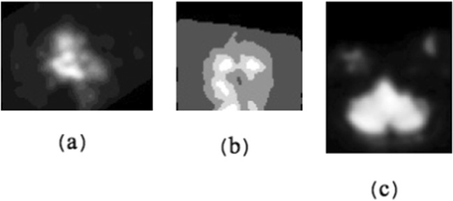
As we know, each 4D rs-fMRI data (three spatial dimensions + one temporal dimension) consists of several 3D sMRI data (three spatial dimensions). Each sMRI data belonged to a specific time point. We also know that each sMRI consists of several 2D spatial slices around x, y, and z coordinate axes (first spatial slice, …, middle spatial slice, ...., final spatial slice). By extracting the 2D first spatial slice of each sMRI belonged to a specific time point around x, y, and z axes, 4D rs-fMRI data were converted to three 3D images (two spatial dimensions + one temporal dimension). Figure 1a, b, and c are the 2D first spatial slice of each sMRI belonged to a specific time point across x, y, and z axes, respectively.
By applying fast Fourier transform on the time dimension of each 3D image and selecting the maximum frequency of each voxel, the dimensions of the images were reduced from three to two. This step produced images with 95 × 68, 79 × 68, and 79 × 95 dimensions, around the x, y, and z axes, respectively.
Fig. 1.
The 2D first spatial slice of each sMRI data belonged to a specific time point around three coordinate axes: (a) around x axis, (b) around y axis, and (c) around z axis
Convolutional Neural Networks
CNNs are one of the most important deep learning approaches in the tasks of classification and representation learning. In general, a CNN is a hierarchical neural network consists of three main layers: convolutional layers, pooling layers, and fully-connected layers [34]. There are two stages for training a CNN: a feed forward stage and a backward stage. In the feed forward stage, the prediction output is used to calculate the loss cost with the ground truth labels. In the backward stage, based on the calculated error, the gradient of each parameter is computed by the chain rules, and all the parameters are updated based on the gradients. After adequate iterations of these two stages, the learning of the CNN can be stopped [34].
Combining Multiple Networks
In order to achieve acceptable results, the results of several networks can be combined. In this paper, the results of multiple networks were fused using both dynamic (mixture of experts) and static (simple Bayes) combining classifiers methods, in order to classify autistic and non-autistic people based on rs-fMRI data around three coordinate axes (x, y, and z).
Mixture of CNN Experts
This section discusses the combined structure of mixture of CNN experts (MCNNEs), which is a new deep learning structure for achieving acceptable results in diagnosis of ASD. Firstly, the mixture of experts (MEs) method will be explained in the “Mixture of Experts” section.
Mixture of Experts
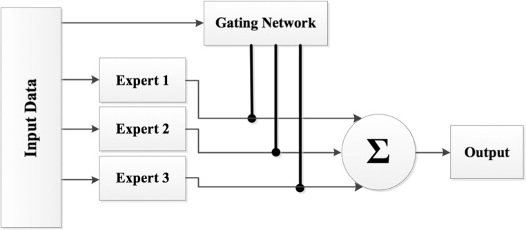
The MEs is one of the most popular dynamic models in combining classifiers. MEs was proposed by Jacobs et al. [35] based on the “divide and conquer” principle in which a gating network divide the problem space among a number of neural network experts. Figure 2 illustrates the structure of MEs with three experts and a gating network. In this paper, the CNN was used as experts and a gating network.
Fig. 2.
Structure of MEs with three experts and a gating network
MEs Learning Method
In MEs architecture, there is competitive learning process among experts; that is, the expert with fewer errors will be rewarded [35]. Let Ω = {ω1, ..., ωK}be the set of class labels, E = {E1, E2, ...,EL} the set of experts and x = {x1, x2, ...,xn} the input pattern vector. If the output of expert i for the input vector x is denoted as yi(x) and the final output of the architecture is denoted as Y(x), then we have:
| 1 |
| 2 |
where is the weight vector of expert i; the operator (.) is a symbol for dot product of two vectors of w and x; L is the number of experts and gi is the weight assigned to the output of expert i generated by the gating network. gi can be considered as an estimation of the probability function . In this architecture, the number of neurons in the output layer of the gating network is equal to the number of experts. The output of neuron i of the gating network can be defined by Eq. (3):
| 3 |
where is the connection weight between neuron t in the input layer to neuron i in the output layer of the gating network. Given the values of hi, the gi values are calculated from Eq. (4):
| 4 |
where gi is softmax function, so the sum of all the gi is equal to one. The biggest gi for an expert means that the expert is more capable of generating desired output.
For each expert i and gating network, the weights are updated according to the following rules:
| 5 |
| 6 |
where d(x) is ideal output vector for the input vector x, ηe, and ηg are learning rate for each expert i and gating network, respectively. Furthermore, ki can be defined by Eq. (7):
| 7 |
Structure of the Proposed MCNNEs
The general architecture of our proposed MCNNEs network is shown in Fig. 2. Experts and a gating network consist of three convolutional layers, three max pooling layers, and one fully connected layer. The architectural details of gating and expert networks are presented in Tables 2, 3, and 4, respectively. As can be observed, there are two differences among these architectures: the number of convolutional filters and the number of neurons in the fully connected layer. In this study, the non-linear activation function called rectified linear unit (ReLu) was used [36] in each convolutional layer. In addition, in order to prevent overfitting, dropout strategy with probability 0.5 was also employed [37] in the fully connected layer of each expert and gating network (Tables 2, 3, and 4). It should be noted that the binary softmax regression (logistic regression) was used as the classifier.
Table 2.
Architecture of expert 1 and gating network
| Input image | Layer | Layer type | Size | Output shape |
|---|---|---|---|---|
| Across x axis | 1 | Convolution + ReLu | Filters 8, kernel 3 × 3 | (8, 93, 66) |
| Across y axis | (8, 77, 66) | |||
| Across z axis | (8, 77, 93) | |||
| Across x axis | 2 | Max pooling | Kernel 2 × 2, stride 2 | (8, 46, 33) |
| Across y axis | (8, 38, 33) | |||
| Across z axis | (8, 38, 46) | |||
| Across x axis | 3 | Convolution + ReLu | filters: 8, kernel: 3 × 3 | (8, 44, 31) |
| Across y axis | (8, 36, 31) | |||
| Across z axis | (8, 36, 44) | |||
| Across x axis | 4 | Max pooling | Kernel 2 × 2, stride 2 | (8, 22, 15) |
| Across y axis | (8, 18, 15) | |||
| Across z axis | (8, 18, 22) | |||
| Across x axis | 5 | Convolution + ReLu | Filters 8, kernel 3 × 3 | (8, 20, 13) |
| Across y axis | (8, 16, 13) | |||
| Across z axis | (8, 16, 20) | |||
| Across x axis | 6 | Max pooling | kernel: 2 × 2, stride: 2 | (8, 10, 6) |
| Across y axis | (8, 8, 6) | |||
| Across z axis | (8, 8, 10) | |||
| Across x axis | 7 | Fully connected + ReLu dropout (rate 0.5) | 300 hidden units | 300 |
| Across y axis | 300 | |||
| Across z axis | 300 | |||
| Across x axis | 8 | Softmax | 2 | 2 |
| Across y axis | 2 | |||
| Across z axis | 2 |
Table 3.
Architecture of expert 2
| Input image | Layer | Layer type | Size | Output shape |
|---|---|---|---|---|
| Across x axis | 1 | Convolution + ReLu | Filters 10, Kernel: 3 × 3 | (10, 93, 66) |
| Across y axis | (10, 77, 66) | |||
| Across z axis | (10, 77, 93) | |||
| Across x axis | 2 | Max pooling | Kernel 2 × 2, stride 2 | (10, 46, 33) |
| Across y axis | (10, 38, 33) | |||
| Across z axis | (10, 38, 46) | |||
| Across x axis | 3 | Convolution + ReLu | Filters 10, kernel 3 × 3 | (10, 44, 31) |
| Across y axis | (10, 36, 31) | |||
| Across z axis | (10, 36, 44) | |||
| Across x axis | 4 | Max pooling | Kernel 2 × 2, stride 2 | (10, 22, 15) |
| Across y axis | (10, 18, 15) | |||
| Across z axis | (10, 18,22) | |||
| Across x axis | 5 | Convolution + ReLu | Filters 10, kernel 3 × 3 | (10, 20, 13) |
| Across y axis | (10, 16, 13) | |||
| Across z axis | (10, 16, 20) | |||
| Across x axis | 6 | Max pooling | Kernel 2 × 2, stride 2 | (10, 10, 6) |
| Across y axis | (10, 8, 6) | |||
| Across z axis | (10, 8, 10) | |||
| Across x axis | 7 | Fully connected + ReLu dropout (rate 0.5) | 400 hidden units | 400 |
| Across y axis | 400 | |||
| Across z axis | 400 | |||
| Across x axis | 8 | Softmax | 2 | 2 |
| Across y axis | 2 | |||
| Across z axis | 2 |
Table 4.
Architecture of expert 3
| Input Image | Layer | Layer type | Size | Output shape |
|---|---|---|---|---|
| Across x axis | 1 | Convolution + ReLu | Filters 12, kernel 3 × 3 | (12, 93, 66) |
| Across y axis | (12, 77, 66) | |||
| Across z axis | (12, 77, 93) | |||
| Across x axis | 2 | Max pooling | Kernel 2 × 2, stride 2 | (12, 46, 33) |
| Across y axis | (12, 38, 33) | |||
| Across z axis | (12, 38, 46) | |||
| Across x axis | 3 | Convolution + ReLu | Filters 12, kernel 3 × 3 | (12, 44, 31) |
| Across y axis | (12, 36, 31) | |||
| Across z axis | (12, 36, 44) | |||
| Across x axis | 4 | Max pooling | Kernel 2 × 2, stride 2 | (12, 22, 15) |
| Across y axis | (12, 18, 15) | |||
| Across z axis | (12, 18, 22) | |||
| Across x axis | 5 | Convolution + ReLu | Filters 12, kernel 3 × 3 | (12, 20, 13) |
| Across y axis | (12, 16, 13) | |||
| Across z axis | (12, 16, 20) | |||
| Across x axis | 6 | Max pooling | Kernel 2 × 2, stride 2 | (12, 10, 6) |
| Across y axis | (12, 8, 6) | |||
| Across z axis | (12, 8, 10) | |||
| Across x axis | 7 | Fully connected + ReLu dropout (rate 0.5) | 500 hidden units | 500 |
| Across y axis | 500 | |||
| Across z axis | 500 | |||
| Across x axis | 8 | Softmax | 2 | 2 |
| Across y axis | 2 | |||
| Across z axis | 2 |
Combining MCNNEs Using Simple Bayes Method
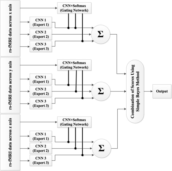
This section combines the MCNNEs networks with rs-fMRI input data around three coordinate axes (x, y, and z axes) using simple Bayes method in order to achieve acceptable results in the diagnosis of ASD and what was discussed in the “Dimension Reduction” section (Fig. 3). Firstly, this method will be explained in the “Simple Bayes method” section.
Fig. 3.
The combined MCNNEs
Simple Bayes Method
Static methods such as voting-based algorithms are based solely on the output label computed by each classifier. No expertise is considered. However, using Bayes theorem, the expertise of classifier is also considered. In this method, first, a confusion matrix, CMj, is formed according to the training data for each classifier Dj. Each row of the matrix represents the instances in an actual class while each column represents the instances in a predicted class. The elements of this matrix are denoted as cmj(k, s); that is, number of instances (input pattern x) belong to class ωk but classifier Dj is categorized into class ωs. cmj(s) can be calculated from Eq. (8).
| 8 |
Using the values of cmj(s) and cmj(k, s), the label matrix, LMj, can be calculated. This is a K × K matrix. The elements of this matrix are denoted as lmj(k, s) which are calculated by the following formula:
| 9 |
If S1, S2, …, SL are the labels that classifiers D1 to Dj assign to input pattern x, the estimation of the probability of actual label of input pattern x; ωi, is calculated from Eq. (10).
| 10 |
where is estimated based on the training data.
Transfer Learning
Transfer learning [38–42] is the process of using a pretrained CNN on dataset with a large number of samples, freezing the weights of the convolutional layers, replacing fully-connected layers and training these layers based on the small dataset. This method is very popular in CNN-based networks due to the fact that it accelerates the learning process and is one of the most effective strategies for training a CNN when the dataset may not be adequate to train a full structure of network.
Applying Transfer Learning in Diagnosis of ASD
The number of individuals ranging in age from 5 to 10 years in ABIDE I, ABIDE II, and the combination of them are 116, 343, and 459, respectively. In order to train CNNs, these are small datasets. Since CNNs are basically trained using a large-scale dataset, transfer learning strategy is one of the most effective strategies when having datasets with limited number of samples. Consequently, in this study, transfer learning strategy was applied as follows:
Formation of large datasets: Since each rs-fMRI data contains multiple sMRI images equal to the number of its time points, a large dataset considering the image of each time point as a sample was formed. As a result, the size of the created large ABIDE I, ABIDE II, and the combination of these two datasets is 19,808; 51,392; and 71,200; respectively.
Pretraining of the proposed CNNs: Large datasets generated in step 1 were used for pretraining of the proposed CNNs.
Using the pretrained CNNs from step 2, by freezing the weights of the initial layers and replacing the fully connected layer, only the fully connected and classifier layers of these networks were fine-tuned by these small datasets (datasets transformed to the frequency domain in the “Dimension reduction” section).
It should be noted that for transfer learning in medical imaging domain, natural image datasets or other medical imaging datasets can be used [43]. Furthermore, the transfer learning is possible between two different domains. In this study, transfer learning between two spatial and frequency domains was performed.
Implementation Details
In this research, the proposed model was implemented using Keras [44], one of the deep learning libraries written in Python. Keras can use both Theano [45, 46] and Tensorflow [47] as the backend. Keras with the Theano backend was used in this study. All the experiments were conducted using computer with an Intel Core i7 CPU (2.2 GHz) and 16 GB DDR3 memory. To train the model, the loss function and optimization methods are required. Since the problem is a binary classification, a binary cross-entropy loss function was used. In order to minimize loss function, adaptive moment estimation (Adam) and Adamax [48] optimization techniques were used. Adamax method was employed for pretraining of each expert and gating network. Furthermore, both Adam and Adamax approaches were used for fine-tuning of the last layers of proposed CNNs. A list of hyper-parameters used in this study is presented in Table 5.
Table 5.
Hyper-parameters
| Datasets | Batch size | Number of epochs | Regularization | Optimization method | Learning rate | Learning rate decay | Beta-1 | Beta-2 | Epsilon | |
|---|---|---|---|---|---|---|---|---|---|---|
| Pre-training | Fine-tuning | |||||||||
| ABIDE I | 30 | 22 | 50 | 0.01 | Adam | 0.01 | 0 | 0.9 | 0.999 | 1e-08 |
| Adamax | 0.002 | |||||||||
| ABIDE II | 20 | Adam | 0.01 | |||||||
| Adamax | 0.002 | |||||||||
| ABIDE I and ABIDE II | 20 | Adam | 0.01 | |||||||
| Adamax | 0.002 | |||||||||
Results
This section presents the results and analysis of proposed model, combination of pretrained MCNNEs using simple Bayes method. In order to do so, in the “Comparison of the Results of Combining MCNNEs with Each of These Networks on the Three Datasets” and the“Comparison of the Results of Combining MCNNEs with Combination of Simple CNNs on the Three Datasets” sections, we will compare the results of combination of three MCNNEs with the results of both each MCNNEs and combination of three simple CNNs. In each section, the results will be presented based on fine-tuning of the last layers of the CNNs in two stages. Adam and Adamax optimization methods were used in the first and second stages, respectively.
Comparison of the Results of Combining MCNNEs with Each of These Networks on the Three Datasets
Results Obtained from Adam Optimization Technique
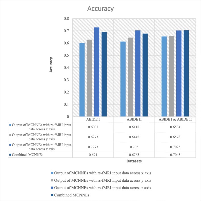
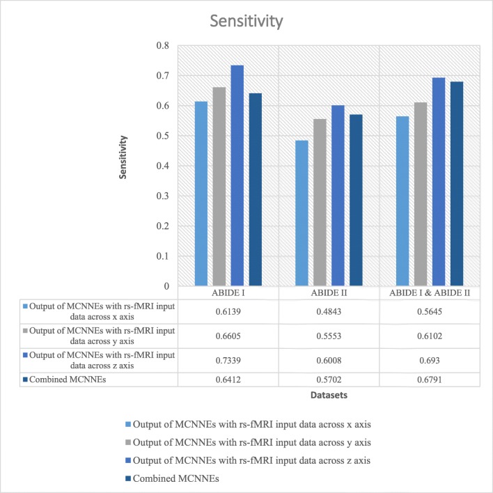
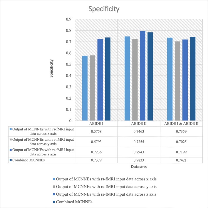
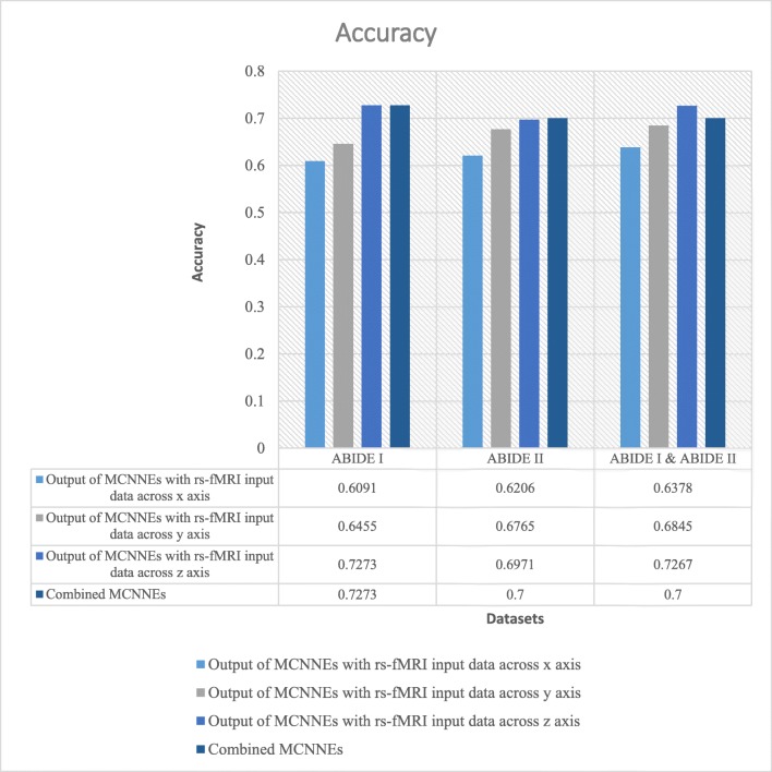
The classification accuracies, sensitivities, and specificities obtained from fine-tuning of the last layers of MCNNEs structures with rs-fMRI input data around three axes and combining these three structures using Adam optimization technique are shown in Figs. 4, 5, and 6 respectively.
Fig. 4.
Accuracies obtained from fine-tuning of the last layers of MCNNEs structures with rs-fMRI input data around three axes and combining them using Adam optimization technique
Fig. 5.
Sensitivities obtained from fine-tuning of the last layers of MCNNEs structures with rs-fMRI input data around three axes and combining them using Adam optimization technique
Fig. 6.
Specificities obtained from fine-tuning of the last layers of MCNNEs structures with rs-fMRI input data around three axes and combining them using Adam optimization technique
Referring to Fig. 4, it can be observed that in a combination of ABIDE I and ABIDE II datasets, the accuracy of combined MCNNEs using simple Bayes method is higher than accuracies obtained from singular MCNNEs with rs-fMRI input data around each axis. Meanwhile, in ABIDE I and ABIDE II datasets, in spite of obtaining less accuracy from the composition mode compared to maximum accuracy obtained from the single mode (around z axis), there was no significant difference. That is because, as it is shown in Table 6, by applying the t test to the accuracies obtained from tenfold cross validation, no significant difference was found between the maximum accuracy obtained from the singular structure (around z axis) and the accuracy of the combined MCNNEs (p (ABIDE I) = 0.6695, (p (ABIDE II) = 0.5658)).
Table 6.
Applying the t test to evaluation criteria obtained from tenfold cross validation on MCNNEs with maximum value obtained around one axis and combining MCNNEs according to rs-fMRI data based on first slices and using Adam and Adamax optimization techniques
| Optimization techniques | Datasets | p value | ||
|---|---|---|---|---|
| Accuracy | Sensitivity | Specificity | ||
| Adam | ABIDE I | 0.6695 | 0.3473 | – |
| ABIDE II | 0.5658 | 0.6519 | 0.7912 | |
| Combination of ABIDE I and ABIDE II | – | 0.8583 | – | |
| Adamax | ABIDE I | 1 | 0.7014 | 0.925 |
| ABIDE II | – | 0.8945 | – | |
| Combination of ABIDE I and ABIDE II | 0.2495 | 0.0906 | – | |
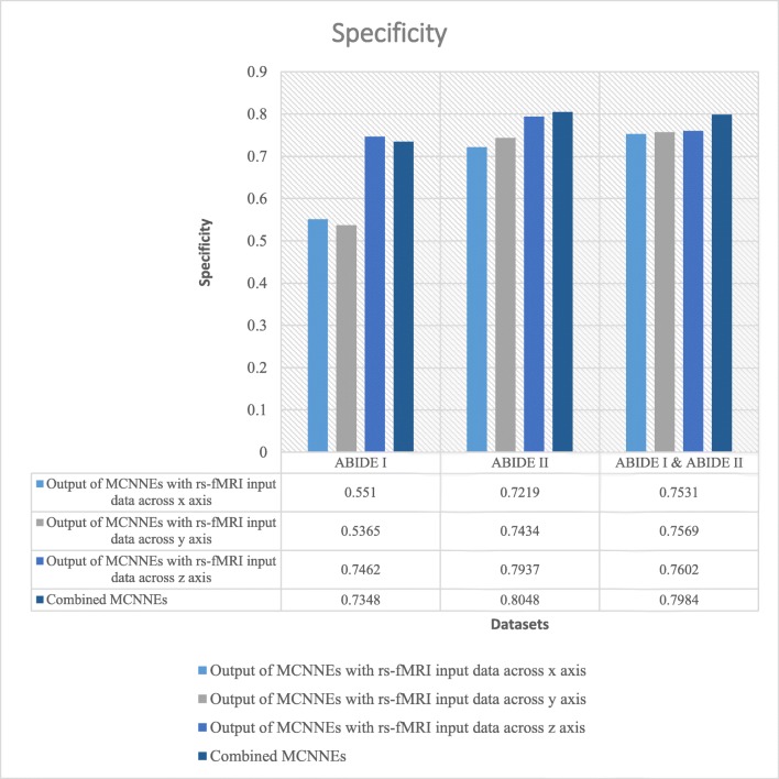
The results were also calculated in terms of other evaluation criteria such as sensitivity and specificity (Figs. 5 and 6). These figures also demonstrate that the composition mode will not provide better results compared to single networks. Furthermore, by applying the t test to the sensitivities and specificities which resulted from tenfold cross validation and calculating the p value, it can be concluded that there was no significant difference between maximum of these criteria obtained from each single network and their combination (Table 6).
Results Obtained from Adamax Optimization Technique
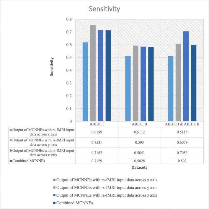
The classification results in terms of accuracies, sensitivities, and specificities obtained from fine-tuning of the last layers of MCNNEs structures with rs-fMRI input data around x, y, and z axes and combining them using Adamax optimization technique are shown in Figs. 7, 8, and 9, respectively.
Fig. 7.
Accuracies obtained from fine-tuning of the last layers of MCNNEs structures with rs-fMRI input data around three axes and combining them using Adamax optimization technique
Fig. 8.
Sensitivities obtained from fine-tuning of the last layers of MCNNEs structures with rs-fMRI input data around three axes and combining them using Adamax optimization technique
Fig. 9.
Specificities obtained from fine-tuning of the last layers of MCNNEs structures with rs-fMRI input data around three axes and combining them using Adamax optimization technique
As shown in Fig. 7, it can be observed that, unlike Adam optimization technique on ABIDE II dataset, the accuracy of combined MCNNEs using simple Bayes method is higher than accuracies obtained from each MCNNEs with rs-fMRI input data around each axis. Meanwhile, in ABIDE I dataset in composition mode, despite obtaining accuracy equal to maximum accuracy obtained around z axis, a sustainable result was obtained. That is because, as it is shown in Table 6, by applying the t test to the accuracies obtained from tenfold cross validation, there was no significant difference between the maximum accuracy and combined MCNNEs (p = 1). In the results obtained from a combination of these two datasets, the accuracy obtained from the composite mode is lower than the maximum accuracy (around z axis); however, by applying the t test (Table 6), a similar conclusion is drawn in terms of lack of a significant difference (p = 0.2495). Meanwhile, in Adam optimization technique, the accuracy obtained from the combined MCNNEs with simple Bayes method on a combination of these two datasets was higher compared to the each MCNNEs alone. Figures 8 and 9 represent other evaluation criteria such as sensitivity and specificity. As it was mentioned in the “Results Obtained from Adam Optimization Technique” section, t test was also applied to sensitivity and specificity of MCNNEs with maximum values and the result of combined MCNNEs. With consideration to the p value, it can be concluded that the null hypothesis of equality of the averages of these criteria cannot be rejected (Table 6).
Comparison of the Results of Combining MCNNEs with Combination of Simple CNNs on the Three Datasets
Results Obtained from Adam Optimization Technique
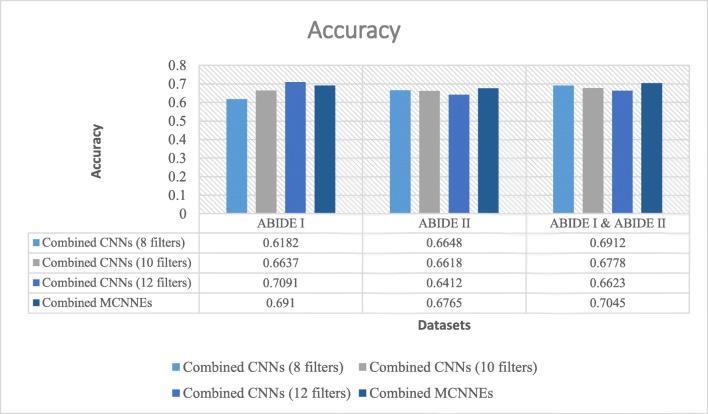
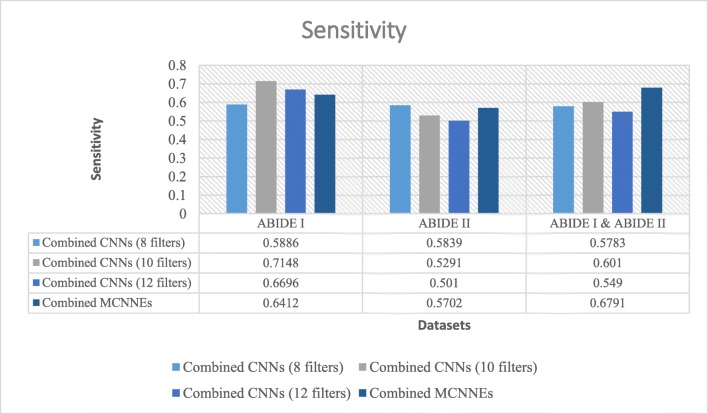
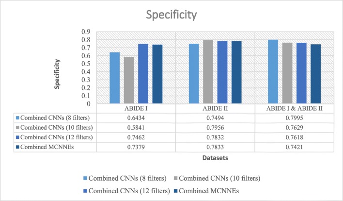
The performance measures namely, accuracy, sensitivity, and specificity obtained from fine-tuning of the last layers of combined MCNNEs and combined simple CNNs structures with rs-fMRI input data using Adam optimization technique are shown in Figs. 10, 11 and 12, respectively.
Fig. 10.
Accuracies obtained from fine-tuning of the last layers of combined MCNNEs and combined simple CNNs structures with 8, 10, and 12 filters with input data, using Adam optimization technique
Fig. 11.
Sensitivities obtained from fine-tuning of the last layers of combined MCNNEs and combined simple CNNs structures with 8, 10, and 12 filters with input data, using Adam optimization technique
Fig. 12.
Specificities obtained from fine-tuning of the last layers of combined MCNNEs and combined simple CNNs structures with 8, 10, and 12 filters with input data, using Adam optimization technique
Figure 10 illustrates that the best accuracy was obtained from combined MCNNEs on ABIDE II dataset and a combination of ABIDE I and ABIDE II datasets. The accuracy obtained from combined MCNNEs on ABIDE I dataset only fails to exceed the combined CNNs with 12 filters. In other words, by applying the t test, considering the p value, it can be concluded that there was no significant difference between the accuracy of combined MCNNEs and combined CNNs with 12 filters on ABIDE I dataset (p = 0.8384).
Figures 11 and 12 also represent sensitivity and specificity of combined MCNNEs and combined CNNs based on different filters. Figure 11 shows that only the sensitivity of combined MCNNEs exceeds combined CNNs in all structures with 8, 10 and 12 filters on a combination of two datasets. However, the sensitivity in the composite mode of MCNNEs on ABIDE I dataset is higher compared to combined CNNs with 8 filters. Also, on ABIDE II dataset, the sensitivity of combined MCCNEs is higher than combined CNNs with both 10 and 12 filters. In other words, despite obtaining less sensitivity from the composite mode of MCNNEs compared to combined CNNs, no significant difference was obtained (Table 7).
Table 7.
Applying the t test to evaluation criteria obtained from tenfold cross validation on combined CNNs with maximum value and combined MCNNEs according to rs-fMRI data based on first slices and using Adam and Adamax optimization techniques
| Optimization techniques | Datasets | p value | ||
|---|---|---|---|---|
| Accuracy | Sensitivity | Specificity | ||
| Adam | ABIDE I | 0.8384 | 0.4528 | 0.9438 |
| ABIDE II | – | 0.8541 | 0.7385 | |
| Combination of ABIDE I and ABIDE II | – | – | 0.3233 | |
| Adamax | ABIDE I | – | – | – |
| ABIDE II | – | 0.8784 | 0.78 | |
| Combination of ABIDE I and ABIDE II | 0.617 | 0.5967 | 0.3856 | |
Figure 12 shows that in terms of specificity, the composition mode of MCNNEs has obtained lower results compared to combined CNNs with 8, 10, and 12 filters on all three datasets whereas by applying the t test and considering the p values (p > 0.05) on all three datasets, the null hypothesis of equality of the averages of specifies cannot be rejected (Table 7).
Results Obtained from Adamax Optimization Technique
The classification accuracies, sensitivities, and specificities obtained from fine-tuning of the last layers of combined MCNNEs and combined simple CNNs structures with rs-fMRI input data using Adamax optimization technique are shown in Figs. 13, 14, and 15 respectively.
Fig. 13.
Accuracies obtained from fine-tuning of the last layers of combined MCNNEs and combined simple CNNs structures with 8, 10, and 12 filters with input data, using Adamax optimization technique
Fig. 14.
Sensitivities obtained from fine-tuning of the last layers of combined MCNNEs and combined simple CNNs structures with 8, 10, and 12 filters with input data, using Adamax optimization technique
Fig. 15.
Specificities obtained from fine-tuning of the last layers of combined MCNNEs and combined simple CNNs structures with 8, 10, and 12 filters with input data, using Adamax optimization technique
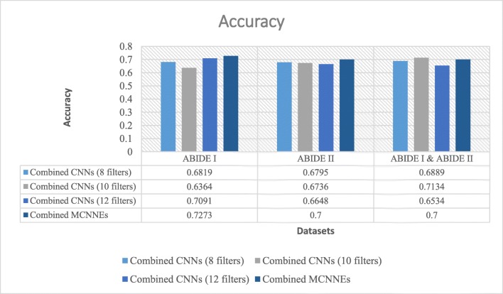
Figure 13 indicates that (unlike Adam optimization technique) on ABIDE I and ABIDE II datasets, the best accuracy was obtained from the combined MCNNEs. The accuracy obtained from combined MCNNEs on a combination of these two datasets (unlike Adam optimization technique) only fails to exceed the combined CNNs with 12 filters. In other words, by applying the t test, considering the p value, it can be concluded that there was no significant difference between the accuracy of combined MCNNEs and combined CNNs with 10 filters on a combination of ABIDE I and ABIDE II datasets (p = 0.617).
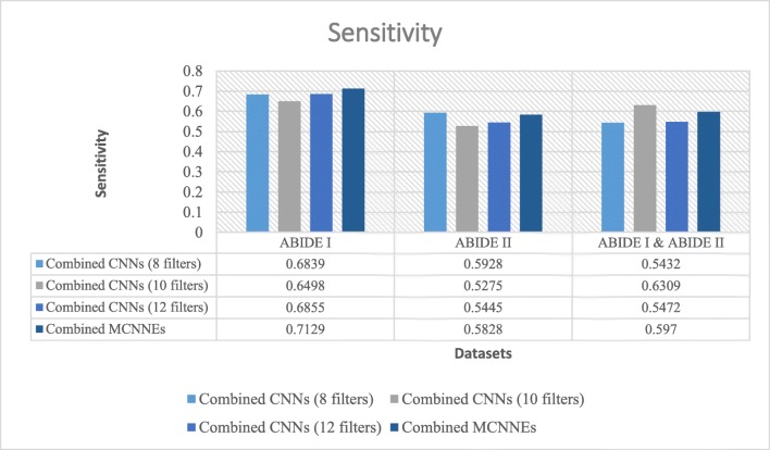
Moreover, Figs. 14 and 15 also represent criteria such as sensitivity and specificity of combined MCNNEs and combined CNNs based on different filters. Figure 14 demonstrates that only the sensitivity of combined MCNNEs exceeds combined CNNs in all structures with 8, 10, and 12 filters on ABIDE I dataset (unlike Adam optimization technique). However, the sensitivity in the composite mode of MCNNEs increased (unlike Adam optimization technique) on the combination of two ABIDE I and ABIDE II datasets compared to combined CNNs with 8 and 12 filters. Also, on ABIDE II dataset (similar to Adam optimization technique), the sensitivity of combined MCNNEs is higher compared to combined CNNs with 10 and 12 filters. In other words, despite obtaining less sensitivity in the composite mode of MCNNEs compared to combined CNNs, no significant difference was observed (Table 7).
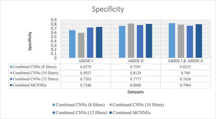
According to Fig. 15, unlike Adam optimization technique, the specificity of combined MCNNEs compared to combined CNNs is exceeded in all structures with 8, 10, and 12 filters only on ABIDE I dataset. Meanwhile, by applying the t test and considering the p values, according to Table 7, the null hypothesis of equality of the averages of specificities cannot be rejected.
Discussion
Accuracy, sensitivity, and specificity of our proposed method and previous works are summarized in Table 8. This research demonstrated the utility of combined MCNNEs model based on both Adam and Adamax optimization techniques and achieved higher accuracy, sensitivity, and specificity in comparison to models presented by Nielsen et al. [15], Ghiassian et al. [20], and Sen [21]. Previously, on ABIDE I dataset, the best accuracy, sensitivity, and specificity was 0.6502 [20], 0.62 [15], and 0.6475 [21], respectively. Our proposed model built with CNNs and Adamax optimization technique increased that accuracy (from 0.6502 to 0.7273), sensitivity (from 0.62 to 0.712), and specificity (from 0.6475 to 0.7348), respectively. It should be noted that the results obtained based on ABIDE II dataset and combination of ABIDE I and II datasets are not comparable to the results of the study of Nielsen et al. [15], Ghiassian et al. [20], and Sen [21], because no results have been published on them. However, acceptable classification results obtained on these datasets. CNN is able to extract hierarchical representations from large-scale data via multiple layers of nonlinear transformations. These transformations created representations that are beneficial for automated feature learning and classification task. With such discovering latent feature representation, particularly in case of complex fMRI datasets, it becomes easier to achieve better performance than traditional machine learning models that used hand-crafted features and considered only simple low-level features extracted from fMRI data. Furthermore, our combined MCNNEs architecture has its drawbacks as well. Deeper networks and especially presented model require more computational time and take longer time to train compared to the traditional methods such as support vector machine [20]. However, the computational burden of our proposed model was mostly related to the pretraining phase. In addition, despite increasing computational burden in combined networks compared to a single network, combined model exceeds a single model due to obtaining a more reliable, stable, and reproducible results. Another difficulty is the selection of appropriate parameters such as the number of convolutional filters and neurons in each fully connected layer and training hyper-parameters like learning rate, in order to obtain the best results and have acceptable computational burden. Furthermore, based on the experience gained in this research, the two following methods are recommended for future works and improvements of the results: Firstly, since the spatial dimensions of fMRI data are three, a 3D CNN can be designed instead of the 2D CNN presented in this study. Secondly, the CNNs proposed in this study were forward networks. Such networks are able to classify static images. Having sequences of images requires dynamic models. One solution for such problems is using recurrent neural network such as long short-term memory along with CNNs.
Table 8.
Comparison of results
| Datasets | Method | Accuracy | Sensitivity | Specificity | |
|---|---|---|---|---|---|
| ABIDE I | Nielsen et al. [15] | 0.6 | 0.62 | 0.58 | |
| Ghiassian et al. [20] | 0.6502 | – | – | ||
| Sen [21] | 0.6139 | 0.5781 | 0.6475 | ||
| Our proposed method | Adam | 0.691 | 0.641 | 0.737 | |
| Adamax | 0.7273 | 0.712 | 0.7348 | ||
| ABIDE II | Adam | 0.6765 | 0.570 | 0.783 | |
| Adamax | 0.7 | 0.582 | 0.804 | ||
| Combination of ABIDE I and ABIDE II | Adam | 0.7045 | 0.679 | 0.7421 | |
| Adamax | 0.7 | 0.59 | 0.798 | ||
Conclusions
This study presented an intelligent image-based computer-aided detection system for diagnosis of ASD based on rs-fMRI data of subjects ranging in age from 5 to 10 years from the ABIDE I and ABIDE II datasets. This system is based on CNNs using “combining classifiers,” both dynamic (mixture of experts) and static (simple Bayes) approaches, and “transfer learning” strategy. Some of the benefits of this model include achieving acceptable results and overcoming the challenge of obtaining dataset with sufficient samples in medical imaging domain. In addition, compared to the previous methods, researchers and specialists will be able to automatically extract features and classify images in a unique structure. In this paper, the results of diagnosis of ASD increased compared to the results of previous studies based on ABIDE I dataset. Moreover, acceptable classification results were obtained on the ABIDE II and the combination of ABIDE I and ABIDE II datasets. Furthermore, Adam and Adamax optimization techniques were employed. According to the obtained results on all three datasets, ABIDE I, ABIDE II, and the combination of them, it was observed that Adamax optimizer effectively tends to have smaller errors compared to Adam optimizer. We can conclude that the proposed architecture can be considered as an efficient tool for diagnosis of ASD in young children. From another perspective, this proposed method can be applied to analyzing fMRI data related to brain dysfunctions.
Acknowledgments
We thank the Autism Brain Imaging Data Exchange (ABIDE) for generously sharing their data with scientific community.
Compliance with Ethical Standards
Conflict of Interest
The authors declare that they have no conflict of interest.
Footnotes
Publisher’s Note
Springer Nature remains neutral with regard to jurisdictional claims in published maps and institutional affiliations.
Contributor Information
Maryam Akhavan Aghdam, Email: maryam_akhavan_aghdam@yahoo.com.
Arash Sharifi, Email: a.sharifi@srbiau.ac.ir.
Mir Mohsen Pedram, Email: pedram@khu.ac.ir.
References
- 1.Crosson B, Ford A, McGregor KM, Meinzer M, Cheshkov S, Li X, Walker-Baston D, Briggs RW. Functional imaging and related techniques: An introduction for rehabilitation researchers. J Rehabil Res Dev. 2010;47(2):vii–xxxiv. doi: 10.1682/JRRD.2010.02.0017. [DOI] [PMC free article] [PubMed] [Google Scholar]
- 2.Sarraf S, Sun J: Functional Brain Imaging: A Comprehensive Survey. arXiv preprint arXiv:1602.02225, 2005.
- 3.Fox MD, Snyder AZ, Vincent JL, Corbetta M, Essen DCV, Raichle ME. The human brain is intrinsically organized into dynamic, anticorrelated functional networks. Proc Natl Acad Sci USA. 2005;102(27):9673–9678. doi: 10.1073/pnas.0504136102. [DOI] [PMC free article] [PubMed] [Google Scholar]
- 4.Buckner RL, Andrews-Hanna JR, Schacter DL. The brain’s default network. Ann NY Acad Sci. 2008;1124:1–38. doi: 10.1196/annals.1440.011. [DOI] [PubMed] [Google Scholar]
- 5.Wang J, Zuo X, He Y: Graph-based network analysis of resting-state functional MRI. Front Syst Neurosci, 2010. 10.3389/fnsys.2010.00016 [DOI] [PMC free article] [PubMed]
- 6.Suk HI, Wee CY, Lee SW, Shen D. State-space model with deep learning for functional dynamics estimation in resting-state fMRI. Neuroimage. 2016;129:292–307. doi: 10.1016/j.neuroimage.2016.01.005. [DOI] [PMC free article] [PubMed] [Google Scholar]
- 7.Levy SE, Mandell DS, Schultz RT. Autism. Lancet. 2009;374(9701):1627–1638. doi: 10.1016/S0140-6736(09)61376-3. [DOI] [PMC free article] [PubMed] [Google Scholar]
- 8.Coleman M, Gillberg C. The Autisms. Oxford: Oxford University Press; 2012. [Google Scholar]
- 9.Waterhouse L. Rethinking Autism: Variation and Complexity. London: Academic Press; 2013. [Google Scholar]
- 10.Fernell E, Eriksson MA, Gillberg C. Early diagnosis of autism and impact on prognosis: a narrative review. Clin Epidemiol. 2013;5:33–43. doi: 10.2147/CLEP.S41714. [DOI] [PMC free article] [PubMed] [Google Scholar]
- 11.Pennington Malinda L., Cullinan Douglas, Southern Louise B. Defining Autism: Variability in State Education Agency Definitions of and Evaluations for Autism Spectrum Disorders. Autism Research and Treatment. 2014;2014:1–8. doi: 10.1155/2014/327271. [DOI] [PMC free article] [PubMed] [Google Scholar]
- 12.Yerys BE, Pennington BF. How do we establish a biological marker for a behaviorally defined disorder? Autism as a test case. Autism Res. 2011;4(4):239–241. doi: 10.1002/aur.204. [DOI] [PubMed] [Google Scholar]
- 13.Plitt M, Barnes KA, Martin A. Functional connectivity classification of autism identifies highly predictive brain features but falls short of biomarker standards. Neuroimage Clin. 2014;7:359–366. doi: 10.1016/j.nicl.2014.12.013. [DOI] [PMC free article] [PubMed] [Google Scholar]
- 14.Di Martino A, Yan CG, Li Q, Denio E, Castellanos FX, Alaerts K, Anderson JS, Assaf M, Bookheimer SY, Dapretto M, Deen B, Delmonte S, Dinstein I, Ertl-Wagner B, Fair DA, Gallagher L, Kennedy DP, Keown CL, Keysers C, Lainhart JE, Lord C, Luna B, Menon V, Minshew NJ, Monk CS, Mueller S, Müller RA, Nebel MB, Nigg JT, O’Hearn K, Pelphrey KA, Peltier SJ, Rudie JD, Sunaert S, Thioux M, Tyszka JM, Uddin LQ, Verhoeven JS, Wenderoth N, Wiggins JL, Mostofsky SH, Milham MP. The autism brain imaging data exchange: towards a large-scale evaluation of the intrinsic brain architecture in autism. Mol Psychiatry. 2014;19(6):659–667. doi: 10.1038/mp.2013.78. [DOI] [PMC free article] [PubMed] [Google Scholar]
- 15.Nielsen JA, Zielinski BA, Fletcher PT, Alexander AL, Lange N, Bigler ED, Lainhart JE, Anderson JS: Multisite functional connectivity MRI classification of autism: ABIDE results. Front. Hum. Neurosci 7(599), 2013. 10.3389/fnhum.2013.00599 [DOI] [PMC free article] [PubMed]
- 16.Anderson JS, Nielsen JA, Froehlich AL, DuBray MB, Druzgal TJ, Cariello AN, Cooperrider JR, Zielinski BA, Ravichandran C, Fletcher PT, Alexander AL, Bigler ED, Lange N, Lainhart JE. Functional connectivity magnetic resonance imaging classification of autism. Brain. 2011;134(12):3742–3754. doi: 10.1093/brain/awr263. [DOI] [PMC free article] [PubMed] [Google Scholar]
- 17.Uddin LQ, Supekar K, Lynch CJ, Khouzam A, Phillips J, Feinstein C, Ryali S, Menon V. Salience network-based classification and prediction of symptom severity in children with autism. JAMA Psychiatry. 2013;70(8):869–879. doi: 10.1001/jamapsychiatry.2013.104. [DOI] [PMC free article] [PubMed] [Google Scholar]
- 18.Bell AJ, Sejnowski TJ. An information-maximization approach to blind separation and blind deconvolution. Neural Comput. 1995;7(6):1129–1159. doi: 10.1162/neco.1995.7.6.1129. [DOI] [PubMed] [Google Scholar]
- 19.McKeown MJ, Makeig S, Brown GG, Jung TP, Kindermann SS, Bell AJ, Sejnowski TJ. Analysis of fMRI data by blind separation into independent spatial components. Hum Brain Mapp. 1998;6(3):160–188. doi: 10.1002/(SICI)1097-0193(1998)6:3<160::AID-HBM5>3.0.CO;2-1. [DOI] [PMC free article] [PubMed] [Google Scholar]
- 20.Ghiassian S, Greiner R, Jin P, Brown MRG. Using functional or structural magnetic resonance images and personal characteristic data to diagnose ADHD and autism. PLos ONE. 2016;11(12):e0166934. doi: 10.1371/journal.pone.0166934. [DOI] [PMC free article] [PubMed] [Google Scholar]
- 21.Sen B: Generalized Prediction Model for Detection of Psychiatric Disorders. Master Thesis, University of Alberta, 2016.
- 22.Plis SM, Hjelm D, Salakhutdinov R, Allen EA, Bockholt HJ, Long JD, Johnson HJ, Paulsen J, Turner JA, Calhoun VD: Deep learning for neuroimaging: a validation study. Front Neurosci 8, 2014. 10.3389/fnins.2014.00229 [DOI] [PMC free article] [PubMed]
- 23.Olshausen BA. Emergence of simple-cell receptive field properties by learning a sparse code for natural images. Nature. 1996;381(6583):607–609. doi: 10.1038/381607a0. [DOI] [PubMed] [Google Scholar]
- 24.Suk HI, Lee SW, Shen D. Hierarchical feature representation and multimodal fusion with deep learning for AD/MCI diagnosis. Neuroimage. 2014;101:569–582. doi: 10.1016/j.neuroimage.2014.06.077. [DOI] [PMC free article] [PubMed] [Google Scholar]
- 25.Suk HI, Lee SW, Shen D. Latent feature representation with stacked auto-encoder for AD/MCI diagnosis. Brain Struct Funct. 2015;220(2):841–859. doi: 10.1007/s00429-013-0687-3. [DOI] [PMC free article] [PubMed] [Google Scholar]
- 26.Sarraf S, Tofighi G: Classification of Alzheimer’s Disease Using fMRI Data and Deep Learning Convolutional Neural Networks. arXiv preprint arXiv:1603.08631, 2016.
- 27.Available at: http://image-net.org/challenges/LSVRC/
- 28.Russakovsky O, Deng J, Su H, Krause J, Satheesh S, Ma S, Huang Z, Karpathy A, Khosla A, Bernstein M, Berg AC, Fei-Fei L. Imagenet large scale visual recognition challenge. Int J Comput Vis. 2015;115(3):211–252. doi: 10.1007/s11263-015-0816-y. [DOI] [Google Scholar]
- 29.Available at: http://fcon_1000.projects.nitrc.org/indi/abide/
- 30.Jenkinson M, Smith SM: Pre-Processing of BOLD FMRI Data. Oxford University Centre for Functional MRI of the Brain (FMRIB), 2006.
- 31.Available at: http://www.fil.ion.ucl.ac.uk/spm/software/spm8/
- 32.Bowman FD, Guo Y, Derado G. Statistical approaches to functional neuroimaging data. Neuroimaging Clin N Am. 2007;17(4):441–458. doi: 10.1016/j.nic.2007.09.002. [DOI] [PMC free article] [PubMed] [Google Scholar]
- 33.Hermans E: SPM8 Starters Guide, 2011. http://www.ernohermans.com.
- 34.Guo Y, Liu Y, Oerlemans A, Lao S, Wu S, Lew MS. Deep learning for visual understanding: a review. Neurocomputing. 2016;187:27–48. doi: 10.1016/j.neucom.2015.09.116. [DOI] [Google Scholar]
- 35.Jacobs RA, Jordan MI, Steven JN, Georey EH. Adaptive mixtures of local experts. Neural Computation. 1991;3(1):79–87. doi: 10.1162/neco.1991.3.1.79. [DOI] [PubMed] [Google Scholar]
- 36.Nair V, Hinton GE: Rectified linear units improve restricted Boltzmann machines. In Proceedings of the International Conference on Machine Learning (ICML), 2010.
- 37.Hinton GE, Srivastava N, Krizhevsky A, Sutskever I, Salakhutdinov RR: Improving Neural Networks by Preventing Co-adaptation of Feature Detectors. arXiv preprint arXiv: 1207.0580, 2012.
- 38.Ciresan DC, Meier U, Schmidhuber J: Transfer learning for Latin and Chinese characters with deep neural networks. In: Proceedings of the IEEE International Joint Conference on Neural Networks (IJCNN), 2012.
- 39.Ren JSJ, Xu L: On vectorization of deep convolutional neural networks for vision tasks. In: Proceedings of the Association for the Advancement of artificial intelligence (AAAI), the 29th international conference on artificial intelligence, 2015.
- 40.Ackey S, Kundegorski ME, Devereux M, Breckon TP: Transfer learning using convolutional neural networks for object classification within X-ray baggage security imagery. In: Proceedings of the IEEE International Conference on Image Processing (ICIP), pp 1057–1061, 2016. 10.1109/ICIP.2016.7532519
- 41.Singh D, Garzon P: Using Convolutional Neural Networks and Transfer Learning to Perform Yelp Restaurant Photo Classification, 2016.
- 42.Tan C, Sun F, Kong T, Zhang W, Yang C, Liu C: A Survey on Deep Transfer Learning, arXiv preprint arXiv: 1808.01974, 2018.
- 43.Shin HC, Roth HR, Gao M, Lu L, Xu Z, Nogues I, Yao J, Mollura D, Summers RM. Deep convolutional neural networks for computer-aided detection: CNN architectures, dataset characteristics and transfer learning. IEEE Trans Med Imaging. 2016;35(5):1285–1298. doi: 10.1109/TMI.2016.2528162. [DOI] [PMC free article] [PubMed] [Google Scholar]
- 44.Chollet F: Keras: Deep Learning Library for Theano and TensorFlow. 2015. https://github.com/fchollet/keras
- 45.Bastien F, Lamblin P, Pascanu R, Bergstra J, Goodfellow IJ, Bergeron A, Bouchard N, Warde-Farley D, Bengio Y: Theano: New features and speed improvements. In: Proceedings of the workshop on deep learning and unsupervised feature learning Neural Information Processing Systems (NIPS), 2012.
- 46.Theano Development Team: Theano: A Python framework for fast computation of mathematical expressions. arXiv preprint arXiv:1605.02688.
- 47.Abadi M, Barham P, Chen J, Chen Z, Davis A, Dean J, Devin M, Ghemawat S, Irving G, Isard M, Kudlur M, Levenberg J, Monga R, Moore S, Murray DG, Steiner B, Tucker P, Vasudevan V, Warden P, Wicke M, Yu Y, Zheng X: Tensorflow: A system for large-scale machine learning. arXiv preprint arXiv:1605.08695, 2016.
- 48.Kingma DP, Ba JL: Adam: A method for stochastic optimization. In: Proceedings of the international conference on learning representations (ICLR), 2015.


