A Linear Regression Predictor for Identifying N⁶-Methyladenosine Sites Using Frequent Gapped K-mer Pattern

Abstract

N6-methyladenosine (m⁶A) is one of the most common and abundant modifications in RNA, which is related to many biological processes in humans. Abnormal RNA modifications are often associated with a series of diseases, including tumors, neurogenic diseases, and embryonic retardation. Therefore, identifying m⁶A sites is of paramount importance in the post-genomic age. Although many lab-based methods have been proposed to annotate m⁶A sites, they are time consuming and cost ineffective. In view of the drawbacks of the intrinsic methods in RNA sequence recognition, computational methods are suggested as a supplement to identify m⁶A sites. In this study, we develop a novel feature extraction algorithm based on the frequent gapped k-mer pattern (FGKP) and apply the linear regression to construct the prediction model. The new predictor is used to identify m⁶A sites in the Saccharomyces cerevisiae database. It has been shown by the 10-fold cross-validation that the performance is better than that of recent methods. Comparative results indicate that our model has great potential to become a useful and effective tool for genome analysis and gain more insights for locating m⁶A sites.

Introduction

Over 100 modifications occur in RNA.¹ The functions of internal modifications of mRNA are used to keep the stability of mRNA, and the most common internal modifications of mRNA include N⁶-methyladenosine (m⁶A), N¹-methyladenosine (m¹A), 5-methylcytosine (m⁵C). Among them, global scientists have verified many enzymes that m⁶A engages, such as histone demethylases, methylase, and methylation recognition enzyme.² Abnormal m⁶A modifications are often related to a series of diseases, including tumors, neurogenic diseases, and embryonic retardation.³ RNA m⁶A was first observed in 1970s.⁴ Since then, m⁶A is found in a wide spectrum of all living organisms and linked to many important roles of biological activities, including mRNA splicing, stability, nuclear processing, and immune response.5, 6, 7, 8 Therefore transcriptome-wide annotation of m⁶A sites will be helpful to understand its biological functions.

In the past few years, high-throughput sequencing techniques such as MeRIPSeq⁹ and m⁶A-seq¹⁰ have identified m⁶A peaks in Saccharomyces cerevisiae, Mus musculus, and Homo sapiens. At the same time, the miCLIP technique¹¹ was proposed to provide the recognition method of m⁶A sites in the human transcriptome. However, in consideration of the biological inherent reliance of the techniques,¹² they are still neither budget nor time efficient in performing transcriptome-wide analysis.

Although lab-based technologies have been widely applied to identify m⁶A, some cost-effective computational methods are developed in assisting the process as well. To identify methylated m⁶A sites, building a high-resolution database is of paramount importance in predicting m⁶A sites. Using the high-resolution database of Saccharomyces cerevisiae constructed by Schwartz et al.,¹³ Chen et al.14, 15, 16, 17, 18 proposed a series of predictors such as “iRNA-Methyl,” “M6ATH,” “MethyRNA,” “iRNA-3typeA” and “iRNA(m6A)-PseDNC,” which formulated RNA sequences by using different combinations of feature extractions and classifiers to make predictions. Feng et al.¹⁹ used a method called “iRNA-PseColl,” which incorporated collective features of the RNA sequence elements into PseKNC to make predictions. Jaffrey et al.¹¹ built a single-nucleotide resolution map of m⁶A sites across Homo sapiens. More recently, Chen et al.²⁰ proposed a support-vector-machine-based method to predict m⁶A sites in Arabidopsis thaliana. As mentioned in some references, well-established ensemble classifiers have been proven to outperform single classifiers.21, 22, 23 Based on this, Wei et al.²⁴ thus proposed an m⁶A predictor by constructing an ensemble classifier based on the support vector machine (SVM) to successfully improve the predictive performance. Wei et al.^25,26 have also done a lot of research with the ensemble classifier, which has great significance for reference in our study.

In this article, we propose a novel method for the identification of m⁶A sites within RNA sequences. As for feature representation, we use the frequent gapped k-mer pattern (FGKP) discovery algorithm to mainly capture the properties in RNA sequences. In the predictive model, we use the linear regression to discriminate the positive and negative samples. Experimental results show that our model outperformed other existing methods in the literature under the 10-fold cross-validation test.

Results

Several diseases have their underlying causes in RNA,^27,28 including cancers.29, 30, 31 In our study, we combined the advantage of effective extraction of frequent gapped k-mer (FGK) and the strong ability of classification of the linear predictive model to create a powerful predictive tool in order to discriminate the positive and negative samples of m⁶A. The learning machine that we used was logistic regression (LR). We have experimented with our predictor in the Saccharomyces cerevisiae genome using 10-fold cross-validation. It turns out that our model is superior to M6A-HPCS, the recent classifier in this area, and also has a better performance than other feature extractions and different parameters within our model. We anticipate that it will shed some light on genome analysis in future practice.

Four Evaluation Metrics

In general, the following four metrics are used to measure the quality of a predictor:³² sensitivity (SN), specificity (SP), accuracy (ACC), and Matthews correlation coefficient (MCC). These metrics were first introduced by Chou³³ and then they were widely applied to a wide range of biological areas (see Liu et al.,34, 35, 36, 37 Ehsan et al.,³⁸ Feng et al.,¹⁹ Song et al.,³⁹ Lin et al.,⁴⁰ and Xu et al.^40,41). Their definitions are as follows:

$$\mathit{SP}=\frac{\mathit{TN}}{\mathit{TN}+\mathit{FP}}\times 100\%$$ (Equation 1)

$$\mathit{SN}=\frac{\mathit{TP}}{\mathit{TP}+\mathit{FN}}\times 100\%$$ (Equation 2)

$$\mathit{ACC}=\frac{\mathit{TP}+\mathit{TN}}{\mathit{TP}+\mathit{FN}+\mathit{TN}+\mathit{FP}}\times 100\%$$ (Equation 3)

and

$$\mathit{MCC}=\frac{\mathit{TP}\times \mathit{TN}-\mathit{FP}\times \mathit{FN}}{\sqrt{\left(\mathit{TP}+\mathit{FN}\right)\left(\mathit{TN}+\mathit{FP}\right)\left(\mathit{TP}+\mathit{FP}\right)\left(\mathit{TN}+\mathit{FN}\right)}}$$ (Equation 4)

where TP, TN, FP, and FN are true positive, true negative, false positive, and false negative, respectively. In this research, TP represents the true m⁶A site predicted correctly, TN represents the non-m⁶A site predicted incorrectly, FP represents the non-m⁶A site predicted incorrectly as the true m⁶A site, and FN represents the non-m⁶A site predicted correctly as the non-m⁶A site. The values of SN, SP, ACC, are between 0 and 1. The closer to 1 they get, the more accuracy our model achieves; the value of MCC is between −1 and 1. The larger the value that MCC gets, the better performance our prediction model obtains.

Cross-Validation

Normally, three types of validation are used to derive the metric values: independent test sets, subsampling (or K-fold cross-validation), and the jackknife test (or LOOCV). Although the jackknife test can fully train the data we already have to acquire a more accurate classifier, and it has definite sampling and error estimation based on the specific dataset, the jackknife test is not a time-efficient method compared with the other two types of validation. In this article, we adopted the 10-fold cross-validation method used by many researchers42, 43, 44 in this area.

ROC Curve

ROC curve (also called the sensitivity curve) is the abbreviation for receiver operating characteristic curve. Every point on the curve reflects the same sensitivity. They react to the same signal simulation in the different judgment standards. Therefore, the ROC curve can be generally treated as the overall performance in the binary classification problems. The ROC curve is normally plotted with the x-axis true-positive rate (TPR) and the y-axis false-positive rate (FPR) in the different thresholds of the classification. We can understand the TPR as the sensitivity as described earlier, and the FPR can be computed as 1 − specificity. The area under the ROC curve (AUROC) can also be calculated. The AUROC is the indicator of the performance of a predictor. The AUROC ranges from 0.5 to 1. The closer the AUROC score of a predictor to 1, the better and more robust the predictor we can reckon, and we can deem the AUROC score of 0.5 of a predictor as a random predictor.

Discussion

Comparison among Different Feature Extractions

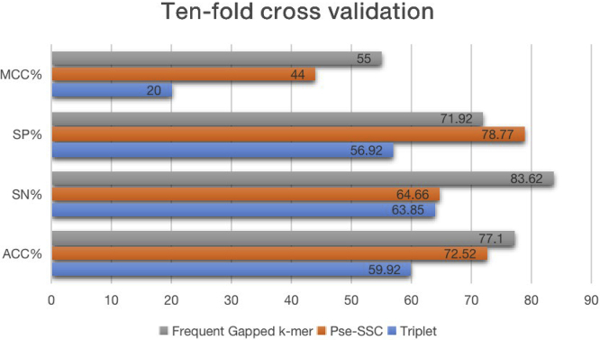
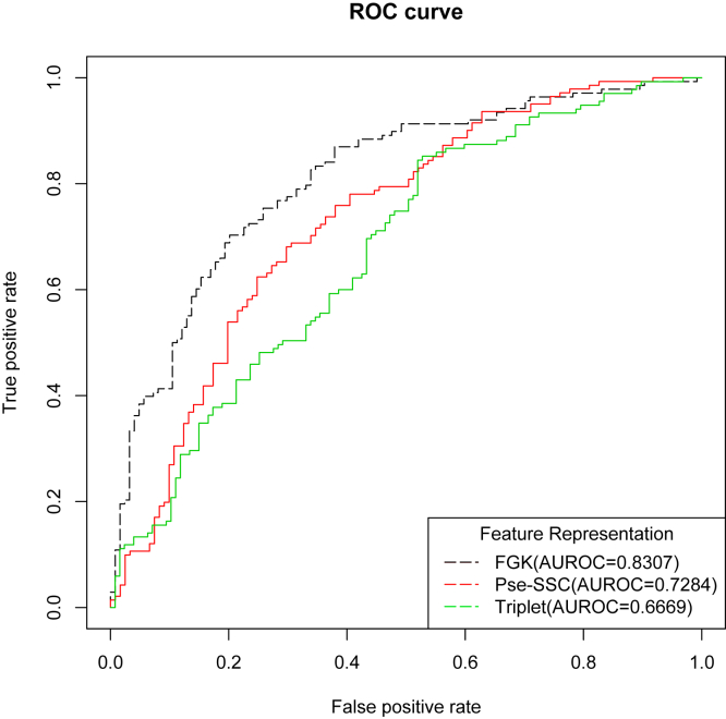
To justify our feature extraction technique, we make comparisons with two of the most commonly used feature representation techniques, Triplet and Pse-SSC, and this shows that the FGK method gets the much better performance than the other two feature representations. We show the result in Table 1, and from Figure 1, we can see the graphical comparisons from four different evaluation metrics. The FGK leads Pse-SSC by 4% and Triplet by 17% for the ACC, and for the MCC metric, FGK outnumbers its counterparts by over 10%. From Figure 2, we can see the effects of three different feature extractions from their ROC curves. The larger areas under the curve we get, the better performance the method achieves. Also, we can also see from Table 1 that our feature representation is 63.2% and 16.4% higher than features Pse-SSC and Triplet, respectively.

Table 1.

Comparison of Different Feature Extractions

Feature	SP (%)	SN (%)	ACC (%)	MCC	AUROC
Triplet	56.92	63.85	59.92	0.20	0.6669
Pse-SSC	78.77	64.66	72.52	0.44	0.7284
Frequent gapped k-mer	71.92	83.62	77.10	0.55	0.8307

Figure 1.

Performance of Different Feature Extractions Using 10-Fold Cross-validation

Here, we compare the effect of our feature extraction (FGK) with Pse-SSC and Triplet methods.

Figure 2.

ROC Curves of Frequent Gapped K-mer, Pse-SSC, and Triplet and Their AUROC Values

Comparison with Other Classifiers

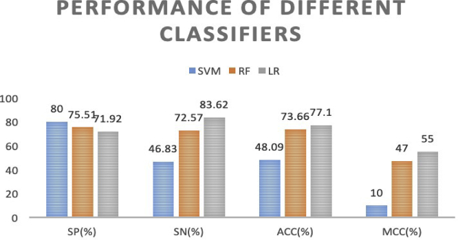
In Table 2, we compare LR with SVM and random forest (RF). The reason for choosing SVM and RF for comparison is because SVM^20,21,45,46 and RF^5,47, 48, 49, 50 are two of the most widely used classifiers in bioinformatics. Although the SP of the proposed method is lower than those of SVM and RF, its SN, ACC, and MCC are higher than those of SVM and RF, indicating that the performance of the LR-based model can effectively discriminate the m⁶A sites in Saccharomyces cerevisiae. We can see the overall performance of three classifiers in Figure 3. In this figure, we can see that, although the SP of LR performs poorly compared to that of the other two classifiers, the other three metrics are much better than the rest for the two predictors. The ACC of LR is far better than that of SVM, topping by almost 30% and slightly exceeding by 3.5% the ACC of RF.

Table 2.

Performance Comparison of Different Classifiers

Classifier	SP (%)	SN (%)	ACC (%)	MCC
SVM	80	46.83	48.09	0.10
RF	75.51	72.56	73.66	0.47
LR	71.92	83.62	77.10	0.55

Figure 3.

Comparison of Performances among the LR Classifier and Other Popular Classifiers (SVM and RF) with the Same Learning Feature Representations on the S. cerevisiae Dataset

Comparison with Different Parameters

In Table 3, we compared the model prediction performance of linear regression using different parameters and found that, with parameters k = 4 and γ = 0.025, we get the most desirable result. The classifier with parameters k = 5 and γ = 0.05 is almost 25% higher than its counterpart in ACC.

Table 3.

Performance Comparison of Different Parameters in Our Model

Classifier	SP (%)	SN (%)	ACC (%)	MCC
LR (k = 5, γ = 0.05)	73.53	73.81	73.66	0.47
LR( k = 4, γ = 0.025)	71.92	83.62	77.10	0.55

Comparison with Existing Predictors

To evaluate the performance of our proposed predictor, we compared our predictor with two existing predictors, iRNA-Methyl¹⁴ and M6A-HPCS.⁵¹ The reason to choose these two predictors for comparison is that they have been reported to achieve outstanding performance in m⁶A site identification. For fairness of comparison, all compared predictors are trained and validated on the same benchmark dataset. The results are summarized in Table 4. It can be observed that, among the compared predictors, the proposed model obtains the best performance in terms of ACC and MCC, with 77.10% and 55%, respectively. Compared with the best of the existing predictors, M6A-HPCS, our classifier performance is about 10% higher for ACC and 20% higher for MCC.

Table 4.

Comparison of M6APred-FG with Other Well-Known Classifiers

Prediction Method	SP (%)	SN (%)	ACC (%)	MCC
iRNA-Methyl	60.63	70.59	65.59	0.29
M6A-HPCS	62.89	71.77	67.33	0.35
iRNA-Freq	71.92	83.62	77.10	0.55

Materials and Methods

Framework of the Proposed Predictor

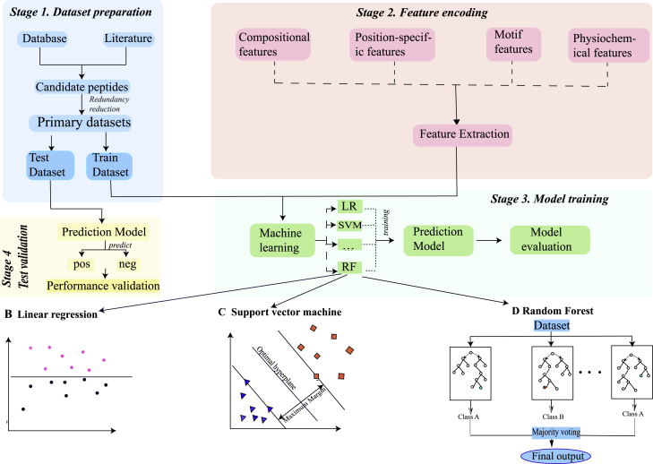
Figure 4 shows the flowchart of the proposed predictor. The first stage is to collect data from verified databases and relevant literature.^14,15,52 In this research, we use the organized dataset from Chen et al.’s¹⁴ work. The second stage is feature encoding. This stage includes feature representation and feature optimization. Feature representation means extracting characteristics of RNA sequences using various feature descriptors, including composition features like Dinucleotide-based auto covariance (DAC), physicochemical features like PC-PseDNC-General, and our newly found FGKP. The final stage is to train the machine learning model (i.e., SVM, RF, and linear regression) using the feature extraction from the last stage. The predictive model constructed is based on the feature extraction mentioned earlier and validated through validation methods. In this study, we used the 10-fold cross-validation test.

Figure 4.

Flowchart of the Proposed Predictor

Stage 1 shows the procedure of dataset preparation. We chose a benchmark database and used updated literature to obtain candidate peptides. Since the candidate peptides have imbalanced positive and negative samples, we needed to balance the samples (or reduce redundancy) to get the primary dataset. Then, we divided the dataset into the test dataset and the train dataset. Stage 2 shows the feature encoding or feature extraction. In our sample sequences, there is information hidden. We needed to find a way to extract their features to best represent the original samples and digitalize them. Stage 3 shows how we used the train dataset and chose the appropriate model to gain a prediction model and evaluate it. Stage 4 shows how we tested and validated our predictive model. In our article, we combined stages 3 and 4 together using 10-fold cross-validation to evaluate our model.

Datasets

m⁶A sites have been widely identified in Saccharomyces cerevisiae,¹³ Homo sapiens,^10,11 Mus musculus,¹⁰ and Arabidopsis thaliana.⁵³ In this work, we used the dataset from Saccharomyces cerevisiae. In the Saccharomyces cerevisiae genome, m⁶A sites have the same motif, GAC, and they are more easily methylated.¹³ Since RNA sequences in Saccharomyces cerevisiae have different lengths, we used the organized dataset from Chen et al.’s¹⁴ work. There are 1,307 positive samples and 1,307 negative samples, where the negative samples were randomly collected from 33,280 sequences with non-m⁶A sites. All sequences in the dataset are 51 nt long (25 nt on each side of the m⁶A/non-m⁶A sites), with the sequence similarity less than 85%.

Representation of RNA Sample

The RNA samples in our dataset can be generally expressed as the following pattern:

$$R=M_1{M}_2{M}_3\cdots M_{51}$$ (Equation 5)

where

$M_i\in \left\{A\left(adenine\right),C\left(cyto\sin e\right),G\left(guanine\right),U\left(uracil\right)\right\}i=\mathrm{1,2,3},\cdots ,51.$

The first thing we would need to do is to transform the RNA sequence in Equation 5 to a vector. However, a vector might lose its sequential information and pattern. In order to solve the problem, we introduce the FGKP discovery algorithm that we recently found. In this method, we can separate our algorithm into four steps and elaborate each step accordingly:

• (1)Search all the FGK sub-sequences from each sequence in the dataset.

We find all FGK sub-sequences from each sequence in the dataset and calculate the frequency of gapped k-mer sub-sequences, and we can set the frequency threshold here. Here, the parameter k means the matching length of the sub-sequences, and we denote the frequency threshold as $\gamma$.

• (2)Build a set for the frequent sub-sequences.

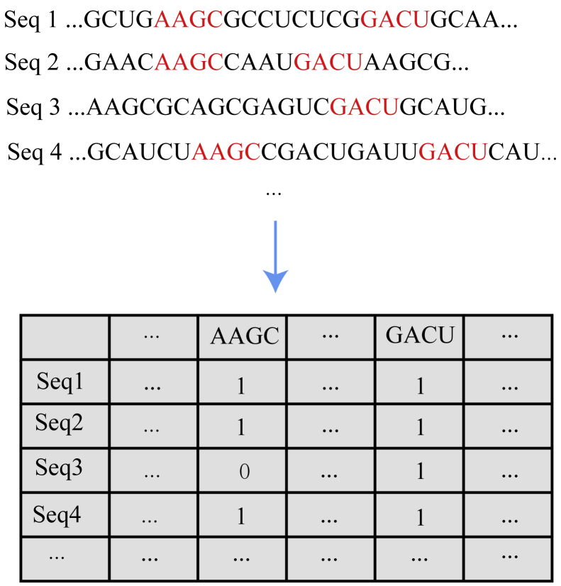
FGK are subjects and whose lengths over a threshold is an attribute clause which modifies the subjects. We can map each FGK sub-sequence into a column of the table as shown in Figure 5.

• (3)Utilize the frequent k-mer sub-sequence set as features to generate vectors.

Figure 5.

The Transformation from the Original Samples to 0–1 Sequences

First of all, we define the following functions:

$$c\left(S_i,Fk{M}_j\right)=\{\begin{array}{cc}1,& ifFk{M}_{j}exactlymatches{S}_i\\ 0,& Otherwise\end{array}$$ (Equation 6)

$$\varphi \left(S_i\right)=\left(\begin{array}{c}c\left(S_i,Fk{M}_1\right)\\ c\left(S_i,Fk{M}_2\right)\\ \begin{array}{c}\dots \\ c\left(S_i,Fk{M}_n\right)\end{array}\end{array}\right).$$ (Equation 7)

Here, ${\text{S}}_{\text{i}}$ denotes the sequence that is predicted, and ${\text{FkM}}_{\text{j}}$ denotes the j-element of the frequent k-mer sub-sequence set. As you can see from the function in Equation 6, we define a function $\text{c}$, which compares the predicted sequence ${\text{S}}_{\text{i}}$ and the j-element of the frequent k-mer sequence set, and we discriminate the perfect matching between ${\text{S}}_{\text{i}}$ and ${\text{FkM}}_{\text{j}}$ using 1 and 0 otherwise. After this procedure, we map the sequence ${\text{S}}_{\text{i}}$ using the function $\varphi$ to a 0–1 vector as shown in the function in Equation 7.

Linear Predictive Model

Although a huge amount of literature is related to classification methods such as SVM^21,52,54, 55, 56, 57, 58, 59, 60, 61, 62 and RF,^5,47, 48, 49, 50 as we can see from the feature representation algorithm of RNA sample, a series of sparse data is produced. Therefore, the need to deal with a large amount of sparse data is imperative. The linear predictive model is a linear classifier for processing a large amount of sparse data with a large number of examples and features. It is a general term for supervised models, including LR, SVM, and support vector regression (SVR). In this study, we used the packages LIBSVM⁶³ and LIBLINEAR.⁶⁴ They support the multiple types of linear classifiers that we mentioned earlier. In this study, we used LR and achieved a good result. LR uses the optimal decision boundary to construct regression formula and fitted parameter sets. The main idea is as follows:

• 1.Construct the prediction function ${\text{h}}_{\text{θ}}$, where$\text{ θ }$represents the parameter sets of eigenvalue $\text{X}$.

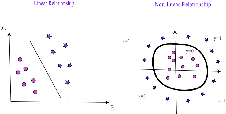
As far as we know, ${\text{h}}_{\text{θ}}$could have a linear relationship or non-linear relationship with $\text{X}$, as we can see from Figure 6. Normally, we can represent the linear relationship between ${\text{h}}_{\text{θ}}$and $\text{X}$ using the formula

$$h_{\theta }\left(x\right)=g\left({\theta }_0+{\theta }_1{x}_1+{\theta }_2{x}_2\right)$$ (Equation 8)

and the non-linear relationship using the formula

$$h_{\theta }\left(x\right)=g\left({\theta }_0+{\theta }_1{x}_1+{\theta }_2{x}_2+{\theta }_3{x}_1^2+{\theta }_4{x}_2^2\right).$$ (Equation 9)

In linear programming, the idea of cost function is to minimize the difference of predictive result ${\text{h}}_{\text{θ}}$and actual $\text{y}$; i.e.,

$$J\left(\theta \right)=\frac{1}{m}\sum _{i=1}^m\frac{1}{2}{\left(h_{\theta }\left(x^{\left(i\right)}\right)-y^{\left(i\right)}\right)}^2.$$ (Equation 10)

Then in LR, we can represent $J\left(\theta \right)$ as:

$$J\left(\theta \right)=\frac{1}{m}\sum _{i=1}^{m}Cost\left(h_{\theta }\left(x^{\left(i\right)}\right),y^{\left(i\right)}\right).$$ (Equation 11)

• 2.Use gradient descent to calculate the maximum of $J\left(\theta \right)$.

Figure 6.

The Linear and Non-linear Relationships between ${\text{h}}_{\text{θ}}$and $\text{X}$

For details, see the Linear Predictive Model section in Materials and Methods.

We can achieve the maximum of $\text{J}\left(\text{θ}\right)$ through fitting parameters using the gradient of the function. For simplicity, we can consider the following cost function

$$J\left(\theta \right)=\frac{1}{m}\sum _{i=1}^{m}Cost\left(h_{\theta }\left(x^{\left(i\right)}\right),y^{\left(i\right)}\right)$$ (Equation 12)

$$Cost\left(h_{\theta }\left(x\right),y\right)=\{\begin{array}{c}-\log \left(h_{\theta }\left(x\right)\right)ify=1\\ -\log \left(1-h_{\theta }\left(x\right)\right)ify=0\end{array}$$ (Equation 13)

and we can renew the parameter ${\text{θ}}_{\text{j}}\text{:}={\text{θ}}_{\text{j}}+\text{α}\left(\partial \text{J}\left(\text{θ}\right)/\partial {\text{θ}}_{\text{j}}\right)$; that is,

$${\theta }_j:={\theta }_j-\alpha \sum _{i=1}^m\left(h_{\theta }\left(x^{\left(i\right)}\right)-y^{\left(i\right)}\right)x_j^{\left(i\right)}.$$ (Equation 14)

Author Contributions

Y.Z. conceived the project, designed the experiments, and edited the final version of the paper. H.L. performed the experiment. X.S. wrote the paper and drafted the figures. H.P. contributed to materials and data analysis.

Conflicts of Interest

The authors declare no competing interests.

References

- 1.Acharjee A., Kloosterman B., Visser R.G.F., Maliepaard C. Integration of multi-omics data for prediction of phenotypic traits using random forest. BMC Bioinformatics. 2016;17(Suppl 5):180. doi: 10.1186/s12859-016-1043-4. [DOI] [PMC free article] [PubMed] [Google Scholar]
- 2.Belk A., Xu Z.Z., Carter D.O., Lynne A., Bucheli S., Knight R., Metcalf J.L. Microbiome data accurately predicts the postmortem interval using random forest regression models. Genes (Basel) 2018;9:E104. doi: 10.3390/genes9020104. [DOI] [PMC free article] [PubMed] [Google Scholar]
- 3.Cantara W.A., Crain P.F., Rozenski J., McCloskey J.A., Harris K.A., Zhang X., Vendeix F.A., Fabris D., Agris P.F. The RNA modification database, RNAMDB: 2011 update. Nucleic Acids Res. 2011;39:D195–D201. doi: 10.1093/nar/gkq1028. [DOI] [PMC free article] [PubMed] [Google Scholar]
- 4.Desrosiers R., Friderici K., Rottman F. Identification of methylated nucleosides in messenger RNA from Novikoff hepatoma cells. Proc. Natl. Acad. Sci. USA. 1974;71:3971–3975. doi: 10.1073/pnas.71.10.3971. [DOI] [PMC free article] [PubMed] [Google Scholar]
- 5.Roundtree I.A., Evans M.E., Pan T., He C. Dynamic RNA modifications in gene expression regulation. Cell. 2017;169:1187–1200. doi: 10.1016/j.cell.2017.05.045. [DOI] [PMC free article] [PubMed] [Google Scholar]
- 6.Wang X., Lu Z., Gomez A., Hon G.C., Yue Y., Han D., Fu Y., Parisien M., Dai Q., Jia G. N6-methyladenosine-dependent regulation of messenger RNA stability. Nature. 2014;505:117–120. doi: 10.1038/nature12730. [DOI] [PMC free article] [PubMed] [Google Scholar]
- 7.Jia G., Fu Y., Zhao X., Dai Q., Zheng G., Yang Y., Yi C., Lindahl T., Pan T., Yang Y.G., He C. N6-methyladenosine in nuclear RNA is a major substrate of the obesity-associated FTO. Nat. Chem. Biol. 2011;7:885–887. doi: 10.1038/nchembio.687. [DOI] [PMC free article] [PubMed] [Google Scholar]
- 8.Nilsen T.W. Molecular biology. Internal mRNA methylation finally finds functions. Science. 2014;343:1207–1208. doi: 10.1126/science.1249340. [DOI] [PubMed] [Google Scholar]
- 9.Meyer K.D., Saletore Y., Zumbo P., Elemento O., Mason C.E., Jaffrey S.R. Comprehensive analysis of mRNA methylation reveals enrichment in 3′ UTRs and near stop codons. Cell. 2012;149:1635–1646. doi: 10.1016/j.cell.2012.05.003. [DOI] [PMC free article] [PubMed] [Google Scholar]
- 10.Dominissini D., Moshitch-Moshkovitz S., Schwartz S., Salmon-Divon M., Ungar L., Osenberg S., Cesarkas K., Jacob-Hirsch J., Amariglio N., Kupiec M. Topology of the human and mouse m6A RNA methylomes revealed by m6A-seq. Nature. 2012;485:201–206. doi: 10.1038/nature11112. [DOI] [PubMed] [Google Scholar]
- 11.Linder B., Grozhik A.V., Olarerin-George A.O., Meydan C., Mason C.E., Jaffrey S.R. Single-nucleotide-resolution mapping of m6A and m6Am throughout the transcriptome. Nat. Methods. 2015;12:767–772. doi: 10.1038/nmeth.3453. [DOI] [PMC free article] [PubMed] [Google Scholar]
- 12.Meyer K.D., Jaffrey S.R. Rethinking m6A readers, writers, and erasers. Annu. Rev. Cell Dev. Biol. 2017;33:319–342. doi: 10.1146/annurev-cellbio-100616-060758. [DOI] [PMC free article] [PubMed] [Google Scholar]
- 13.Schwartz S., Agarwala S.D., Mumbach M.R., Jovanovic M., Mertins P., Shishkin A., Tabach Y., Mikkelsen T.S., Satija R., Ruvkun G. High-resolution mapping reveals a conserved, widespread, dynamic mRNA methylation program in yeast meiosis. Cell. 2013;155:1409–1421. doi: 10.1016/j.cell.2013.10.047. [DOI] [PMC free article] [PubMed] [Google Scholar]
- 14.Chen W., Feng P., Ding H., Lin H., Chou K.C. iRNA-Methyl: identifying N(6)-methyladenosine sites using pseudo nucleotide composition. Anal. Biochem. 2015;490:26–33. doi: 10.1016/j.ab.2015.08.021. [DOI] [PubMed] [Google Scholar]
- 15.Chen W., Feng P., Ding H., Lin H. Identifying N 6-methyladenosine sites in the Arabidopsis thaliana transcriptome. Mol. Genet. Genomics. 2016;291:2225–2229. doi: 10.1007/s00438-016-1243-7. [DOI] [PubMed] [Google Scholar]
- 16.Chen W., Tang H., Lin H. MethyRNA: a web server for identification of N6-methyladenosine sites. J. Biomol. Struct. Dyn. 2017;35:683–687. doi: 10.1080/07391102.2016.1157761. [DOI] [PubMed] [Google Scholar]
- 17.Chen W., Feng P., Yang H., Ding H., Lin H., Chou K.C. iRNA-3typeA: identifying three types of modification at RNA’s adenosine sites. Mol. Ther. Nucleic Acids. 2018;11:468–474. doi: 10.1016/j.omtn.2018.03.012. [DOI] [PMC free article] [PubMed] [Google Scholar]
- 18.Chen W., Ding H., Zhou X., Lin H., Chou K.C. iRNA(m6A)-PseDNC: identifying N6-methyladenosine sites using pseudo dinucleotide composition. Anal. Biochem. 2018;561–562:59–65. doi: 10.1016/j.ab.2018.09.002. [DOI] [PubMed] [Google Scholar]
- 19.Feng P., Ding H., Yang H., Chen W., Lin H., Chou K.C. iRNA-PseColl: identifying the occurrence sites of different RNA modifications by incorporating collective effects of nucleotides into PseKNC. Mol. Ther. Nucleic Acids. 2017;7:155–163. doi: 10.1016/j.omtn.2017.03.006. [DOI] [PMC free article] [PubMed] [Google Scholar]
- 20.Chen J., Long R., Wang X.L., Liu B., Chou K.C. dRHP-PseRA: detecting remote homology proteins using profile-based pseudo protein sequence and rank aggregation. Sci. Rep. 2016;6:32333. doi: 10.1038/srep32333. [DOI] [PMC free article] [PubMed] [Google Scholar]
- 21.Liu B., Zhang D., Xu R., Xu J., Wang X., Chen Q., Dong Q., Chou K.C. Combining evolutionary information extracted from frequency profiles with sequence-based kernels for protein remote homology detection. Bioinformatics. 2014;30:472–479. doi: 10.1093/bioinformatics/btt709. [DOI] [PMC free article] [PubMed] [Google Scholar]
- 22.Zou Q., Guo J., Ju Y., Wu M., Zeng X., Hong Z. Improving tRNAscan-SE annotation results via ensemble classifiers. Mol. Inform. 2015;34:761–770. doi: 10.1002/minf.201500031. [DOI] [PubMed] [Google Scholar]
- 23.Chen W., Xing P., Zou Q. Detecting N6-methyladenosine sites from RNA transcriptomes using ensemble support vector machines. Sci. Rep. 2017;7:40242. doi: 10.1038/srep40242. [DOI] [PMC free article] [PubMed] [Google Scholar]
- 24.Wei L., Chen H., Su R. M6APred-EL: a sequence-based predictor for identifying N6-methyladenosine sites using ensemble learning. Mol. Ther. Nucleic Acids. 2018;12:635–644. doi: 10.1016/j.omtn.2018.07.004. [DOI] [PMC free article] [PubMed] [Google Scholar]
- 25.Wei L., Xing P., Zeng J., Chen J., Su R., Guo F. Improved prediction of protein-protein interactions using novel negative samples, features, and an ensemble classifier. Artif. Intell. Med. 2017;83:67–74. doi: 10.1016/j.artmed.2017.03.001. [DOI] [PubMed] [Google Scholar]
- 26.Wei L., Wan S., Guo J., Wong K.K. A novel hierarchical selective ensemble classifier with bioinformatics application. Artif. Intell. Med. 2017;83:82–90. doi: 10.1016/j.artmed.2017.02.005. [DOI] [PubMed] [Google Scholar]
- 27.Liu Y., Zeng X., He Z., Zou Q. Inferring microRNA-disease associations by random walk on a heterogeneous network with multiple data sources. IEEE/ACM Trans. Comput. Biol. Bioinformatics. 2017;14:905–915. doi: 10.1109/TCBB.2016.2550432. [DOI] [PubMed] [Google Scholar]
- 28.Zhang J., Zhang Z., Chen Z., Deng L. Integrating multiple heterogeneous networks for novel lncRNA-disease association inference. IEEE/ACM Trans. Comput. Biol. Bioinform. 2019;16:396–406. doi: 10.1109/TCBB.2017.2701379. [DOI] [PubMed] [Google Scholar]
- 29.Tang W., Wan S., Yang Z., Teschendorff A.E., Zou Q. Tumor origin detection with tissue-specific miRNA and DNA methylation markers. Bioinformatics. 2018;34:398–406. doi: 10.1093/bioinformatics/btx622. [DOI] [PubMed] [Google Scholar]
- 30.Moridikia A., Mirzaei H., Sahebkar A., Salimian J. MicroRNAs: potential candidates for diagnosis and treatment of colorectal cancer. J. Cell. Physiol. 2018;233:901–913. doi: 10.1002/jcp.25801. [DOI] [PubMed] [Google Scholar]
- 31.Zhao R., Zhang Y., Zhang X., Yang Y., Zheng X., Li X., Liu Y., Zhang Y. Exosomal long noncoding RNA HOTTIP as potential novel diagnostic and prognostic biomarker test for gastric cancer. Mol. Cancer. 2018;17:68. doi: 10.1186/s12943-018-0817-x. [DOI] [PMC free article] [PubMed] [Google Scholar]
- 32.Chen J., Liu H., Yang J., Chou K.C. Prediction of linear B-cell epitopes using amino acid pair antigenicity scale. Amino Acids. 2007;33:423–428. doi: 10.1007/s00726-006-0485-9. [DOI] [PubMed] [Google Scholar]
- 33.Chou K.-C. Prediction of signal peptides using scaled window. Peptides. 2001;22:1973–1979. doi: 10.1016/s0196-9781(01)00540-x. [DOI] [PubMed] [Google Scholar]
- 34.Liu B., Wang S., Long R., Chou K.C. iRSpot-EL: identify recombination spots with an ensemble learning approach. Bioinformatics. 2017;33:35–41. doi: 10.1093/bioinformatics/btw539. [DOI] [PubMed] [Google Scholar]
- 35.Liu L.M., Xu Y., Chou K.C. iPGK-PseAAC: identify lysine phosphoglycerylation sites in proteins by incorporating four different tiers of amino acid pairwise coupling information into the general PseAAC. Med. Chem. 2017;13:552–559. doi: 10.2174/1573406413666170515120507. [DOI] [PubMed] [Google Scholar]
- 36.Liu B., Yang F., Huang D.S., Chou K.C. iPromoter-2L: a two-layer predictor for identifying promoters and their types by multi-window-based PseKNC. Bioinformatics. 2018;34:33–40. doi: 10.1093/bioinformatics/btx579. [DOI] [PubMed] [Google Scholar]
- 37.Liu B., Yang F., Chou K.C. 2L-piRNA: a two-layer ensemble classifier for identifying piwi-interacting RNAs and their function. Mol. Ther. Nucleic Acids. 2017;7:267–277. doi: 10.1016/j.omtn.2017.04.008. [DOI] [PMC free article] [PubMed] [Google Scholar]
- 38.Ehsan A., Mahmood K., Khan Y.D., Khan S.A., Chou K.C. A novel modeling in mathematical biology for classification of signal peptides. Sci. Rep. 2018;8:1039. doi: 10.1038/s41598-018-19491-y. [DOI] [PMC free article] [PubMed] [Google Scholar]
- 39.Song J., Wang Y., Li F., Akutsu T., Rawlings N.D., Webb G.I., Chou K.C. iProt-Sub: a comprehensive package for accurately mapping and predicting protease-specific substrates and cleavage sites. Brief. Bioinform. 2019;20:638–658. doi: 10.1093/bib/bby028. [DOI] [PMC free article] [PubMed] [Google Scholar]
- 40.Lin H., Deng E.Z., Ding H., Chen W., Chou K.C. iPro54-PseKNC: a sequence-based predictor for identifying sigma-54 promoters in prokaryote with pseudo k-tuple nucleotide composition. Nucleic Acids Res. 2014;42:12961–12972. doi: 10.1093/nar/gku1019. [DOI] [PMC free article] [PubMed] [Google Scholar]
- 41.Xu Y., Shao X.J., Wu L.Y., Deng N.Y., Chou K.C. iSNO-AAPair: incorporating amino acid pairwise coupling into PseAAC for predicting cysteine S-nitrosylation sites in proteins. PeerJ. 2013;1:e171. doi: 10.7717/peerj.171. [DOI] [PMC free article] [PubMed] [Google Scholar]
- 42.Li W.C., Deng E.Z., Ding H., Chen W., Lin H. iORI-PseKNC: a predictor for identifying origin of replication with pseudo k-tuple nucleotide composition. Chemometr. Intell. Lab. Syst. 2015;141:100–106. [Google Scholar]
- 43.Feng C.Q., Zhang Z.Y., Zhu X.J., Lin Y., Chen W., Tang H., Lin H. iTerm-PseKNC: a sequence-based tool for predicting bacterial transcriptional terminators. Bioinformatics. 2019;35:1469–1477. doi: 10.1093/bioinformatics/bty827. [DOI] [PubMed] [Google Scholar]
- 44.Chen W., Lv H., Nie F., Lin H. i6mA-Pred: identifying DNA N6-methyladenine sites in the rice genome. Bioinformatics. 2019;35:2796–2800. doi: 10.1093/bioinformatics/btz015. [DOI] [PubMed] [Google Scholar]
- 45.Chen W., Yang H., Feng P., Ding H., Lin H. iDNA4mC: identifying DNA N4-methylcytosine sites based on nucleotide chemical properties. Bioinformatics. 2017;33:3518–3523. doi: 10.1093/bioinformatics/btx479. [DOI] [PubMed] [Google Scholar]
- 46.Feng P., Yang H., Ding H., Lin H., Chen W., Chou K.C. iDNA6mA-PseKNC: Identifying DNA N6-methyladenosine sites by incorporating nucleotide physicochemical properties into PseKNC. Genomics. 2019;111:96–102. doi: 10.1016/j.ygeno.2018.01.005. [DOI] [PubMed] [Google Scholar]
- 47.Adams J.M., Cory S. Modified nucleosides and bizarre 5′-termini in mouse myeloma mRNA. Nature. 1975;255:28–33. doi: 10.1038/255028a0. [DOI] [PubMed] [Google Scholar]
- 48.Naue J., Hoefsloot H.C.J., Mook O.R.F., Rijlaarsdam-Hoekstra L., van der Zwalm M.C.H., Henneman P., Kloosterman A.D., Verschure P.J. Chronological age prediction based on DNA methylation: Massive parallel sequencing and random forest regression. Forensic Sci. Int. Genet. 2017;31:19–28. doi: 10.1016/j.fsigen.2017.07.015. [DOI] [PubMed] [Google Scholar]
- 49.Sarkar R.K., Rao A.R., Meher P.K., Nepolean T., Mohapatra T. Evaluation of random forest regression for prediction of breeding value from genomewide SNPs. J. Genet. 2015;94:187–192. doi: 10.1007/s12041-015-0501-5. [DOI] [PubMed] [Google Scholar]
- 50.Svetnik V., Liaw A., Tong C., Culberson J.C., Sheridan R.P., Feuston B.P. Random forest: a classification and regression tool for compound classification and QSAR modeling. J. Chem. Inf. Comput. Sci. 2003;43:1947–1958. doi: 10.1021/ci034160g. [DOI] [PubMed] [Google Scholar]
- 51.Zhang M., Sun J.W., Liu Z., Ren M.W., Shen H.B., Yu D.J. Improving N(6)-methyladenosine site prediction with heuristic selection of nucleotide physical-chemical properties. Anal. Biochem. 2016;508:104–113. doi: 10.1016/j.ab.2016.06.001. [DOI] [PubMed] [Google Scholar]
- 52.Zhou Y., Zeng P., Li Y.H., Zhang Z., Cui Q. SRAMP: prediction of mammalian N6-methyladenosine (m6A) sites based on sequence-derived features. Nucleic Acids Res. 2016;44:e91. doi: 10.1093/nar/gkw104. [DOI] [PMC free article] [PubMed] [Google Scholar]
- 53.Luo G.Z., MacQueen A., Zheng G., Duan H., Dore L.C., Lu Z., Liu J., Chen K., Jia G., Bergelson J., He C. Unique features of the m6A methylome in Arabidopsis thaliana. Nat. Commun. 2014;5:5630. doi: 10.1038/ncomms6630. [DOI] [PMC free article] [PubMed] [Google Scholar]
- 54.Chen X., Yan C.C., Zhang X., You Z.H., Deng L., Liu Y., Zhang Y., Dai Q. WBSMDA: within and between score for miRNA-disease association prediction. Sci. Rep. 2016;6:21106. doi: 10.1038/srep21106. [DOI] [PMC free article] [PubMed] [Google Scholar]
- 55.Tang H., Chen W., Lin H. Identification of immunoglobulins using Chou’s pseudo amino acid composition with feature selection technique. Mol. Biosyst. 2016;12:1269–1275. doi: 10.1039/c5mb00883b. [DOI] [PubMed] [Google Scholar]
- 56.Yang H., Tang H., Chen X.X., Zhang C.J., Zhu P.P., Ding H., Chen W., Lin H. Identification of secretory proteins in Mycobacterium tuberculosis using pseudo amino acid composition. BioMed Res. Int. 2016;2016:5413903. doi: 10.1155/2016/5413903. [DOI] [PMC free article] [PubMed] [Google Scholar]
- 57.Lin H., Liang Z.Y., Tang H., Chen W. Identifying sigma70 promoters with novel pseudo nucleotide composition. IEEE/ACM Trans. Comput. Biol. Bioinform. 2019;16:1316–1321. doi: 10.1109/TCBB.2017.2666141. [DOI] [PubMed] [Google Scholar]
- 58.Liu B., Fang L., Liu F., Wang X., Chen J., Chou K.C. Identification of real microRNA precursors with a pseudo structure status composition approach. PLoS ONE. 2015;10:e0121501. doi: 10.1371/journal.pone.0121501. [DOI] [PMC free article] [PubMed] [Google Scholar]
- 59.Xiao Y., Zhang J., Deng L. Prediction of lncRNA-protein interactions using HeteSim scores based on heterogeneous networks. Sci. Rep. 2017;7:3664. doi: 10.1038/s41598-017-03986-1. [DOI] [PMC free article] [PubMed] [Google Scholar]
- 60.Lai H.Y., Chen X.X., Chen W., Tang H., Lin H. Sequence-based predictive modeling to identify cancerlectins. Oncotarget. 2017;8:28169–28175. doi: 10.18632/oncotarget.15963. [DOI] [PMC free article] [PubMed] [Google Scholar]
- 61.Chou K.C., Cai Y.D. Using functional domain composition and support vector machines for prediction of protein subcellular location. J. Biol. Chem. 2002;277:45765–45769. doi: 10.1074/jbc.M204161200. [DOI] [PubMed] [Google Scholar]
- 62.Cai Y.D., Zhou G.P., Chou K.C. Support vector machines for predicting membrane protein types by using functional domain composition. Biophys. J. 2003;84:3257–3263. doi: 10.1016/S0006-3495(03)70050-2. [DOI] [PMC free article] [PubMed] [Google Scholar]
- 63.Chang C.C., Lin C.J. LIBSVM: a library for support vector machines. ACM Trans. Intell. Syst. Technol. 2011;2:27. [Google Scholar]
- 64.Fan R.E., Chang K.-W., Hsieh C.-J., Wang X.-R., Lin C.-J. LIBLINEAR: a library for large linear classification. J. Mach. Learn. Res. 2008;9:1871–1874. [Google Scholar]