Estimation of model accuracy in CASP13

Abstract

Methods to reliably estimate the accuracy of 3D models of proteins are both a fundamental part of most protein folding pipelines and important for reliable identification of the best models when multiple pipelines are used. Here, we describe the progress made from CASP12 to CASP13 in the field of estimation of model accuracy (EMA) as seen from the progress of the most successful methods in CASP13. We show small but clear progress, i.e. several methods perform better than the best methods from CASP12 when tested on CASP13 EMA targets. Some progress is driven by applying deep learning and residue-residue contacts to model accuracy prediction. We show that the best EMA methods select better models than the best servers in CASP13, but that there exists a great potential to improve this further. Also, according to the evaluation criteria based on local similarities, such as lDDT and CAD, it is now clear that single model accuracy methods perform relatively better than consensus-based methods.

Introduction

Estimation of model accuracy (EMA) is vital for both selecting structural models in protein structure prediction and using them appropriately in biomedical research. Many of EMA (or quality assessment (QA)) methods^1–5 have been developed to tackle this problem. In terms of input, EMA methods can be classified as single-model methods^3,5–7 and multi-model (or consensus) methods^8,9. The former takes a single structural model as input to predict its accuracy, while the latter uses multiple structural models of a protein as input to estimate their accuracy, often leveraging the similarity between the models. In terms of output, EMA methods can be categorized as global accuracy assessment methods^10,11 and local accuracy assessment methods¹², see Table I. The global methods predict a single global score (e.g. GDT-TS score) measuring the global accuracy of a whole model, whereas the local methods estimate the local accuracy (e.g. the distance deviation from the native position) for each residue in a model. The vast majority of local accuracy methods also produce a global estimate of the accuracy. This is often done by using the average local accuracy.

Table I:

overview of methods discussed in this paper and the way they were developed.

Method	Local/Global	Inputs	Sequence features	Structure features	Predicted Features	Target Function	Machine Learning method
FaeNNz	Local (Global is avg. Local)	Model and full length target sequence		Statistical Potentials of Mean Force + Distance Constraints from Templates + Solvent Acc.	Sec. Str and Surface Area	LDDT (local)	Multi-Layer Perceptron
ModFOLD7	Local (Global is sum of local)	Model and full length target sequence	PSSM	Pairwise comparisons of generated reference models, residue contacts	Contacts, Sec.Str and Disorder	S-score (local)	Multi-Layer Perceptron
ModFOLD7_cor	Local and optimised composite global score	Model and full length target sequence	PSSM	Pairwise comparisons of generated reference models, residue contacts	Contacts, Sec.Str and Disorder	lDDT (local) GDT_TS (global)	Multi-Layer Perceptron
ModFOLD7_rank	Local and optimised composite global score	Model and full length target sequence	PSSM	Pairwise comparisons of generated reference models, residue contacts	Contacts, Sec.Str and Disorder	S-score (local) GDT_TS (global)	Multi-Layer Perceptron
ProQ2	Local (Global is sum of local)	Profile+Model+Predictions	PSSM	Atom Contacts, Residue Contacts	Sec.Str and Surface Area	S-score (local)	Linear SVM
ProQ3	Local (Global is sum of local)	Profile+Model+Predictions+Energies	PSSM	ProQ2+Energy terms	Sec.Str and Surface Area	S-score (local)	Linear SVM
ProQ3D	Local (Global is sum of local)	Profile+Structure+Predictions+Energies	PSSM	See ProQ3	See ProQ3	S-score (local)	Multi-Layer Perceptron
ProQ3D-TM	Local (Global is sum of local)	Profile+Model+Predictions+Energies	PSSM	See ProQ3	See ProQ3	TM-score (local)	Multi-Layer Perceptron
ProQ3D-lDDT	Local (Global is sum of local)	Profile+Model+Predictions+Energies	PSSM	See ProQ3	See ProQ3	lDDT(local)	Multi-Layer Perceptron
ProQ3D-CAD	Local (Global is sum of local)	Profile+Model+Predictions+Energies	PSSM	See ProQ3	See ProQ3	CAD-score (local)	Multi-Layer Perceptron
ProQ4 (ProQ4)	Local (Global is sum of local)	Profile+ DSSP	PSSM	DSSP (sec. Str and surface area)	Internally DSSP.	lDDT(local)	Deep Network
SART_G	Global	Model+Predictions+Energies		Statistical Potentials + Solvent Acc + Sec. Str + Residue Contact	Sec. Str, Solvent Acc and Residue Contact	GDT_TS	Linear Regression
SART_L	Local	Model+Predictions+Energies		Statistical Potentials + Solvent Acc + Sec. Str + Residue Contact	Sec. Str, Solvent Acc and Residue Contact	S-score	Linear Regression
SARTclust_G	Global	Model+Predictions+Energies		Statistical Potentials + Solvent Acc + Sec. Str + Residue Contact	Sec. Str, Solvent Acc and Residue Contact	GDT_TS	Linear Regression
VoroMQA-A, VoroMQA-B	Local and global	Model	Not used	Voronoi tessellation-based contact areas.	Not used	Not used	Statistical potential
MULTICOM-CLUSTER	Global	Model and full-length sequence	Not used	Secondary structure, Solvent accessibility, residue contacts	Contacts, Sec.Str, Surface Area and Structural scores	GDT_TS (global)	Deep Network+ensemble
MULTICOM- CONSTRUCT	Global	Model and full-length sequence	Not used	Secondary structure, Solvent accessibility, residue contacts	Contacts, Sec.Str, Surface Area and Structural scores	GDT_TS (global)	Deep Network+ensemble
MULTICOM NOVEL	Local (Global is sum of local)	Model and full-length sequence	PSSM, Amino acid encoding	Secondary structure, Solvent accessibility, Energy terms	Disorder, Sec.Str and Surface Area	S-score (local) and GDT_TS (global)	Deep Network

Different EMA methods utilize different descriptions of the models. Historically, EMA methods were often divided into single and consensus methods. Here, single methods only use a single model and predicts the accuracy of that model (or regions of that model), while consensus methods compared a set of models and (often) assumed that the more similar they were the more likely they were to be correct. In earlier CASPs a category of “quasi-single” methods also existed. These methods do not require a set of models, as for the consensus methods, instead they compare the model with a set of internally generated models, assuming that the more similar the model is to the internally generated models the better it is. Now, many methods combine many of the methods making it hard to exactly classify each method, but we have tried to describe the most important features of all our methods in Table I.

Due to its importance, EMA became an independent category in the 7’th Critical Assessment of Techniques for Protein Structure Prediction (CASP7) in 2006 and has remained a major open challenge of CASP since then. In CASP13, 52 groups including 41 automated server predictors from around the world participated in the EMA experiment, which represented a variety of state-of-the-art methods in the field. In this work, we summarized the results of the EMA predictors from six top-performing labs in the CASP13 experiment. We analyzed the strengths and weaknesses of these methods. We investigated the progress in the field from CASP12 to CASP13 and identified the major challenges to be overcome in the future.

We show that there has been measurable progress since CASP12. Although direct comparisons are difficult, as the targets and underlying methods that generate the targets change between CASP seasons, it is clear that progress has been made as novel methods outperform the best methods in CASP12. Further, we show that the best EMA methods slightly outperform the best servers when it comes to selecting one model per target.

Methods

A summary of all methods can be found in Table I. Below is a brief description of the CASP13 predictors of the six top-performing groups.

Cheng group - MULTICOM_CLUSTER, MULTICOM-CONSTRUCT, MULTICOM-NOVEL

We benchmarked three new deep learning-based EMA servers (MULTICOM_CLUSTER, MULTICOM-CONSTRUCT, and MULTICOM-NOVEL) in CASP13.

MULTICOM_CLUSTER and MULTICOM-CONSTRUCT servers are the consensus-based methods for estimating the accuracy of protein structural models. Different from the linear combination of scores from multiple quality assessment methods in CASP11 and CASP12 ⁴, in CASP13, we applied deep learning and ensemble techniques to integrate a wide variety of accuracy scores and inter-residue contact predictions for predicting the global accuracy of models ¹³. Given a pool of models, the methods first use SCWRL¹⁴ to repack their side-chains to make them consistent. They then generate several 3D accuracy scores for each model by using 9 single-model QA methods (i.e. SBROD¹⁵, OPUS_PSP¹⁶, RF_CB_SRS_OD¹⁷, Rwplus¹⁸, DeepQA¹⁹, ProQ2⁶, ProQ3²⁰, Dope²¹ and Voronota²²) as well as three consensus-based QA methods (i.e. APOLLO²³, Pcons⁸, and ModFOLDclust2²⁴). In addition, they incorporate the novel 2D contact features, i.e. the percentage of predicted inter-residue contacts (i.e. top L/5 short-range, medium-range and long-range contacts predicted by DNCON2²⁵) existing in a model. Several 1D sequence features are also used to score models including the agreement between the secondary structure and solvent accessibility predicted from the protein sequence and the ones parsed from the models^26,27. The 1D, 2D and 3D features are used by the deep neural network method (DeepRank) to predict the global accuracy score (GDT_TS) of each model¹³. We used the predicted structures of CASP8–11 targets to train 10 deep neural networks via 10-fold cross-validation. All input features of each model are fed into the 10 pre-trained networks to generate 10 accuracy scores (GDT_TS score). For MULTICOM-CONSTRUCT server, the 10 accuracy scores are simply averaged as a final global score for each model. For MULTICOM_CLUSTER server, the 10 predicted accuracy scores are concatenated with the initial input features as the input for another deep neural network to predict the final accuracy score. Prior to CASP13, we benchmarked the performance of the two DeepRank-based methods on CASP12 targets along with our previous methods tested in the CASP11 and CASP12 that did not use deep learning and contact features⁴. The results showed that applying the deep neural network to integrate a set of accuracy scores and contact features achieved significant improvement over our methods used in CASP11 and CASP12 and outperformed all individual features on model ranking and selection.

MULTICOM-NOVEL server is a single-model accuracy assessment method that predicts the global accuracy and local (residual-specific) accuracy of protein structural models using a one-dimensional deep convolutional neural network (1D-CNN) ²⁸. The 1D-CNN was trained using a multi-task learning framework to predict the local scores of residues as well as the global accuracy (GDT-TS score) of a model. The objective of using the multi-task learning is to study whether global and local accuracy predictions can synergistically interact to improve the overall prediction performance. Given a structural model, the method first generates several residue-specific features and model-specific energies, which include (1) 20-digit amino acid encoding of each residue, (2) position specific scoring matrix (PSSM) profile of each residue derived from the multiple sequence alignment of the protein, (3) predicted disorder state of each residue, (4) the agreement between the secondary structure and solvent accessibility of each residue predicted from the sequence and the ones parsed from the model, (5) Rosetta energies of each residue used in the ProQ3²⁰, and (6) six global knowledge-based potentials or features of the model produced by ModelEvaluator²⁹, Dope²¹, RWplus¹⁷, Qprob³⁰, GOAP³¹, and Surface score¹⁹. For the local accuracy prediction, 1D-CNN uses the feature vector of length L (L: sequence length) as input to predict the S-score $S\left(d\right) =\frac{1}{1+{\left(\frac{d}{d_0}\right)}^2}$ for each residue in the model, where d is the distance deviation between the position of the residue in the model and that in the native structure and d₀ is set to 3.0 Å. The predicted S-score can be converted back to the distance d. For the global accuracy prediction, the global accuracy score of a model is derived by averaging the local accuracy predictions of residues directly using the formula $\frac{1}{L}{\sum }_{i=1}^L\frac{1}{1+{\left(\frac{d_i}{d_0}\right)}^2}$. The 1D-CNN was trained on the structural models of the single-domain protein targets of CASP8, 9, 10 and evaluated on the models of CASP11 and CASP12 targets. The source code of the method is available at https://github.com/multicom-toolbox/CNNQA.

Elofsson group - ProQ3D and ProQ4

Since the development of ProQres¹² for local predictions ProQ has been one of the best single-model EMA methods in CASP^1,20,32–34. All versions of ProQ has been developed continuously using the same strategy. Each residue in the protein model is described by a number of structural, sequence and prediction features. These features are then combined and compared to each other using different window sizes, including window sizes that includes the entire model. Finally a machine learning method is used to predict the error (accuracy) for each residue. ProQres, ProQ2, ProQ3 and ProQ3D are trained to predict the S-score, which correlates well with GDT_TS when the average S-score is used to estimate the global accuracy.

We participated with ProQ3D (in several versions) and ProQ4 in CASP13. In short, the different ProQ methods can be summarized as follows: Starting from ProQ2 developed by the Wallner lab⁶ we developed ProQ3 a few years ago by adding additional carefully tuned input features describing the accuracy of a protein model²⁰. ProQ3 was one of the best methods in CASP12^1,6,20. Both ProQ2 and ProQ3 uses a simple linear SVM to combine the many input features when estimating the accuracy of a model. In ProQ3D we replaced the simple SVM with a multilayer perceptron, thanks to the rapid improvement in training deep learning neural networks using GPUs ³⁵. A preliminary version of ProQ3D was used in CASP12 - but in CASP13 we used the final version which outperforms ProQ3 in almost all measures. In addition to the default version of ProQ3D which is trained to predict the S-score³⁶, we developed several versions that were trained to predict other model accuracy scores³⁷. These predictors are named ProQ3D-TM, ProQ3D-CAD and ProQ3D-lDDT.

In CASP13 we also used a preliminary version of ProQ4³⁸ - based on a distinct and novel approach. ProQ4 is using a simplified description of a protein model and an advanced deep learning approach. The target function is trained on the LDDT score (as ProQ3D-LDDT), while the protein model is described only by structural features given by DSSP^27,37 (dihedral angles, relative surface area, and secondary structure). Finally, the sequence is described by simple statistical features, such as entropy of each column in the multiple sequence alignment, and does not include predicted features as in ProQ3D. The underlying architecture is a deep convolutional network. However, the main difference between ProQ4 and other methods is that the network is trained using a comparative approach: at every iteration, two models from the same target are presented, and the network is trained to predict not only the scores of each model but also which one is better. Thereby it is possible to augment the data and to take advantage of the structure of the problem and it improves the ability to rank models.

ProQ3D is available as a web server and standalone at proq3.bioinfo.se. ProQ4 can be downloaded from github.com/ElofssonLab/ProQ4.

Han group - SART methods

We participated in CASP13 with 2 methods, SART (group name: “SASHAN”) and SARTclust (group name: “UOSHAN”). They are a new single model accuracy estimation method and a new clustering method, respectively. For details, see the CASP 13 abstracts at http://predictioncenter.org/casp13/doc/CASP13_Abstracts.pdf.

SART_G: Single model global accuracy score

For SART_G 10 features extracted from a protein model are linearly combined into the single model global accuracy score SART_G. The features of SART_G include 4 consistency-based terms and 6 statistical potential-based terms.

One important category of features is consistency-based terms between the predicted and the calculated values of the model in aspects of secondary structure, solvent accessibility and residue-residue contact. One consistency term is the 8 states-agreement between the predicted (by SSpro8_5.1 of SCRATCH³⁹ and the secondary structure calculated by DSSP²⁷) secondary structure of model. Solvent accessibility-based consistency terms include the binary agreement and Spearman correlation coefficient (R_SPE) between the predicted (by ACCpro_5.1 or ACCpro20_5.1 of SCRATCH) and the calculated solvent accessibility. Residue contact-based consistency term is calculated as number of residue pairs in the model which are in contact state and belong to the top 2×L (target protein sequence length) residue pairs with the highest predicted contact probability.

The other important category of features is statistical potential-based terms. They include 2 residue pair potentials, 2 torsion potential-related scores. The remaining 2 features are based on burial propensities of 20 amino acids and the buried state of 8 hydrophobic residues, respectively.

To enable comparisons between different proteins, most of the features are divided by n × L (for consistency-based terms) or Lⁿ (for statistical potential-based terms). Here, n is set differently for different terms using data of CASP7, CASP9 and CASP11.

SART_G is a linear combination of 10 features described above. Linear regression is performed between 10 features and GDT_TS^27,40 scores of 34337 CASP9 models.

SART_L: Single model-based local accuracy score

For SART_L 9 features are extracted from a sphere (radius 12 Å) centered on the residue of interest. The features of SART_L are similar to those of SART_G: 5 consistency-based terms and 4 statistical potential-based terms. The true distance, d, is converted to the S-score with threshold d₀=3.8Å, S = 1 / (1 + (d / d₀)²). Linear regression is done between 9 features and S-score⁴¹ calculated from 6818635 residues of 34337 CASP9 models. The per-residue distance deviation SART_L is calculated as SART_L = d₀ (1 / S-score - 1)^1/2. We put all SART_L>15Å to 15Å.

SARTclust

Our clustering method is based on the following idee: If we know a native structure, the accuracy of a protein model can be easily obtained by comparing the native structure to the model. In EMA a related method could be to identify the best model, i.e. the model closest to the native structure, and then estimate the accuracy of all models by comparing them with the best model. However, it is often difficult to identify the “best” model correctly and the quality of the best model might not be good enough. Given that our single model method SART_G is still not perfect and that the quality of the best model is sometimes low, our clustering method uses comparisons with several top-ranked models with diverse structural properties. According to benchmarks on CASP11 data, the appropriate number (n) of the chosen models was 11 for stage 1 and 21 for stage 2.

For calculating clustering-based global accuracy score SARTclust_G, a reference set composed of n top-ranked models is formed based on SART_G scores. A given model (to be assessed) is compared with each of n models in the reference set using TMscore^41,42, resulting in n GDT_TS scores. Finally, the clustering-based global accuracy score SARTclust_G is calculated as SART_G-weighted mean of n GDT_TS scores.

For calculating clustering-based local accuracy score SARTclust_L, the Cα distance (d) between the corresponding residues is computed after superposition of the given model and each of the models in the reference set using TMscore. The distances (d) are converted to the S-scores with threshold d₀=3.8Å. Next, SART_G-weighted mean (S_Weight) of n S scores is calculated. Finally, the per-residue distance deviation, SARTclust_L is calculated as SARTclust_L = d₀ (1/ S_Weight −1)^1/2. We put all SARTclust_L>15Å to 15Å.

The weighting scheme makes the different models contribute differently to the estimation of the given model’s accuracy according to their SART_G scores.

McGuffin group - ModFOLD7 methods

The ModFOLD7 server is the latest version of our web resource for the estimation of model accuracy (EMA) of 3D models of proteins^1,2,3, which combines the strengths of multiple pure-single and quasi-single model methods for improving prediction accuracy. For CASP13, our emphasis was on increasing the accuracy of per-residue assessments for single models, single model ranking and score consistency. Each model was considered individually using six previously described pure-single model methods: CDA³, SSA³, ProQ2⁴, ProQ2D⁵, ProQ3D⁵ and VoroMQA⁵. Additionally, reference 3D-models sets were generated using the IntFOLD5 server⁴³ and these were used to score models using four previously described quasi-single model methods: DBA³, MF5s³, MFcQs³ and ResQ⁷. Neural networks, specifically multilayer perceptrons (MLPs), were then used to combine the residue scores produced by the ten alternative scoring methods, resulting in a final consensus accuracy score for each residue in each model (Figure 1)

Figure 1:

Flow of data and processes for the ModFOLD7 method variants. The inputs at the top are simply a single 3D model and the target sequence. The target sequence was pre-processed by a number of different methods to produce predicted secondary structures, contacts, disorder and reference models. These data were then fed into the 10 different scoring methods to produce local scores. The local scores were then used as inputs to neural networks, which were then trained using either the S-score or the lDDT score as the target function. The mean local scores for each model were then taken to produce global scores from each input method. Combinations of these global scores were used to generate ModFOLD7_rank, ModFOLD7_cor and ModFOLD7 global scores

Component per-residue/local accuracy scoring methods:

The ModFOLD7 neural networks were trained using two separate target functions for each residue in a model: the superposition based S-score³⁶ used previously³ and the residue contact based lDDT score⁸. For the network trained using the lDDT score (ModFOLD7_res_lddt), the per-residue similarity scores were calculated using a simple multilayer perceptron (MLP). The MLP input consisted of a sliding window (size=5) of per-residue scores from all 10 of methods described above, and the output was a single accuracy score for each residue in the model (50 inputs, 25 hidden and 1 output). For the method trained with the S-score (ModFOLD7_res), the per-residue similarity scores were also calculated using an MLP with a sliding window (size=5) of per-residue scores, but this time only 7 of the 10 methods were used as inputs - all apart from the ProQ2, CDA and SSA scores (resulting in 35 inputs, 18 hidden and 1 output). The RSNNS package for R was used to construct the MLPs, which were trained using data derived from the evaluation of CASP11 & 12 server models versus native structures. The MLP output scores, s, for each residue were then converted back to a distance, d, using this formula:

d = 3.5√((1/s)−1).

Global scoring methods:

Global scores were calculated by taking the mean per-residue scores (the sum of the per-residue similarity scores divided by sequence lengths) for each of the 10 individual component methods, described above, plus the NN output from ModFOLD7_res and ModFOLD7_res_lddt. Furthermore, 3 additional quasi-single global model accuracy scores were generated for each model based on the original ModFOLDclust, ModFOLDclustQ and ModFOLDclust2 global scoring methods, which have been described previously⁹. Thus, we ended up with 15 alternative global QA scores, which could be combined in various ways in order to optimize for the different facets of the accuracy estimation problem. We registered three ModFOLD7 global scoring variants:

• The standard ModFOLD7 global score was simply the mean per-residue output score from ModFOLD7_res, which was found to have a good balance of performance both for correlations of predicted and observed scores and rankings of the top models.

• The ModFOLD7_cor global score variant ((MFcQs + DBA + ProQ3D + ResQ + ModFOLD7_res)/5) was found to be an optimal combination for producing good correlations with the observed scores, i.e. the predicted global accuracy scores should provide more linear correlations with the observed global accuracy scores.

• The ModFOLD7_rank global score variant ((CDA + SSA + VoroMQA + ModFOLD7_res + ModFOLD7res_lDDT)/5) was found to be an optimal combination for ranking, i.e. the top ranked models (top 1) should be closer to the highest accuracy, but the relationship between predicted and observed scores may not be linear.

The local scores of the ModFOLD7 and ModFOLD_rank variants used the output from the ModFOLD7_res NN, whereas the ModFOLD_cor variant used the local scores from the ModFOLD7_res_lddt NN. All three of the ModFOLD7 variants are freely available at: http://www.reading.ac.uk/bioinf/ModFOLD/ModFOLD7_form.html

ModFOLDclust2

The ModFOLDclust2 method⁹ is a leading clustering approach for both local and global 3D model accuracy estimation. The ModFOLDclust2 server which was tested during CASP13 was identical to that tested in the CASP9–12 experiments, and it, therefore, serves as a useful gauge against which to measure the progress of single model methods. ModFOLDclust2 can be run as an option via the older ModFOLD3 server at http://www.reading.ac.uk/bioinf/ModFOLD/ModFOLD_form_3_0.html. The software is also available to download as a standalone program at http://www.reading.ac.uk/bioinf/downloads/

Studer group - FaeNNz methods

FaeNNz is the working title of an improved version of QMEANDisCo, the default accuracy estimation method employed by the SWISS-MODEL homology modelling server⁴⁴. The method aims to efficiently calculate local per-residue accuracy estimates using one single structural model as input. As the global full model score, the average of per-residue scores has been submitted. As of writing this article, the method tested in CASP13 has been merged back into QMEANDisCo and will be described in full detail elsewhere [manuscript in preparation]. The implementation is accessible on the web (https://swissmodel.expasy.org/qmean) or as source code (https://git.scicore.unibas.ch/schwede/QMEAN).

FaeNNz is a composite scoring function mainly relying on knowledge-based statistical potentials of mean force ⁷ that are trained on a non-redundant set of experimentally determined protein structures. There are:

• Two Interaction Potentials: The first one assesses pairwise interactions between all chemically distinguishable heavy atoms, the second one only between Cβ atoms.

• Two Packing Potentials: The first one assesses the number of close heavy atoms around all chemically distinguishable heavy atoms, the second one only considers Cβ atoms.

• One Reduced Potential: Assesses pairwise interactions between a reduced representation of amino acids. Such a reduced representation is composed of the Cα position and a directional component constructed from backbone N, Cα and C positions.

• One Torsion Potential: The central φ/ψ angles of three consecutive amino acids are assessed given the identity of the full triplet.

Non-statistical potential terms include a clash score as defined for SCWRL3⁴⁵, the raw count of other residues within 15Å and solvent accessibility in Ų. They are complemented by the agreement of secondary structure and solvent accessibility predictions from the sequence (PSIPRED⁴⁶ / ACCPRO³⁹) with the actual outcome from the model coordinates.

Known structures thoroughly represent the structural variety of a protein family in many cases. If available, FaeNNz utilizes this information by employing an additional score, the DisCo (Distance Constraints) score that is constructed from templates homologous to the model in question that are found by HHblits⁴⁷. DisCo consists of Cα-Cα constraints for every residue pair, and the per-residue DisCo score is the averaged outcome of all constraints involving one residue.

The accuracy of DisCo is directly related to the structural similarity of the used templates to the native structure. To optimally exploit DisCo, particularly in combination with other terms that are independent from the template situation, the reliability of DisCo needs to be quantified. FaeNNz uses terms like sequence identity/ similarity (BLOSUM62) of found templates or the variance of pairwise distances used for constraint construction. They are passed to a subsequent machine learning step to optimally weigh the DisCo term with all other described components in order to get a final per-residue score.

All previously described components compose the input layer of a neural network trained to predict local lDDT scores⁴⁸. Amino acid specific biases for composite scores have been identified in previous work⁴⁹ and taken into account in the input layer by using “one-hot” encoding. Various network topologies and training parametrizations have been sampled using a 5-fold cross-validation (80% training / 20% test) on three data sets. (1) approximately 2 mio. per-residue data points extracted from models submitted from the CAMEO QE category⁵⁰ (2) approximately 2 mio. per-residue data points from models submitted from the CASP12 EMA category (3) a mixed set composed of a random selection of 50% from each of the first two. The cross validation of (3) has been constructed to maintain a valid cross validation when training on (3) but testing on (1)/(2). The finally used network has been trained on (3) and contains 3 hidden layers of width 20. It exhibited superior test performance compared to networks trained on (1)/ tested on (2) and vice versa. It also exhibited equal or better test performance as it has been observed for the raw cross-validation on (1) or (2) and thus successfully generalized data from different sources (Table II).

Table II:

Cross-validation performance of FaeNNz with final neural network topology/parametrization across different data-sets when predicting per-residue lDDT scores. Prediction results for all 5 validation sets in each cross-validation have been pooled together to estimate the performance in form of Pearson correlation and receiver operation characteristics (ROC) analysis. Data points with per-residue lDDT < 0.6 have been classified as “positive” in ROC analysis.

	Validation
	CAMEO		CASP12
Training	Pearson R	ROC AUC	Pearson R	ROC AUC
CASP12	0.841	0.917	0.836	0.937
CAMEO	0.887	0.940	0.812	0.934
Mixed	0.889	0.940	0.856	0.946

Venclovas group - VoroMQA methods

Two automated model accuracy estimation methods, VoroMQA-A and VoroMQA-B, employed the latest version of VoroMQA⁵, a method for the estimation of protein structure accuracy. In VoroMQA, the accuracy of protein structure is estimated using inter-atomic and solvent contact areas derived from the Voronoi tessellation of atomic balls and employing the idea of a knowledge-based statistical potential. Inter-atomic and solvent contact areas are derived using the procedure implemented as part of Voronota software²². During the learning stage of VoroMQA contacts were first classified into different types and then each assigned pseudo-energy values derived from statistics of contact areas observed in high-quality experimentally determined structures from the Protein Data Bank. In the VoroMQA application stage scoring is firstly done on the atomic level. Given a single atom and the set of associated contacts, a normalized pseudo-energy value is computed as a weighted average of contact-level energies, using contact areas as weights. The normalized energy value is then transformed (using the Gauss error function) into an atomic score in the range from 0 to 1. The global structure score is then defined as a weighted arithmetic mean of the scores of all the atoms in the structure with weights indicating how deep each atom is buried inside a structure. The raw score of a residue is defined as an average of the scores of its atoms. Final residue scores are calculated by smoothing the raw scores along the residue sequence using the sliding window technique.

In CASP13 an enhanced version of the VoroMQA method was tested. The principal enhancement was including hydrogen atoms when deriving Voronoi tessellation-based contacts (previously only heavy atoms were used). This was done to make descriptions of interatomic interactions more comprehensive by capturing distinct orientations of contacts. Other parts of the VoroMQA method were not altered. Reduce software⁵¹ was employed for calculating coordinates of hydrogens.

The resulting experimental VoroMQA version was run by two server groups: VoroMQA-A and VoroMQA-B. VoroMQA-A server preprocessed input models by rebuilding their side-chains using SCWRL4⁴⁵, VoroMQA-B did not alter input models before evaluating them.

The software implementation of VoroMQA is freely available as an open-source standalone application and as a web server at http://bioinformatics.lt/software/voromqa.

Results

The value and potential of EMA methods can be seen when selecting the top model for each target, see Figure 2. Here a small improvement can be obtained when using the best EMA methods compared with using the best server alone. The average GDT_TS for the best server on the 80 full-length targets used in the evaluation of the EMA methods is 56.3. When the best EMA method is used to select the best model the average GDT_TS score is 57.6. Moreover, in total nine EMA methods select models better than the best individual server. However, the potential for improvement is quite significant. If the best model for each target were selected, the average GDT_TS would increase by 10% to 63.3. Using any other measure, similar numbers appear. Unfortunately, no EMA method is close to always identifying the best model yet. The value of EMA methods seems slightly bigger for hard targets (2.5–6.0%) compared with easier targets (0.8–3.5%). Also, as expected there is more room for improvement for the harder targets, see Figure 2.

Figure 2:

(A) Comparison of average score of the first ranked model for each target in relationship to the score of the best model made by any server using different evaluation measures. In blue the best server and in red the model selected by the best EMA method. In darker colors easy targets (average GDT_TS > 0.5) and in lighter colors the harder targets. In (B) the number of EMA methods that are better than best server is shown. (C) Boxplot of per target loss for the top group methods based on the GDT-TS score. The rectangular box shows the median, 25% percentile, 75% percentile of the loss on 80 targets. Dots of different shapes/colors denote the loss of individual targets of different types (MultiDomain, SingleDomain, FM, FM/TBM, TBM-easy, TBM-hard). The mean of the loss is also listed next to the name of each method. (D) Boxplot of per target correlation for the top group methods based on the GDT-TS score.

Relative performance of EMA methods depending on evaluation metric

Using different reference-based scores (evaluation metric) may lead to different rankings of models and different best models. Some EMA methods are trained to predict specific reference-based scores, for example, GDT-TS or TM-score. Therefore, it might be expected that the relative performance of EMA methods may depend on the use of specific evaluation scores. To test whether this is the case, we asked how successful different EMA methods are in selecting models according to four different scores: two superposition-based scores (GDT-TS and TM-score) and two superposition-free scores (lDDT and CAD-score). To make the comparison straightforward, for every reference-based score we used Z-scores instead of raw values. For every CASP13 target, we derived z-score values using the procedure typically used in CASP assessments: calculate z-scores for all models; exclude models with z-scores lower than −2 and recalculate Z-scores; assign −2 to every Z-score lower than −2. For each EMA method, we then summed Z-scores of selected models for all CASP13 targets. The evaluation was done separately for GDT-TS, TM-score, lDDT and CAD-score. If a given EMA method is equally successful in selecting models according to each of the four reference-based scores, then the contribution of each type of z-score would be approximately the same, or ~25% of the total sum of z-scores for GDT-TS, TM-score, lDDT and CAD-score (100%). We tested whether this is the case by computing the actual deviation from 25% for each type of z-scores. The positive and negative values indicate correspondingly that the EMA method is either relatively more or less successful according to that score, but not its absolute performance.

Results of this analysis are presented in Figure 3. Several inferences can be drawn from these results. First, the relative success of most EMA methods indeed depends on the evaluation metric. Only some consensus-based methods are relatively balanced in this regard. Strikingly, the absolute majority of EMA methods show relatively better performance according to the superposition-free scores, lDDT and CAD-score (the latter in particular). It is interesting that even an EMA method trained using TM-score as a target function (ProQ3D-TM) is still relatively more successful according to the superposition-free scores. The results suggest that for single-model EMA methods it is generally easier to predict superposition-free scores than the superposition-based scores. In turn, this might be interpreted as the ability of superposition-free scores to provide a more objective definition of model accuracy.

Figure 3:

Relative success of different EMA methods in predicting four reference-based evaluation scores. The relative success according to each of the four scores is expressed as the difference between the actual percentage and 25%. Positive values indicate relatively higher success, negative values indicate relatively lower success. For each method positive values balance out negative ones (their sum is zero). EMA methods are ordered by increasing disbalance, which is unrelated to the absolute performance. The methods that are not classified as single-model are indicated with the bold italic font.

Correlation of top N models

When choosing an evaluation metric for EMA methods, it is essential that this metric rates the methods based on whether they accurately estimate the correctness of high-quality models, but it is less important to rate them based on whether they accurately estimate the correctness of low-quality models. For that reason it has been argued that the correlation between the predicted and real scores of models is not a useful metric when evaluating EMA methods, as it gives equal importance to all models. As a result, one of the evaluation metrics that are currently most employed is the first-ranked score loss, as it takes into account only the best ranked model for each target, so gives more importance on how the EMA methods evaluate the high quality models. However, the first ranked score loss has its disadvantages, because it might be somewhat noisy when the differences between the predicted scores are tiny.

Here, we suggest a novel way to evaluate the EMA methods, see Figure 4. We calculate the average per-target Pearson correlation and first ranked lDDT loss for Top N models, where Top N models are selected based on their lDDT scores. In such a way we evaluate how the EMA methods perform when all the models are high quality, but also when they are of varying qualities.

Figure 4:

(A) Average per target Pearson correlations between lDDT and the predicted accuracy scores of our EMA methods for top N models.

(B) First ranked lDDT loss for top N models. Top N models are selected based on lDDT scores. For example, top 10 models are the 10 models that have the best lDDT scores. The methods in the legend are sorted according to Area Under the Curve (AUC) values.

One important thing that we learn from this analysis is that the performance of different EMA methods depends a lot on how many of the top models we choose as the evaluation data set. Recently it has been a standard in CASP to evaluate all the methods on 150 models per target that are selected by an arbitrary consensus method (i.e the “stage 2” evaluations). We believe that the evaluation would be more independent if we evaluate the methods on a range of different data set sizes.

Discussion

Cheng group - What did we learn

In CASP13, MULTICOM_CLUSTER based on DeepRank had the lower average loss of model selection than every individual QA method used by it on the 80 targets (loss = 0.054), as shown in Figure 5A, indicating that deep learning is an effective approach to integrate accuracy features. Besides, MULTICOM_CLUSTER that used the second-level deep learning network to integrate the accuracy scores predicted by the first-level deep networks (loss = 0.054) outperformed MULTICOM-CONSTRUCT that simply averaged the output of the first-level deep learning (loss = 0.072), as shown in Figure 5B. This demonstrates the two-level deep learning approach provides a better solution for the consensus prediction than the one-level deep learning approach for both template-based and free-modeling targets, especially for the hard (FM and FM/TBM) targets when different QA methods generated inconsistent predictions (Figure 5C).

Figure 5:

(A) Comparison of MULTICOM_CLUSTER method with individual QA methods used in feature generation. Each box plot shows the loss of each QA method. Here the loss is measure at 1-point scale (i.e. the highest/perfect GDT-TS score = 1). The set of features include: 3 contact match scores, 3 clustering-based scores, and 17 single-model QA scores. (B) Comparison of different consensus strategies on individual QA features. The methods were evaluated according to average GDT-TS loss calculated from the 80 full-length targets. (C) Comparison of different consensus strategies on 42 template-based (TBM-easy and TBM-hard) targets, and 38 free-modeling targets (FM+FM/TBM), respectively. If any domain of each target is classified as FM or FM/TBM, the target is defined as free-modeling target, otherwise, template-based target. (D) Impact of contact prediction accuracy on protein model accuracy assessment in CASP13 datasets. The loss with/without each kind of contact features (i.e., top L/5 contacts of short-range, medium-range, long-range) is shown and compared. The loss was consistently reduced on the CASP13 dataset if the precision of contacts used with MULTICOM_CLUSTER is higher than 0.5, otherwise the impact of contacts is mixed. (E). Impact of contact prediction accuracy on protein model accuracy assessment in terms of correlation.

We compared MULTICOM_CLUSTER based on deep learning with the two baseline combination strategies that were used in CASP12, (e.g., the average score of raw feature scores and their z-scores respectively). Figure 5C shows that the deep learning-based consensus method worked better than the two baseline averaging methods, which is one progress from CASP12 to CASP13.

Our results also show that 2D contact features improved the performance of model accuracy estimation and model selection on average (Figure 5B & C), even though their impact depended on the accuracy of contact prediction (Figure 5D & E). In almost all cases, the short-, medium-, and long-range contact features were accurate enough to make a positive contribution to the accuracy estimation in terms of both loss and correlation (Figure 5D & E), even though in one case the inaccurate short-range contact features (precision < 0.5) caused a higher loss. For the first time, these results demonstrate that contact features can consistently improve the estimation of model accuracy, which is another progress from CASP12 to CASP13.

Despite the progress made by deep learning and contact features, our methods failed to accurately estimate the accuracy of the models of some targets, particularly some hard targets that had few good models. As shown in Figure 2C, MULTICOM_CLUSTER failed to select top models of 15 targets, where the loss is > 0.1. Among the 15 targets, 13 targets contain at least one FM or FM/TBM domain. 7 out of 15 targets are defined as hard targets according to GDT-TS scores of their models (T0953s2, T0957s1, T0968s1, T0979, T0991, T0998 and T1008), and the remaining 8 targets are T0975, T0976, T0978, T0980s2, T0992, T1010, T1019s and,T1022s2. A possible reason for the failure is that there exist a large portion of low-quality models for the hard targets and for these the less accurate input features hinder the performance.

Elofsson group - What did we learn

Our objective for CASP13 was to investigate if we could improve the performance over ProQ3 by (i) using deep learning (ii) improve performance on different evaluation measures and (iii) improve per-target ranking. All of these goals were achieved.

First, in Figure 6A it can be seen that (i) ProQ3D⁵² performs better than ProQ3²⁰ using several measures. ProQ3D and ProQ3 use identical inputs, and the only difference is that ProQ3 uses a linear SVM while ProQ3D uses a multi-layer perceptron. Figure 6A confirms our results from benchmarking and shows that modern machine learning methods can be easily used to improve the performance of older methods.

Figure 6:

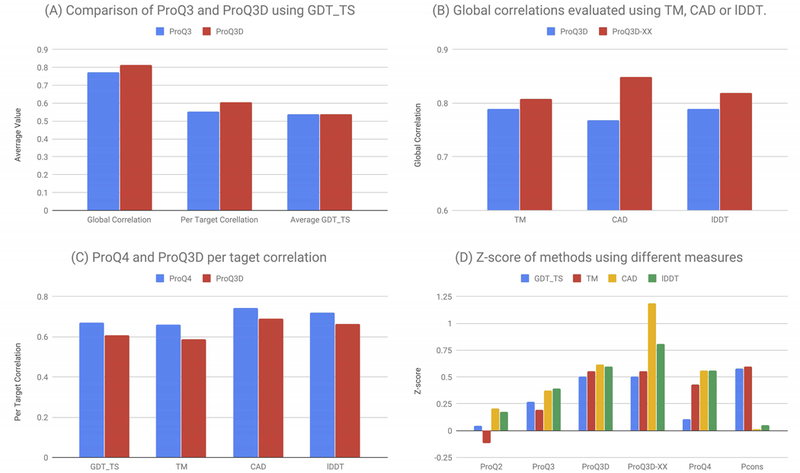
Here we compare the performance of different ProQ versions in CASP13. (A) Compares the difference in performance between ProQ3 and ProQ3D using GDT_TS as an evaluation criteria. Three measures are reported, global correlation, per target correlation and average GDT_TS score for the first ranked model. (B) Compares the performance of different versions of ProQ3D using the global correlation of all targets. Here evaluation is for different versions of ProQ3D trained on different target functions, with ProQ3D-XX is ProQ3 trained on the target function on which it is evaluated. ProQ3D is trained on S-score. (C) Compares ProQ3D and ProQ4 when it comes to per target correlation. (D) Plots the Z-score of performance for the different ProQ versions and Pcons for the global correlation.

Secondly, we examined the performance of different versions of ProQ3D trained to predict different model evaluations measures³⁷. Here, it can be seen that the version of ProQ3D trained on a specific target function performs better when evaluated on that target function, see Figure 6B.

It is well known that the full potential of EMA methods is not realized as for many targets the best available model is not ranked at position one. When developing ProQ4³⁸ one of the goals were to improve the ranking of targets. The better ranking is obtained by always presenting two models for the same target to the network and then train it to identify the better one. It can be seen in Figure 6C that ProQ4 is better at ranking than ProQ3D, so this goal was also achieved. However, as can be seen in Figure 6D the overall performance was not better for ProQ4 than for ProQ3D-XX (ProQ3D trained on the accuracy measure on which is evaluated).

Finally, it can be seen that all ProQ methods (as well as other single model methods) perform relatively better when evaluated on CAD and lDDT compared with consensus methods such as Pcons, see Figure 3 and 6D.

Han group - What did we learn

According to CASP13 assessment, SARTclust performed well both in selecting the best models and in the aspect of per-target correlation in global QA (Figure 2C). In particular, SARTclust performed best in all criteria of local QA such as ASE, MCC and correlation. Our clustering method is based on comparisons between the given model and the top-ranked models in the decoy set, which is slightly different from ModFOLDclust2^8,24 and Pcons⁸ based on all-against-all pairwise model comparisons. The better performance of SARTclust over ModFOLDclust2 and Pcons demonstrates the validity of the idea behind our clustering method. Further improvement in SARTclust would be accomplished by the progress of our single model accuracy estimation method, SART, through pre-selection step and weighting scheme.

The single model accuracy estimation method SART did not perform well in CASP13, although it contributes to the good performance of clustering method SARTclust through the step of selecting the reference set and weighting scheme. In our benchmarks on CASP11 prior to CASP13, it outperformed the well-known top single method ProQ2⁶ as shown in CASP13 abstract. However, it is outperformed by ProQ2 in this round. We plan to implement some directions to improve our single model method. First, more attention should be given to extracting of more valuable features such as prediction of residue-residue contact and residue-residue distance. Although SART incorporates residue-residue contact prediction, the performance of the in-house residue-residue contact prediction program is not good. So, it should be further upgraded in future. Besides, we will try to prepare the training data evenly, which is thought to be important for balanced prediction. Due to the bias in the composition of training data (medium- and low-quality models are more dominant than high-quality models in CASP9 data we used as training data), SART was ranked worse in the aspect of accuracy loss than in absolute accuracy estimation. It is expected that the performance improvement of the single model method SART will also make a good effect on the clustering method SARTclust.

McGuffin group - What did we learn

The ModFOLD7 server is continuously benchmarked in the Model accuracy Estimation (MAE) category using the CAMEO server¹⁰ (identified as server 28). The method has been independently verified to be an improvement on our previous methods (ModFOLD4 & ModFOLD6). At the time of writing, the ModFOLD7_(res)_lDDT method ranks among the top few QE servers on CAMEO.

Looking at global scoring evaluations on the CASP13 data, as expected the ModFOLD7_rank method was the best variant at ranking or selecting the best models and the ModFOLD7_cor variant was better at reflecting observed accuracy scores or estimating the absolute error, while he ModFOLD7 method was more balanced in terms of performance. For local scoring, the ModFOLD7_rank and ModFOLD7 variants performed better according to S-score and ModFOLD7_cor method according to lDDT.

Specific Improvements over ModFOLD6 from our in-house analysis using CASP11, CASP12 and CASP13 data were calculated for global and local scoring, and a summary of selected key results are shown in Figure 7. The ModFOLD7 variants showed small but significant improvements in both local scoring and selection of best models across all three datasets (CASP11–13), compared with the equivalent ModFOLD6 variants (Figure 7). The plots on left panels of Figure 7 show that ModFOLD7 rank outperforms ModFOLD6_rank in terms of selecting the best models measured by cumulative GDT_TS; a significant improvement on all 3 datasets. In the middle panels, the ModFOLD7_cor method outperforms ModFOLD6_cor in terms of the correlation of the global output score versus the GDT_TS score on some datasets. However no consistent improvement in global correlations was observed for ModFOLD7_cor over ModFOLD6_cor across all datasets, and any improvements seen were dependent on the chosen dataset and/or the observed score (e.g. ModFOLD7 outperforms ModFOLD6_cor according to the lDDT score on the CASP13 set, but not by GDT_TS). Finally, in terms of local accuracy estimates, based on both the lDDT scores (Figure 7, right panels) and S-scores, we also observed a significant improvement with the newer ModFOLD7 variants versus our older ModFOLD6 method.

Figure 7.

Histograms summarising the improvements in ModFOLD7 variants versus ModFOLD6 variants on CASP11–13 datasets. Model data from QA stages 1 and 2 are combined with duplicate models removed. Left panels show the ranking/model selection performance measures by cumulative GDT_TS scores of the top selected models by each method. Middle panels show Pearson correlation coefficients of global predicted accuracy versus observed accuracy according to GDT-TS. Right panels show performance of local accuracy estimates as measured by the Area Under the Curve (AUC) scores from ROC analysis using the lDDT observed local scores.

The consistent performance improvements of ModFOLD7 variants over ModFOLD6 were due to; 1. The addition of more input scores and correspondingly more input and hidden layer neurons to the neural network, 2. Training to different local target functions (the lDDT score as well as the S-score), and 3. Optimising for different evaluation metrics using a higher number of global scoring metrics.

Studer group - What did we learn

There is a tendency for harder modelling targets in CASP when compared to CAMEO. Low-resolution terms that primarily assess the likelihood of a correct overall fold (e.g. agreement terms/ backbone only statistical potentials), might have increased importance, compared to high-resolution terms that are mainly targeted at detecting local distortions in high-quality model structures (e.g. full atomic statistical potentials). We found that neural networks, if trained with appropriate data, are capable of adaptively weigh different terms to return accurate accuracy estimates for models of both origins, CASP and CAMEO (Table II).

FaeNNz has never been optimized to assess global model accuracy. However, given the nature of contact based scores such as lDDT or CAD, the average of accurate per-residue accuracy estimates can be expected to be a good approximation of the global accuracy. Especially in the case of lDDT, the score FaeNNz has been trained to predict, this assumption has been verified. According to the automated evaluation in CASP13, FaeNNz has the lowest average deviation between predicted score and actual global lDDT. This makes it the ideal tool to estimate the absolute global accuracy of a protein model and assess its suitability for the planned use case.

Venclovas group - What did we learn

Several observations regarding the VoroMQA performance in CASP13 can be made. Firstly, repacking side-chains prior to scoring with VoroMQA (done by VoroMQA-A) was not advantageous in any way. Thus, the performance of only the more straightforward server, VoroMQA-B, is discussed further. Also, for every VoroMQA-B score, the corresponding score by the previous VoroMQA version was calculated and recorded to assess if including hydrogen atoms affected the performance. For brevity, the older version is denoted onwards as VoroMQA(no H), and the newer one as VoroMQA(H).

The performance of VoroMQA in selecting best models is summarized in Figure 8A, which shows a histogram of the per-target selection losses. Here, the loss is defined as the difference between the z-scores of the model selected by VoroMQA and the actual best model for the target according to lDDT. Using other reference based scores instead of lDDT (e.g. GDT-TS, CAD-score) reveals similar tendencies. Figure 8A shows that the most substantial selection errors by VoroMQA(H) were made on those targets that correspond to the individual subunits pulled out of protein complexes. VoroMQA(H) performed significantly better (smaller losses) on the targets that are native monomers. VoroMQA(no H) showed similar selection performance. The reason why VoroMQA performs worse on targets that are not monomers in the native state can be easily explained. Structures of individual subunits withdrawn from protein complexes often exhibit energetically unfavorable solvent-accessible surface regions corresponding to protein-protein interaction interfaces. Such regions can be heavily penalized by VoroMQA, which works by estimating the energy but are not penalized by reference-based scores that only consider discrepancies in positions of corresponding atoms, not energy. Thus, to achieve the best selection results, it is more appropriate to use VoroMQA on structural models representing the native oligomeric state so that inter-chain interfaces can be assessed properly.

Figure 8:

(A) Histogram of VoroMQA losses in selecting best models. (B) Quantile-based grouping for global scores. (C) Quantile-based grouping for local scores (the box plots were drawn based on more than a million residue scores, outliers are not shown for clarity). Colored numbers under the horizontal axis are the empirical quantile values derived from the observed distributions of the different assessed scores.

The VoroMQA performance can also be assessed by asking how effectively the VoroMQA scores can group models according to their accuracy. Such grouping can be done using quantiles of distributions of VoroMQA scores. Figure 8B shows the results of the grouping analysis performed on the global scores of the models for the CASP13 targets that are native monomers (the results for all the CASP13 targets are similar, but with more outliers). Grouping was done using VoroMQA(no H), VoroMQA(H) and CAD-score. CAD-score was included for comparison to see how well a given reference-based score (CAD-score) can group models when judged by another reference-based score. In this case, the judge was lDDT, but the results were similar if the roles of lDDT and CAD-score were switched. Grouping was done using quantiles of 1/3 and 2/3 (33.3% and 66.7%) as thresholds. For every resulting group, the corresponding distribution of lDDT scores is depicted in Figure 8B via box plots. The box plots indicate that VoroMQA(no H) and VoroMQA(H) perform equivalently, although their corresponding quantile values are different. In general, the VoroMQA-based grouping is fairly similar to that based on CAD-score. This is quite remarkable considering that lDDT and CAD-score are some of the most similarly behaved and highly correlated reference-based scores⁵³.

The same analysis was also done for local (per-residue) scores. The results are shown in Figure 8C. The VoroMQA scores used in the analysis are raw VoroMQA local scores ranging from 0 to 1, not converted to distance deviations. Comparison of Figure 8C and Figure 8B reveals that the conclusions made for the grouping of global scores can also be applied to the grouping of local scores. One of the differences is that the grouping of local scores (at the level of residues) results in groups with more spread out corresponding distributions of lDDT scores (compared to the grouping according to the global scores). In addition, the group of residues with the lowest VoroMQA scores exhibit a tighter distribution of lDDT scores than the medium and high-scoring groups. In other words, poorly modeled regions are recognized more efficiently. Interestingly, CAD-score also shows a better agreement for residues in such regions.

Overall, based on the CASP13 results it can be concluded that the new enhancement (the addition of hydrogen atoms) neither improved nor impaired the VoroMQA performance. Thus, the VoroMQA version that does not use hydrogen atoms is more practical. It is faster and does not depend on additional tools for adding hydrogens. VoroMQA performs reasonably well in model selection, especially when evaluating structural models in the native monomeric or oligomeric state. Also, considering that VoroMQA is an unsupervised learning-based method that was not trained to predict any reference-based accuracy scores and does not use any additional data, it appears to be surprisingly robust in estimating both global and local accuracy.

Conclusions

We show that there has been a small but significant improvement since CASP12 in EMA methods. It can be noted that many of the improved methods use deep learning, but in different ways. The rapid development of deep learning models as exemplified here might indicate that the best way to use machine learning for model accuracy evaluations is still not developed. We also notice that on average the best EMA methods select models that are better than those provided by the best server. However, still, much more significant improvements could be achieved if there were possible ways to always select the best model for each target. Finally, we do notice systematic differences when using different model evaluations methods. Single model methods perform relatively better when using local evaluations methods.

References

- 1.Elofsson A et al. Methods for estimation of model accuracy in CASP12. Proteins 86 Suppl 1, 361–373 (2018). [DOI] [PubMed] [Google Scholar]
- 2.Roche DB, Buenavista MT & McGuffin LJ Assessing the quality of modelled 3D protein structures using the ModFOLD server. Methods Mol. Biol. 1137, 83–103 (2014). [DOI] [PubMed] [Google Scholar]
- 3.Wallner B & Elofsson A Can correct protein models be identified? Protein Sci. 12, 1073–1086 (2003). [DOI] [PMC free article] [PubMed] [Google Scholar]
- 4.Cao R, Bhattacharya D, Adhikari B, Li J & Cheng J Massive integration of diverse protein quality assessment methods to improve template based modeling in CASP11. Proteins 84 Suppl 1, 247–259 (2016). [DOI] [PMC free article] [PubMed] [Google Scholar]
- 5.Olechnovič K & Venclovas Č VoroMQA: Assessment of protein structure quality using interatomic contact areas. Proteins 85, 1131–1145 (2017). [DOI] [PubMed] [Google Scholar]
- 6.Ray A, Lindahl E & Wallner B Improved model quality assessment using ProQ2. BMC Bioinformatics 13, 224 (2012). [DOI] [PMC free article] [PubMed] [Google Scholar]
- 7.Sippl MJ Calculation of conformational ensembles from potentials of mean force. An approach to the knowledge-based prediction of local structures in globular proteins. J. Mol. Biol. 213, 859–883 (1990). [DOI] [PubMed] [Google Scholar]
- 8.Lundström J, Rychlewski L, Bujnicki J & Elofsson A Pcons: a neural-network-based consensus predictor that improves fold recognition. Protein Sci. 10, 2354–2362 (2001). [DOI] [PMC free article] [PubMed] [Google Scholar]
- 9.Ginalski K, Elofsson A, Fischer D & Rychlewski L 3D-Jury: a simple approach to improve protein structure predictions. Bioinformatics 19, 1015–1018 (2003). [DOI] [PubMed] [Google Scholar]
- 10.Zhang Y TM-align: a protein structure alignment algorithm based on the TM-score. Nucleic Acids Res. 33, 2302–2309 (2005). [DOI] [PMC free article] [PubMed] [Google Scholar]
- 11.Zemla AT Protein Classification Based on Analysis of Local Sequence-Structure Correspondence. (2006). doi: 10.2172/928169 [DOI] [Google Scholar]
- 12.Wallner B & Elofsson A Identification of correct regions in protein models using structural, alignment, and consensus information. Protein Sci. 15, 900–913 (2006). [DOI] [PMC free article] [PubMed] [Google Scholar]
- 13.Hou J, Wu T, Cao R & Cheng J Protein tertiary structure modeling driven by deep learning and contact distance prediction in CASP13. doi: 10.1101/552422 [DOI] [PMC free article] [PubMed] [Google Scholar]
- 14.Bower MJ, Cohen FE & Dunbrack RL Jr. Prediction of protein side-chain rotamers from a backbone-dependent rotamer library: a new homology modeling tool. J. Mol. Biol. 267, 1268–1282 (1997). [DOI] [PubMed] [Google Scholar]
- 15.Karasikov M, Pagès G & Grudinin S Smooth orientation-dependent scoring function for coarse-grained protein quality assessment. Bioinformatics (2018). doi: 10.1093/bioinformatics/bty1037 [DOI] [PubMed] [Google Scholar]
- 16.Lu M, Dousis AD & Ma J OPUS-PSP: an orientation-dependent statistical all-atom potential derived from side-chain packing. J. Mol. Biol. 376, 288–301 (2008). [DOI] [PMC free article] [PubMed] [Google Scholar]
- 17.Zhang J & Zhang Y A novel side-chain orientation dependent potential derived from random-walk reference state for protein fold selection and structure prediction. PLoS One 5, e15386 (2010). [DOI] [PMC free article] [PubMed] [Google Scholar]
- 18.Rykunov D & Fiser A Effects of amino acid composition, finite size of proteins, and sparse statistics on distance-dependent statistical pair potentials. Proteins 67, 559–568 (2007). [DOI] [PubMed] [Google Scholar]
- 19.Cao R, Bhattacharya D, Hou J & Cheng J DeepQA: improving the estimation of single protein model quality with deep belief networks. BMC Bioinformatics 17, 495 (2016). [DOI] [PMC free article] [PubMed] [Google Scholar]
- 20.Uziela K, Shu N, Wallner B & Elofsson A ProQ3: Improved model quality assessments using Rosetta energy terms. Sci. Rep. 6, 33509 (2016). [DOI] [PMC free article] [PubMed] [Google Scholar]
- 21.Shen M-Y & Sali A Statistical potential for assessment and prediction of protein structures. Protein Science 15, 2507–2524 (2006). [DOI] [PMC free article] [PubMed] [Google Scholar]
- 22.Olechnovič K & Venclovas Č Voronota: A fast and reliable tool for computing the vertices of the Voronoi diagram of atomic balls. J. Comput. Chem. 35, 672–681 (2014). [DOI] [PubMed] [Google Scholar]
- 23.Wang Z, Eickholt J & Cheng J APOLLO: a quality assessment service for single and multiple protein models. Bioinformatics 27, 1715–1716 (2011). [DOI] [PMC free article] [PubMed] [Google Scholar]
- 24.McGuffin LJ & Roche DB Rapid model quality assessment for protein structure predictions using the comparison of multiple models without structural alignments. Bioinformatics 26, 182–188 (2010). [DOI] [PubMed] [Google Scholar]
- 25.Adhikari B, Hou J & Cheng J DNCON2: improved protein contact prediction using two-level deep convolutional neural networks. Bioinformatics 34, 1466–1472 (2018). [DOI] [PMC free article] [PubMed] [Google Scholar]
- 26.Magnan CN & Baldi P SSpro/ACCpro 5: almost perfect prediction of protein secondary structure and relative solvent accessibility using profiles, machine learning and structural similarity. Bioinformatics 30, 2592–2597 (2014). [DOI] [PMC free article] [PubMed] [Google Scholar]
- 27.Kabsch W & Sander C Dictionary of protein secondary structure: Pattern recognition of hydrogen-bonded and geometrical features. Biopolymers 22, 2577–2637 (1983). [DOI] [PubMed] [Google Scholar]
- 28.Hou J, Cao R & Cheng J Deep convolutional neural networks for predicting the quality of single protein structural models. doi: 10.1101/590620 [DOI] [Google Scholar]
- 29.Wang Z, Tegge AN & Cheng J Evaluating the absolute quality of a single protein model using structural features and support vector machines. Proteins 75, 638–647 (2009). [DOI] [PubMed] [Google Scholar]
- 30.Cao R & Cheng J Protein single-model quality assessment by feature-based probability density functions. Scientific Reports 6, (2016). [DOI] [PMC free article] [PubMed] [Google Scholar]
- 31.Zhou H & Skolnick J GOAP: a generalized orientation-dependent, all-atom statistical potential for protein structure prediction. Biophys. J. 101, 2043–2052 (2011). [DOI] [PMC free article] [PubMed] [Google Scholar]
- 32.Wallner B & Elofsson A Quality Assessment of Protein Models. Prediction of Protein Structures, Functions, and Interactions 143–157 (2008). doi: 10.1002/9780470741894.ch6 [DOI] [Google Scholar]
- 33.Wallner B & Elofsson A Pcons5: combining consensus, structural evaluation and fold recognition scores. Bioinformatics 21, 4248–4254 (2005). [DOI] [PubMed] [Google Scholar]
- 34.Wallner B & Elofsson A Prediction of global and local model quality in CASP7 using Pcons and ProQ. Proteins: Structure, Function, and Bioinformatics 69, 184–193 (2007). [DOI] [PubMed] [Google Scholar]
- 35.Kim C & Cha G Concurrent Execution of Multiple Deep Learning Applications on GPU. in (2017). doi: 10.14257/astl.2017.148.07 [DOI] [Google Scholar]
- 36.Levitt M & Gerstein M A unified statistical framework for sequence comparison and structure comparison. Proc. Natl. Acad. Sci. U. S. A. 95, 5913–5920 (1998). [DOI] [PMC free article] [PubMed] [Google Scholar]
- 37.Uziela K, Menéndez Hurtado D, Shu N, Wallner B & Elofsson A Improved protein model quality assessments by changing the target function. Proteins 86, 654–663 (2018). [DOI] [PubMed] [Google Scholar]
- 38.Hurtado DM, Uziela K & Elofsson A Deep transfer learning in the assessment of the quality of protein models. (2018). [Google Scholar]
- 39.Cheng J, Randall AZ, Sweredoski MJ & Baldi P SCRATCH: a protein structure and structural feature prediction server. Nucleic Acids Research 33, W72–W76 (2005). [DOI] [PMC free article] [PubMed] [Google Scholar]
- 40.Zemla A LGA: A method for finding 3D similarities in protein structures. Nucleic Acids Res. 31, 3370–3374 (2003). [DOI] [PMC free article] [PubMed] [Google Scholar]
- 41.Cristobal S, Zemla A, Fischer D, Rychlewski L & Elofsson A A study of quality measures for protein threading models. BMC Bioinformatics 2, 5 (2001). [DOI] [PMC free article] [PubMed] [Google Scholar]
- 42.Zhang Y & Skolnick J Scoring function for automated assessment of protein structure template quality. Proteins 57, 702–710 (2004). [DOI] [PubMed] [Google Scholar]
- 43.McGuffin LJ et al. IntFOLD: an integrated web resource for high performance protein structure and function prediction. Nucleic Acids Res. (2019). doi: 10.1093/nar/gkz322 [DOI] [PMC free article] [PubMed] [Google Scholar]
- 44.Waterhouse A et al. SWISS-MODEL: homology modelling of protein structures and complexes. Nucleic Acids Res. 46, W296–W303 (2018). [DOI] [PMC free article] [PubMed] [Google Scholar]
- 45.Canutescu AA, Shelenkov AA & Dunbrack RL Jr. A graph-theory algorithm for rapid protein side-chain prediction. Protein Sci. 12, 2001–2014 (2003). [DOI] [PMC free article] [PubMed] [Google Scholar]
- 46.Jones DT Protein secondary structure prediction based on position-specific scoring matrices. J. Mol. Biol. 292, 195–202 (1999). [DOI] [PubMed] [Google Scholar]
- 47.Remmert M, Biegert A, Hauser A & Söding J HHblits: lightning-fast iterative protein sequence searching by HMM-HMM alignment. Nat. Methods 9, 173–175 (2011). [DOI] [PubMed] [Google Scholar]
- 48.Mariani V, Biasini M, Barbato A & Schwede T lDDT: a local superposition-free score for comparing protein structures and models using distance difference tests. Bioinformatics 29, 2722–2728 (2013). [DOI] [PMC free article] [PubMed] [Google Scholar]
- 49.Studer G, Biasini M & Schwede T Assessing the local structural quality of transmembrane protein models using statistical potentials (QMEANBrane). Bioinformatics 30, i505–11 (2014). [DOI] [PMC free article] [PubMed] [Google Scholar]
- 50.Haas J et al. Continuous Automated Model EvaluatiOn (CAMEO) complementing the critical assessment of structure prediction in CASP12. Proteins 86 Suppl 1, 387–398 (2018). [DOI] [PMC free article] [PubMed] [Google Scholar]
- 51.Word JM, Lovell SC, Richardson JS & Richardson DC Asparagine and glutamine: using hydrogen atom contacts in the choice of side-chain amide orientation. J. Mol. Biol. 285, 1735–1747 (1999). [DOI] [PubMed] [Google Scholar]
- 52.Uziela K, Menéndez Hurtado D, Shu N, Wallner B & Elofsson A ProQ3D: improved model quality assessments using deep learning. Bioinformatics 33, 1578–1580 (2017). [DOI] [PubMed] [Google Scholar]
- 53.Olechnovič K, Monastyrskyy B, Kryshtafovych A & Venclovas Č Comparative analysis of methods for evaluation of protein models against native structures. Bioinformatics 35, 937–944 (2019). [DOI] [PMC free article] [PubMed] [Google Scholar]