Identifying loci with breeding potential across temperate and tropical adaptation via EigenGWAS and EnvGWAS

Abstract

Understanding the genomic basis of adaptation in maize is important for gene discovery and the improvement of breeding germplasm, but much remains a mystery in spite of significant population genetics and archaeological research. Identifying the signals underpinning adaptation are challenging as adaptation often coincided with genetic drift, and the base genomic diversity of the species in massive. In this study, tGBS technology was used to genotype 1,143 diverse maize accessions including landraces collected from 20 countries and elite breeding lines of tropical lowland, highland, subtropical/midaltitude and temperate ecological zones. Based on 355,442 high‐quality single nucleotide polymorphisms, 13 genomic regions were detected as being under selection using the bottom‐up searching strategy, EigenGWAS. Of the 13 selection regions, 10 were first reported, two were associated with environmental parameters via EnvGWAS, and 146 genes were enriched. Combining large‐scale genomic and ecological data in this diverse maize panel, our study supports a polygenic adaptation model of maize and offers a framework to enhance our understanding of both the mechanistic basis and the evolutionary consequences of maize domestication and adaptation. The regions identified here are promising candidates for further, targeted exploration to identify beneficial alleles and haplotypes for deployment in maize breeding.

1. INTRODUCTION

When a species migrates from one ecosystem to another, changes in various factors, such as climate and geographical surroundings, will result in adaptive changes of the allelic composition of the population. In evolutionary biology and ecology, it is important to identify loci under selection or adaption (Field et al., 2016; Stephan, 2016). In conventional analysis, identifying adaption‐ or evolution‐related loci is conducted via a variety of analytical methods, such as the F _ST scan (Wright, 1951), integrated haplotype score (iHS) (Voight, Kudaravalli, Wen, & Pritchard, 2006), composite of multiple signals (CMS) (Grossman et al., 2010), cross‐population extended haplotype homozygosity (XP‐EHH) (Sabeti et al., 2007), a multiple‐locus composite likelihood ratio (XP‐CLR) and singleton density score (SDS) (Field et al., 2016). Among these, the F _ST method that has been widely applied in plants relies on a prior sampling scheme or knowledge of the subpopulation, often unknown or hard to define, or on haplotype‐based inference (Field et al., 2016).

Recently, Chen, Lee, Zhu, Benyamin, and Robinson (2016) proposed a single‐marker regression approach based on principal component analysis (or eigen‐analysis), called EigenGWAS. Conceptually similar to genome‐wide association studies (GWAS), the analysis procedure of EigenGWAS is similar to the conventional regression analysis for GWAS but the phenotype is substituted by an eigenvector capturing genetic variation of the studied population. The regression coefficient of EigenGWAS approximates that of F _ST. In recent studies, EigenGWAS has been successfully used to identify selection signals in species such as human (Parolo, Lacroix, Kaput, & Scott‐Boyer, 2017) and in wild birds (Bosse et al.., 2017; Kim et al., 2017). These studies identified the genes under selection or adaption and illustrated how genetic signatures of selection translate into variation in phenotype fitness.

Previous studies have identified a number of maize genes under selection during domestication (Table S1), for example: teosinte branched1 (tb1), which modifies plant architecture and significantly reduces the development of tillers (Wang, Stec, Hey, Lukens, & Doebley, 1999); c1 governing the tissue‐specific expression of anthocyanin biosynthesis (Hanson et al., 1996); bt2, ae1 and su1, which encode components of the starch biosynthetic pathway (Whitt, Wilson, Tenaillon, Gaut, & Buckler, 2002); zagl1, a putative transcription factor (Vigouroux et al., 2002); d8 and ts2 involved in plant height, flowering time and sex determination, and exhibiting a selection imprint in teosintes (Harberd & Freeling, 1989; Irish & Nelson, 1993; Thornsberry et al., 2001); and y1, which encodes phytoene synthase and that has undergone recent selection for endosperm colour (Palaisa, Morgante, Tingey, & Rafalski, 2004). Teosinte glume architecture1 (tga1), a member of the SBP‐box gene family of transcriptional regulators, has been identified as conferring naked kernels (Wang, Studer, Zhao, Meeley, & Doebley, 2015), and grassy tillers1 (gt1), which encodes a homeodomain leucine zipper transcription factor, experienced a tissue‐specific gain in expression in maize that is associated with suppressing the initiation of multiple ears per plant such that only one or two large ears are formed (Whipple et al., 2011; Wills et al., 2013). In addition, Hufford et al. (2012) identified 484 chromosomal regions associated with domestication from wild teosintes to maize landraces and another 695 chromosomal regions associated with crop improvement from a set of 75 teosintes and maize lines. Tian, Stevens, and Buckler (2009), using 28 diverse maize inbred lines and 16 teosintes, discovered a large region on chromosome 10 involved in adaptation or domestication that has been the target of strong selection during maize domestication. More recently, Gage, White, Edwards, Kaeppler, and de Leon (2018) identified that selection impacted maize male inflorescence morphology through a comparison of 41 unselected early generation maize stiff stalk lines and 21 highly selected elite ex‐PVP lines.

Environmental GWAS (EnvGWAS) represents the associations between single nucleotide polymorphism (SNP) alleles and the original environment of accessions. Application of this approach can uncover the genetic basis of environmental adaption (Jones et al., 2012; Lasky et al., 2015; Turner, Bourne, Von Wettberg, Hu, & Nuzhdin, 2010). To help breed climate‐adapted varieties, researchers explored the impact of environment on domestication and found evidence of rapid evolution in response to environmental change (Bosse et al., 2017; Gaut, Seymour, Liu, & Zhou, 2018; Lasky et al., 2015). By de novo sequencing the maize EDMX‐2233 genotype of the Palomero Toluqueño (Palomero) landrace, a highland popcorn from San Lorenzo Teotuitlán, Mexico, Vielle‐Calzada et al. (2009) found that environmental factors related to the metal content of local soils may have been important in maize domestication. Navarro et al. (2017) found that 61.4% of the SNPs associated with flowering time were associated with altitude in a study of 4,471 maize landraces. These insights provide empirical support that genomic determinants of environmental adaptation can be identified, and this area merits further study.

Here, we used genomic characterization of 1,143 maize accessions from 20 countries, conducting EigenGWAS to identify genomic regions associated with local adaptation, and EnvGWAS to identify genomic regions associated with high‐resolution, long‐term geographical information system (GIS) data in the collection sites. The selection regions uncovered by this diverse panel enrich our understanding of the influence of environmental change on adaptation in maize, and can be used to facilitate the development of new elite cultivars adapted to changing environmental conditions in the face of climate change, a serious threat to global food security, sustainable development and poverty eradication.

2. MATERIALS AND METHODS

2.1. Plant materials

In this study, a total of 1,143 maize accessions were collected from 20 countries (Figure 1), including 11 teosinte inbred lines, 764 landraces sampled from the maize collection of the CIMMYT germplasm bank (MGB), 290 CIMMYT elite maize lines (CMLs) and 78 popcorn lines from the USDA Ames inbred collection (Romay et al., 2013). The 11 teosinte inbred lines were developed from wild teosinte materials under the Teosinte Inbred Project, 10 of which belong to subspecies parviglumis and one (ISU_TIL25) belongs to the subspecies mexicana. The teosinte information can be found in GRAMENE (http://archive.gramene.org/db/diversity/diversity_view?search_for=TIL%26object=div_passport%252Cdiv_synonym%26db_name=diversity_maize%26x=0%26y=0%26action=list). The 764 maize landraces selected originated from 20 countries representing broad adaptation and, compared with elite lines, broader genomic diversity. A panel of 290 CMLs was chosen from the complete CML set, comprising 573 lines at the time of the study. Selection of the CMLs was performed considering representation of the three major environmental adaptation groups (Lowland Tropical, Subtropical/Midaltitude and Highland Tropical subgroups), the described pedigrees (https://data.cimmyt.org/dataset.xhtml?persistentId=hdl:11529/10246) and known genomic relationships between the lines (Wu et al., 2016) in order to maximize the diversity captured by the 290 entry set. Passport information of the 764 maize landraces and the 290 CMLs can be found at http://hdl.handle.net/11529/10548183. The 78 popcorn inbred lines were obtained from the USDA‐ARS North Central Regional Plant Introduction Station (NCRPIS) in Ames, Iowa (Romay et al., 2013). Line identifiers can be found at http://hdl.handle.net/11529/10548183 and associated passport information is available from the U.S. National Plant Germplasm System at https://npgsweb.ars-grin.gov/gringlobal/search.aspx.

Figure 1.

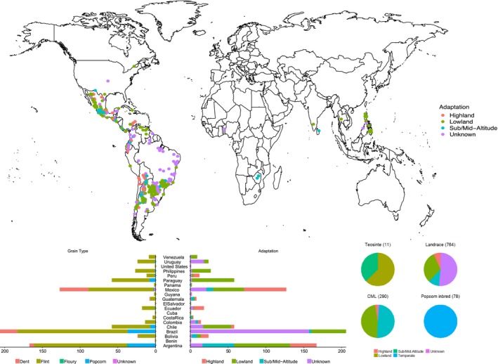
The geographical and adaptive distribution of the 1,143 maize collection. Lines cannot be assigned a geolocation origin so are not displayed on the map [Colour figure can be viewed at http://wileyonlinelibrary.com]

Of the 1,143 maize germplasm, 764 were open pollinated landraces and 379 were inbred lines. A summary of the descriptors for this panel of 1,143 accessions is available in Table S2. The maize materials in this study represent diverse ecological adaptation including tropical lowland, highland, subtropical/midaltitude and temperate, covering major ecotypes of maize resources developed during domestication and breeding.

2.2. Plant sampling and SNP genotyping

The germplasm panel was genotyped using genotyping‐by‐sequencing (tGBS) technology (Data2Bio LLC), an approach which simplifies the preparation of high‐quality GBS sequencing libraries and promises higher SNP calling accuracy (Ott et al., 2017). Compared with conventional genotyping‐by‐sequencing (cGBS) (Elshire et al., 2011), tGBS is more accurate in genotyping heterozygous sites and is therefore more relevant when exploring heterogeneous and heterozygous landrace populations. For each landrace, DNA was extracted from bulked leaf tissue obtained from ~12 selfed progeny of a single plant. In contrast, for each inbred line DNA was extracted from a single plant.

To identify polymorphic sites for each maize accession, alleles which differ from the reference genome (https://www.maizegdb.org/genome/genome_assembly/B73%2520RefGen_v3) were scanned. Excluding the first and last 3 bp of each read, only sites with PHRED quality ≥20 represented by at least five reads were retained. Only bi‐allelic sites with overall allele frequency ≥80% were considered to be polymorphic. Homozygous genotype sites were defined as five or more reads of major allele and overall major allele reads accounting for ≥90%; while heterozygous genotype sites were defined with two or more reads for each of two alleles, each accounting for at least 20% of the total reads. Sites not matching these criteria were assigned as missing.

Genotype calls were further filtered to improve quality via the following steps: (1) SNPs that had a minor allele frequency (MAF) of ≥1%, heterozygosity rate ≤0.2 + 2p(1 − p), where p is the MAF, and missing data rate ≤50% were retained; and (2) samples with missing data rate ≥90% were removed. There were two sources of missing information in the data set: one was missing genotypes for the covered sites by tGBS due to the limited read coverage for some maize accessions; the other was uncovered sites due to the reduced representation of the genome using tGBS technology. Therefore, imputation in this study was conducted for both sources (i.e., filling the missing genotypes and deducing the uncovered sites). The filtered genotypes retained through Steps (1) and (2) were imputed by the following steps. (3) Regarding imputation of the missing genotypes for the tGBS data set, beagle version 4.1 (Browning & Browning, 2016, 2007) with default parameters (i.e., window = 50,000, overlap = 3,000; niterations = 15, and cluster = 0.005) without reference panel was used (this is the most suitable approach for landrace germplasm, Swarts et al., 2014). (4) For imputation of the uncovered sites to increase marker density with high statistical accuracy, the genetic variation on HapMap version 3.2.1 was used as the reference panel, which consists of 1,210 maize lines, includes 83 million SNPs (the 30 million "LLD" SNPs are high‐confidence markers) and covers global predomesticated and domesticated Zea mays varieties (available from the Panzea website: http://cbsusrv04.tc.cornell.edu/users/panzea/filegateway.aspx?category=Genotypes). To control the quality of this reference panel, it was filtered to 7,593,114 SNPs that met the criteria MAF ≥5%, minimum calling rate ≥30% and sample missing rate ≤50% on each chromosome (Table S3). The SNPs retained from Step (3) were further imputed using beagle version 4.1 with the filtered reference panel and default parameters.

2.3. Population structure analysis

For pairwise taxa, distance matrices using the p‐distances model were calculated by the tassel version 5.2 software (Glaubitz et al., 2014). Neighbour‐joining (NJ) trees were constructed with 1,000 bootstraps using the tassel version 5.2 software and were visualized using the online tool itol version 4 (Letunic & Bork, 2016). Principal component analysis (PCA) was conducted using plink 1.9 (https://www.cog-genomics.org/plink2; Chang et al., 2015) for individuals in the HapMap3 reference population and the 1,143 maize materials used in this study.

2.4. Selection analysis

Identification of loci under selection through GWAS of eigenvectors was implemented using EigenGWAS (Chen et al., 2016). Using high‐quality SNPs to generate a genetic relationship matrix, the top 10 eigenvalues and their corresponding eigenvectors were calculated. SNP effects, nearly equivalent to F _ST, could be estimated by regressing each SNP for a selected eigenvector. In principle, the estimated genetic effect for each locus is driven by genetic drift which is random, and/or selection which is directional. To filter out the genetic drift component, we adjusted the p‐value with a genomic control factor (Devlin & Roeder, 1999), and consequently the corrected p‐value, P _GC, was used for detecting the loci under selection. To determine the cutoff of significance of loci under direct selection, the first eigenvector was reshuffled 1,000 times to evaluate the null distribution. The 95th quantile of the 1,000 most significant p‐values across 1,000 permutations was used as the significance threshold. After log₁₀ transformation, a p‐value threshold of 5.87 for an experiment‐wise type I error rate of 0.05 was used for the EigenGWAS analyses for each of the 10 eigenvectors.

2.5. GIS data extraction and EnvGWAS

Climate data were extracted from extrapolated climate grids (Fick & Hijmans, 2017) at 30 s (~1 km) resolution for 509 maize landrace populations. Raw data files for monthly long‐term average (1970–2000) minimum (tmin), maximum (tmax), averaged temperature (tavg), rainfall (prec), vapour pressure (vapr) and solar radiation (srad) were downloaded from http://worldclim.org/version2 as well as soil pH (ph5) at 5 cm depth (Hengl et al., 2017) from https://soilgrids.org and converted to ESRI grid format for storage and extraction. Curated georeferenced collection site locations were used to extract climate and soil pH values for accessions using the spatial analyst toolbox in ESRI arcmap 10.6. Genome‐wide association was performed using a general linear model (GLM; Price et al., 2006) implemented by a memory‐efficient, visualization‐enhanced and parallel‐accelerated tool for GWAS (MVP; https://github.com/XiaoleiLiuBio/MVP/) with seven GIS data parameters (tmax, tmin, tavg, srad, vapr, ph5, and prec) as response variables. The p‐value threshold was determined using permutation tests by 1,000 times reshuffling of the of tmin trait. As a result, the SNPs with a log p‐value greater than 5.77 were considered to be statistically significant for a type I error rate of 0.05.

2.6. Linkage disequilibrium and haplotype analysis

The squared correlation of allele frequency (r ²) was calculated by plink 1.9 (https://www.cog-genomics.org/plink2; Chang et al., 2015) to evaluate linkage disequilibrium (LD) in the maize panel. Pairwise r ² values were plotted against genomic distance in a 1‐kb window, and a locally weighted polynomial regression (LOESS) curve was fitted using r software. An EHH test was conducted for each of the selected SNPs within the 2‐Mb region, identifying long and frequent haplotypes as implemented in the R package rehh (Gautier & Vitalis, 2012). The same package was used for the bifurcation diagrams of alleles. We also screened for population‐specific extended haplotypes with Rsb, a statistic that compares EHH between populations to detect between‐population selection. The haplotype data were also presented as bifurcation diagrams to clearly illustrate the breakdown/maintenance of haplotype structure.

2.7. Gene annotation and enrichment analysis

Functional annotations of the target SNPs were performed using snpeff (Cingolani et al., 2012). The Maize B73 reference V3 gene annotation as a gff3 file type was downloaded from the Maize Genetics and Genomics Database (MaizeGDB) (https://www.maizegdb.org/assembly). Functional enrichment analysis of the annotated genes was performed via the ClueGO plug‐in for cytoscape (Bindea et al., 2009).

2.8. GWAS analysis on popping trait

To map the popping‐related loci and test if they had undergone selection, the 1,143 maize accessions were classified into two groups: (1) a popping group with 264 landrace populations and the 78 popcorn inbred lines, and (2) a nonpopping group with 500 landrace populations and the 290 CMLs. The artificial phenotypes of Group (1) were all set as 1, while those of Group (2) were all set as 0. With the phenotypes so defined, GWAS was performed based on a GLM using mvp software (https://github.com/XiaoleiLiuBio/MVP/). The first five principal components calculated by plink 1.9 (https://www.cog-genomics.org/plink2; Chang et al., 2015) were included as population structure. The same whole‐genome p‐value cutoff as that used in EnvGWAS (i.e., 2.03E‐06) was used to declare the significant SNPs associated with the trait of popping.

3. RESULTS

3.1. tGBS genotypes

In total, 0.31 terabases (Tb) of sequence data from 2.5 billion quality‐trimmed reads were generated from the 1,145 maize accessions via tGBS (Ott et al., 2017) (Figures S1 and S2). After alignment to the reference genome (B73 Zea mays AGPv3 genome, http://cbsusrv04.tc.cornell.edu/users/panzea/download.aspx?filegroupxml:id=29), 3,713,115 SNPs were identified. Two accessions with missing rates >90% were removed (i.e., one popcorn line AMES_28995 and one elite line CML131). Of the 3,713,115 tGBS SNPs, 65,540 were retained after filtering for MAF and heterozygosity (Figure S3). The 65,540 tGBS SNPs were imputed without a reference panel. To further capture the genetic variation across the maize genome, the tGBS 65,540 SNPs were also imputed to 359,618 high‐quality SNPs using maize HapMap V3 as a reference panel (Figure 2a and Tables S3 and S4). Finally, the union of the two SNP sets (N = 414,124 SNPs; Figure 2a) was filtered by MAF and heterozygosity under the same criteria as mentioned above, resulting in 355,442 high‐quality SNPs, which were retained for further analysis. This SNP set has an average MAF of 0.241 and an average heterozygosity of 0.133 (Figure 2b,c). The heterozygosity rates of over 85% of the accessions were lower than 20% (Figure 2c,d), which is comparable with those from GBS 4K landraces (average = 4.2%) by Navarro et al. (2017).

Figure 2.

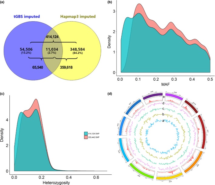
The intersection of SNPs for the data set imputed by tGBS and imputed by HapMap3 (a), the frequency of minor alleles (b) and heterozygosity (c) of 1,143 maize accessions based on the 414,124 SNP data set before filtering and the 355,442 SNP data set after filtering, SNPs identified in the 1,143 accessions (d): “a” to “d” depict the nucleotide divergence polymorphism (π) on population “Popcorn inbred” (blue), “CMLs” (dark yellow), “Landrace” (green), and “Teosinte” (purple), respectively, and “e” presents 355,442 SNP density [Colour figure can be viewed at http://wileyonlinelibrary.com]

3.2. Genetic diversity within the 1,143 accessions

In general, the results from phylogenetic analyses and PCA were consistent (Figure 3 and Figure S4). The NJ tree revealed clear differentiation of the 1,143 accessions into four major groups: teosintes, landraces, CMLs and popcorn inbred. There were some intersections between CMLs and landraces and some between popcorn inbred and landraces (Figure 3). Results from the PCA showed that the genetic diversity of 1,143 accessions used in this study covered most of the genetic diversity of HapMap 3, reflecting the enormous genetic diversity in maize. Two groups of CMLs and landraces clustered together, while popcorn inbred lines were scattered among the landraces (Figure S4).

Figure 3.

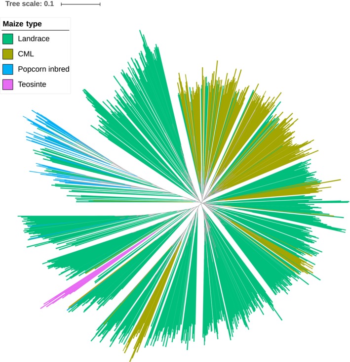
Neighbour‐joining tree based on the 1,143 maize panel and computed on a simple matching distance matrix for the filtered SNPs [Colour figure can be viewed at http://wileyonlinelibrary.com]

The first five eigenvectors were compared pair‐wise based on maize type and adaptation (Figure 4). Interestingly, most of Ev1 for CMLs were negative, but were positive for teosintes and popcorn inbred. Ev1 for landraces were approximately half positive and half negative. With regard to maize type (landrace, CML, temperate popcorn lines, teosinte lines), the popcorn inbred group could be clustered separately from other groups by plotting Ev1 versus Ev2, Ev2 versus Ev3, Ev2 versus Ev4, and Ev2 versus Ev5, suggesting that Ev2 may be reflecting the temperate versus tropical adaptation. In terms of the Ev distribution for adaptation, the proportion of negative and positive values varied across Ev1–Ev5 for lowland, sub/midaltitude, and highland (Figure 4).

Figure 4.

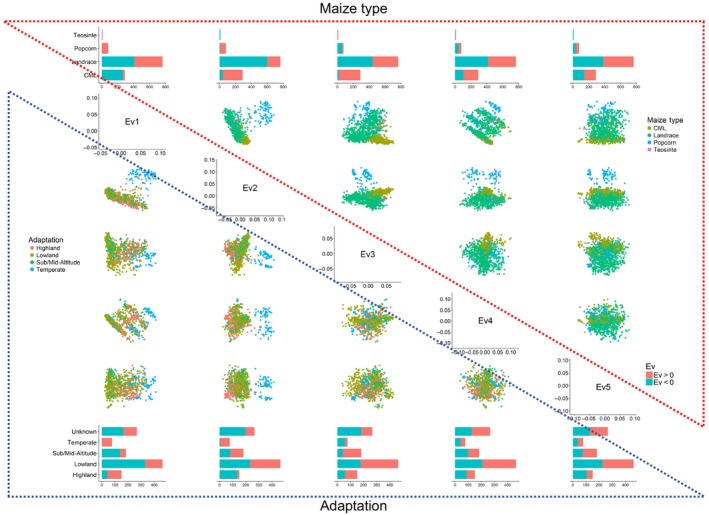
PCA plots of five eigenvectors (Ev1–Ev5) of different maize types and adaptation groups for the 1,143 maize panel [Colour figure can be viewed at http://wileyonlinelibrary.com]

There was high LD for most of the pairwise comparisons when using the 355,442 SNP loci, primarily because the imputation procedure was based on the LD block inferred from the reference data set, which therefore lowered the rate of LD decay. Therefore, the unimputed 65,540 SNP data set was used to conduct the LD analyses. The extent of LD decay (r ² = .1) was found at an intermarker genetic distance of 2.5 kb (Figure S5).

3.3. Adaptation model of maize using the 1,143 maize accessions

EigenGWAS analyses were conducted using the entire data set for the first 10 eigenvectors. Mean genetic relatedness across the maize collection was −0.0014, indicating that the effective sample number of the panel was 712.44, and the effective number of genome segments was 34.65. The largest eigenvalue was 143.45, explaining about 12.6% of the total genetic variation; the 10th largest eigenvalue was 17.14, explaining about 1.5% of the total genetic variation; the top 10 eigenvalues represented ~40.5% of the overall genetic variation (Table 1), indicating that the complicated population structure of maize could not be captured by the largest eigenvalue only. In comparison, a simple population structure such as the genetic structure of northwestern and southern European humans could be largely explained by the largest eigenvalue alone (Chen et al., 2016; Novembre et al., 2008). For a diverse population such as Human HapMap, which covers multi‐ethnicities, the largest eigenvalue explained about 10% of the total genetic variation, and left more variation to be captured by other eigenvalues (table 1 in Chen et al., 2016). The genomic inflation factor that is commonly used in adjusting population stratification for GWAS (Devlin & Roeder, 1999), namely λ_GC calculated from EigenGWAS, ranged from 82.38 to 4.16 (Table 1 and Figure S6). After correction by λ_GC, the SNPs with −log₁₀(P _GC) exceeding the threshold of 5.87 were declared as the loci under selection at the genome‐wide level. Upon positive or negative coordinates on the corresponding eigenvector, two subgroups were implicitly defined for all accessions, and their selection differentiation was quantified by EigenGWAS via the 1df chi‐square test statistics, which was proportional to F _ST.

Table 1.

Summary statistics from EigenGWAS for 1,143 maize collections

Eigenvector (Ev)	Eigenvalue	Mean F ST	GWAS λGC	Number of GWAS hits
1	143.454	0.096	82.383	20
2	83.941	0.048	47.830	105
3	53.03	0.034	27.793	1
4	40.445	0.022	11.213	14,362
5	31.611	0.019	4.156	22,125
6	29.246	0.017	12.276	6,310
7	26.034	0.017	6.229	5,707
8	20.785	0.012	7.720	4,965
9	17.511	0.010	6.004	4,044
10	17.143	0.010	8.138	0

λ_GC is defined as the ratio between the 1df χ ² value of the median p‐value of .455 minus the 1df χ ² value of the p‐value of .5.

To facilitate the comparison, scanning results from −log₁₀(P _GC) and F _ST are shown together as a Miami plot (Figure 5). The peaks from −log10(P _GC) and F _ST nearly mirrored each other, indicating reasonable grouping as defined by EigenGWAS. In total, 57,639 significant SNPs were identified in the 10 EigenGWAS analyses (Table 1, Figure 5 and Table S5), with no significant SNPs obtained using Ev10, and the most hits (i.e., 22,125 SNPs) using Ev5. The distribution of the identified SNPs across different chromosomes varied considerably, with chromosome 3 (i.e., 14,382 SNPs) having the highest numbers of SNPs and chromosomes 6 and 7 (i.e., one SNP each) the lowest. Thirteen selection regions were determined via an LD block size of 0.5 Mb from 57,639 significant SNPs, with two regions on each of chromosomes 1 and 3, three regions on chromosomes 2, and one region on each of chromosomes 4, 5, 6, 7, 8 and 10 (Table 2). The most significant region was detected on chromosome 2 with P _GC reaching 8.65e‐37 by three eigenvectors (i.e., Ev5, Ev7 and Ev8) in EigenGWAS. Twenty‐eight genes were annotated in this particular region.

Figure 5.

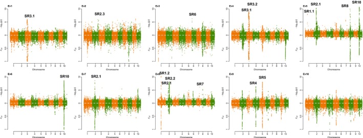
Miami plot from EigenGWAS (upper for P _GC and lower for F _ST) for Ev1–Ev10 based on the 1,143 maize panel. P _GC is the p‐values corrected by λ_GC in EigenGWAS. Ev1–Ev10 are the first 10 eigenvectors, each of which was used as phenotype for the single‐marker association study based on nearly 355,442 markers in EigenGWAS [Colour figure can be viewed at http://wileyonlinelibrary.com]

Table 2.

Thirteen regions under selection identified in the 1,143 maize panel using EigenGWAS

Region	Start	End	Distance	Ev	p	P GC	F ST	Annotation	Gene number	Gene description	Reported
SR1.1	S1_79266034	S1_79266082	48	Ev5	1.28E−31	9.82E−09	0.0609	intergenic_region	0	GRMZM2G048821‐GRMZM2G456401	Beissinger et al. (2014)
SR1.2	S1_122588015	S1_124631827	2,043,812	Ev8	3.34E−96	6.97E−14	0.4327	missense_variant, 3_prime_UTR_variant, 5_prime_UTR_variant, splice_region_variant&intron_variant	5	glucan endo−1,3‐beta‐glucosidase 7, disease resistance response protein 206	Beissinger et al. (2014)
SR2.1	S2_90633341	S2_97732843	7,099,502	Ev5, Ev7, Ev8	3.43E−219	8.65E−37	0.2687	stop_retained_variant, 3_prime_UTR_variant, 5_prime_UTR_variant, 5_prime_UTR_premature_start_codon_gain_variant, missense_variant, splice_region_variant&synonymous_variant	28	hypothetical protein LOC100272669
SR2.2	S2_113040712	S2_122223253	9,182,541	Ev8	3.46E−59	5.34E−09	0.1782	3_prime_UTR_variant, 5_prime_UTR_variant, missense_variant	18	legume lectins beta domain containing protein
SR2.3	S2_200735084	S2_200738759	3,675	Ev2	4.19E−249	1.10E−06	0.171	3_prime_UTR_variant	1	cytokinin‐O‐glucosyltransferase 2
SR3.1	S3_73092472	S3_85086886	11,994,414	Ev1, Ev4	0	1.12E−09	0.886	3_prime_UTR_variant, 5_prime_UTR_variant, missense_variant, start_lost, missense_variant&splice_region_variant, splice_region_variant&intron_variant, splice_region_variant&synonymous_variant	20	glycosyltransferase family 28 C‐terminal domain containing protein
SR3.2	S3_100100348	S3_106656690	6,556,342	Ev4	6.56E−103	1.27E−10	0.2026	missense_variant, 3_prime_UTR_variant	9	hypothetical protein LOC100217119
SR4	S4_110464865	S4_110904488	439,623	Ev9	4.35E−35	4.65E−07	0.1359	missense_variant, 5_prime_UTR_variant	1	hypothetical protein LOC100280215
SR5	S5_103048851	S5_109807152	6,758,301	Ev9	2.07E−45	8.00E−09	0.1455	missense_variant, start_lost, 3_prime_UTR_variant	6	hypothetical protein LOC100277634	Vielle‐Calzada et al. (2009)
SR6	S6_14879186			Ev3	2.47E−155	4.77E−07	0.2329	intergenic_region	0	GRMZM5G884722‐AC186406.4_FG006
SR7	S7_115180718			Ev8	2.53E−43	6.91E−07	0.1211	intergenic_region	0	GRMZM2G071059‐GRMZM2G171408
SR8	S8_41930480	S8_55983961	14,053,481	Ev5	8.69E−115	5.25E−29	0.3741	3_prime_UTR_variant, missense_variant, 5_prime_UTR_variant, splice_region_variant&intron_variant	35	Poly [ADP‐ribose] polymerase 2, SUMO protease, rapid alkalinization factor 1, ATP‐dependent Clp protease proteolytic subunit 1
SR10	S10_37844852	S10_46876871	9,032,019	Ev5, Ev6	2.62E−107	3.40E−27	0.4204	missense_variant&splice_region_variant, stop_gained, missense_variant, 5_prime_UTR_variant, 5_prime_UTR_premature_start_codon_gain_variant, stop_lost, splice_region_variant, splice_region_variant&intron_variant	21	UDP‐galactose translocator, retrotransposon protein SINE subclass

Of the 13 selection regions, three (i.e., SR2.1, SR3.1 and SR10) were repeatedly detected by more than one eigenvector, and three regions (i.e., SR1.1, SR1.2 and SR5) were reported in previous studies (Table 2). Region SR1.1 with a length of 48 bp and SR1.2 with a length of 2 Mb were identified as highly divergent with a soft‐sweep model (Beissinger et al., 2014). Genes encoding glucanendo‐1,3‐beta‐glucosidase 7 and disease resistance response protein 206 were located in the region of SR1.2. Region SR5 with a length of 6.75 Mb had been reported as SMS18, encoding a P‐type copper translocator that also detoxifies heavy metals from the Palomero Genome (Vielle‐Calzada et al., 2009). Ten selection regions were first reported in this study, and only a fraction of the newly identified candidate genes have been functionally characterized: for example, legume lectins beta domain containing protein in SR2.2, cytokinin‐O‐glucosyltransferase 2 in SR2.3, glycosyltransferase family 28 C‐terminal domain containing protein in SR3.1, poly [ADP‐ribose] polymerase 2, SUMO protease, rapid alkalinization factor 1 and ATP‐dependent Clp protease proteolytic subunit 1 in SR8, and UDP‐galactose translocator and retrotransposon protein SINE subclass in SR10 (Table 2).

To further validate the 13 selection regions, six SNPs (i.e., S2_95391165, S5_107377632, S10_40760398, S10_40760575, S10_40949675 and S10_40949963, Figures S7–S12), associated with more than one eigenvector contained within genes with annotations such as “start_lost,” “stop_gained,” “stop_lost” and “stop_retained_variant” functions (Table S6), were chosen for further analysis because they would be the most likely to alter known gene function.

S2_95391165 (P _GC = 8.65e‐37 under Ev7 and P _GC = 5.17e‐09 under Ev5; Table S5), located within SR2.1, was a stop‐retained variant in gene GRMZM2G101250, where patterns of genetic variation revealed a clear signature of recent selection (Figure S7). EHH tests also showed that the S2_95391165‐G haplotypes extended further than the reference S2_95391165‐A haplotypes (Figure S13). Large differences in bifurcation diagrams of S2_95391165‐G haplotypes and S2_95391165‐A haplotypes could be observed across the four maize types (Figure S7). For SNP S2_95391165, the averaged Ev1 values for each genotype were significantly different (p < 2.2e‐16), and the frequency of each genotype was variously distributed across four maize types (Figure S7). At the extreme, genotype “GG” existed in all the popcorn inbred lines, while genotype “AA” was present in more than one‐quarter of the teosintes. Averaged LD values in this extended region were much higher in CMLs (i.e., 0.40) and the popcorn inbred lines (i.e., 0.52), than those in the teosintes (i.e., 0.19) and the landraces (i.e., 0.26). If the teosintes were taken as “wild” types, the much stronger LD in the maize materials implied a signature of selection, possibly by temperate adaptation or via domestication. Similar results were observed for the other five SNPs (Figures S8–S12), which displayed a significant haplotype diversity difference between reference and alternative alleles; the popcorn inbred lines had the greatest impact on increasing the Ev1 while CMLs had the smallest effect (Figure S13).

3.4. Selection regions identified by both EigenGWAS and EnvGWAS using 509 maize landrace populations

To understand the biological background of the selection loci identified by EigenGWAS, Pearson's correlations were estimated across seven GIS traits related to environmental attributes and Ev1 to Ev10 (Table S7). The absolute values of the correlation coefficients of Ev1, Ev6 and Ev9 to tmax, tmin and tavg were all highly significant, suggesting that the selection loci identified from Ev1, Ev6 and Ev9 could be significantly associated with growing season temperature. Clear associations with tmax, tmin and tavg could be easily observed on chromosomes 2, 4, 6, 8 and 10 (Figure S14). The most significant association on chromosome 4 was associated with tmin and tavg simultaneously, with the highest p‐value reaching 5.59e‐40. As expected, most identified SNPs were shared for tmax, tmin and tavg.

There were 15,743 significant SNPs, distributed on chromosomes 1, 3, 4, 8 and 10, identified by both EigenGWAS and EnvGWAS, almost all of which were associated in EnvGWAS with the three temperature traits (Figure 6, Table S8, and Figures S15 and S16). In total, 16.38% of significant hits for EnvGWAS overlapped hits from EigenGWAS, and 41.58% of significant hits for EigenGWAS overlapped hits from EnvGWAS. SNPs S4_172558795 and S4_172558871 were significantly associated with Ev10 in EigenGWAS, and tmax, tmin and tavg in EnvGWAS. SNPs S8_43182796 and S8_43210849 were significantly associated with Ev4 in EigenGWAS, and tmax, tmin, tavg and vapr in EnvGWAS. SR10 (5.5 Mb) detected by Ev5 was related to ph5, srad and vapr. SNP S3_79126245, which was annotated as “start_lost,” was in the common region significantly associated with Ev1 in EigenGWAS, and tmax, tmin, tavg and vapr in EnvGWAS. S3_79126245 (P _GC = 1.31e‐07 under Ev1) located within SR3.1 (Table 2) was a “start_lost” variant on gene GRMZM2G701576, where patterns of genetic variation revealed a clear signature of recent selection (Figure 7). The thickness of the lines in bifurcation diagrams is proportional to the frequency of each haplotype, which therefore implies the haplotype diversity. Large differences in bifurcations diagrams of haplotypes S3_79126245‐C and S3_79126245‐T could be observed across four maize types (Figure 7a). Haplotype S3_79126245‐T was longer and more abundant than haplotype S3_79126245‐C especially in subpopulations of CMLs. Average LD values in this extended region were much higher in CMLs (i.e., 0.23) and the popcorn inbred lines (i.e., 0.23), than those in the teosintes (i.e., 0.17) and the landraces (i.e., 0.16) (Figure 7a). If the teosintes were taken as “wild” types, the much stronger LD in the maize materials implied a signature of selection, possibly by domestication, representing fixation of potentially favourable haplotypes in CMLs and popcorn inbred lines compared with the more ancestral landraces and teosintes. Haplotype S3_79126245‐C showed fewer mutational branches than haplotype S3_79126245‐T, indicating the long‐range haplotype homozygosity across the region of haplotype S3_79126245‐T (Figure 7b). EHH tests also showed that haplotype S3_79126245‐T extended further than the reference haplotype S3_79126245‐C (Figure 7c). For this SNP locus at S3_79126245, the averaged Ev1 values for each genotype were significantly different (p < 2.2e‐16; Figure 7d,e), and the frequency of each genotype variously distributed across four maize types (Figure 7e). At the extreme, genotype “TT” existed in 90% of the CMLs, while genotype “CC” was present in more than 80% of the teosintes (Figure 7e). A significant difference between genotypes “CC” and “TT” could be observed in tmax, tmin and tavg (Figure 7f).

Figure 6.

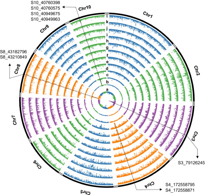
Circular plot from EigenGWAS for Ev1 (a), Ev4 (b), Ev5 (c) and Ev10 (d) based on 509 landrace maize populations, from EnvGWAS on three traits of maximum temperature (tmax; e), minimum temperature (tmin; f), averaged temperature (tavg; g), solar radiation (srad; h), vapour pressure (vapr; i), soil pH at 5 cm depth (ph5; j), rainfall (prec; k) from the monthly long‐term average (1970–2000), and from GWAS on popping versus nonpopping (l). The highlighted SNP S3_79126245, which was annotated as “stop lost,” was in the common region significantly associated with Ev1 in EigenGWAS, and tmax, tmin, tavg and vapr in EnvGWAS. The highlighted SNPs S4_172558795 and S4_172558871 were significantly associated with Ev10 in EigenGWAS, and tmax, tmin, tavg and vapr in EnvGWAS. The highlighted SNPs S8_43182796 and S8_43210849 were significantly associated with Ev4 in EigenGWAS, and tmax, tmin, tavg and vapr in EnvGWAS. SNPs S10_40760398, S10_40760575, S10_40949675 and S10_40949963 were associated with Ev5 in EigenGWAS, and srad in EnvGWAS. Ev1, Ev4, Ev5 and Ev10 are the first, fourth, fifth and tenth eigenvectors, each of which was used as phenotype for the single‐marker association study based on nearly 355,442 markers in EigenGWAS [Colour figure can be viewed at http://wileyonlinelibrary.com]

Figure 7.

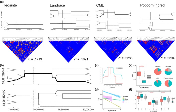
Bifurcation diagram for haplotypes on SNP locus S3_79126245 in the four maize types and pairwise linkage disequilibrium plot with r ² for 2 Mb based on 655,440 data sets around S3_79126245 (a) and in the whole data set (b), extended haplotype homozygosity (EHH) plot for haplotypes on the S3_79126245 locus (c), Ev1 and S3_79126245 genotypes in the four maize types (d), boxplot for Ev1 based on the genotypes of S3_79126245 and allele frequencies at S3_79126245 in the four maize types (e), and the allele frequency distribution of S3_79126245 in three traits related to temperature (f) [Colour figure can be viewed at http://wileyonlinelibrary.com]

3.5. Gene annotation for the SNPs under selection

The annotation conducted on the 65,540 SNP tGBS data and 355,442 SNP imputed data showed that 48.76% and 59.12% of the maize genome respectively is in the intergenic region, and 7.54% and 3.89% respectively is genic (Figure 8a,b). This is consistent with the B73 genome where 6% of the maize genome is genic (Schnable et al. 2009) and a substantial proportion of loci (i.e., 78.00%) associated with phenotypic variation is found in intergenic regions (Li et al., 2012; Mei, Stetter, Gates, Stitzer, & Ross‐Ibarra, 2018; Wallace et al., 2014). Therefore, the tGBS SNPs alone were broadly representative of the genomic distribution of markers. Compared with the original genotypic data, enrichment of particular genomic annotations from EigenGWAS and EnvGWAS in the imputed data is higher in intergenic regions (85.92% and 66.67%; Figure 8c,d). For the two methods, 7.67% and 20.76% of SNPs were in the gene upstream and downstream regions, 5.75% and 9.40% SNPs were in the intron regions, respectively, and fewer than 4% were in exon, splice sites, utr3 prime and utr5 prime regions (Figure 8 and Tables S5 and S6). In total, 146 and 1941 known genes were mapped by the significant SNPs from EigenGWAS and EnvGWAS, respectively, most of which are involved in metabolic and cellular process in gene ontology analysis (Tables S9 and S10).

Figure 8.

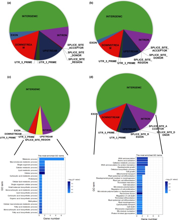
Gene annotation for the original data set (65,540 SNPs) (a), imputed data set (355,442 SNPs) (b), significant SNPs identified by EigenGWAS (c) and EnvGWAS (d) on different types of chromatin, and the top 20 enriched Gene Ontology terms found by functional enrichment analysis for the 146 genes identified by EigenGWAS (c) and 1,941 genes identified by EnvGWAS (d) [Colour figure can be viewed at http://wileyonlinelibrary.com]

3.6. Popping loci related to adaptation

In total, 1,776 significant popping‐related loci, distributing on seven chromosomes, were identified (Figure 6 and Table S11); chromosome 2 (i.e., 1,434 SNPs) had the highest number of significant loci, while chromosomes 3 and 5 (i.e., two SNPs each) had the lowest. S1_103188845 on chromosome 1 was identified as the most significant locus (p = 3.21e‐9). A few annotated popping‐related genes could be found on regulatory regions (i.e., intron, upstream, downstream and 5′ untranslated region). For example, GRMZM2G031802 on chromosome 2 was an endoplasmic reticulum (ER) lumen protein retaining receptor, and GRMZM2G071582 on chromosome 6 was a ZAC, which is a putative calcium‐dependent lipid‐binding (CaLB domain) family protein. The orthologous gene of GRMZM2G071582 in Arabidopsis is AT4G21160.1 which belongs to the calcium‐dependent ARF‐type GTPase activating protein family, and in rice is LOC_Os06g40704.1, which is a stromal membrane‐associated protein. This implies that the popping characteristic could be affected by cellular structure and cell membrane formation. It was worth noting that no popping‐related loci overlapped with the loci identified by EigenGWAS. Compared with significant loci identified by EnvGWAS, almost all the popping‐related loci were associated with ph5 (i.e., 1,285) and prec (i.e., 1,587) distributed on chromosomes 1 and 2; 485 popping‐related loci distributed on chromosomes 1, 2 and 7 were associated with vapr; 173 popping‐related loci on chromosomes 1 and 2 were associated with temperature; and no locus was detected related to srad (Table S12).

4. DISCUSSION

4.1. Large‐scale panel to investigate maize genomic regions under selection

Previous reports employed only a limited number of maize accessions to identify potential adaptation and domestication signals. For example, 56 maize accessions including 30 improved lines, 19 landraces and seven wild relatives were used to investigate how often domestication traits were artificially selected (Lai, Yan, Lu, & Schnable, 2018); 62 Chinese elite inbred lines revealed post‐domestication selection of LEAFY genes (Yang et al., 2014); and 75 wild, landrace and improved maize lines identified several genes with stronger signals of selection than those previously shown to underlie major morphological changes (Hufford et al., 2012). In contrast, 1,143 maize materials collected from 20 countries worldwide were used in the study. This diverse collection covered different ecological zones including tropical highland, lowland, sub/midaltitude and temperate maize materials (Figure 1), and comprised 764 heterozygous landraces and 379 inbred lines. LD decayed rapidly (Figure S5), and the PCA combining HapMap V3 and the 1,143 maize accessions indicated that the 1,143 individuals had the broad genetic divergence for tropical adaptation, covering the regions of predomestication and domestication of Zea mays (Figure S4). These findings indicate that this panel provides a large effective population size and high levels of gene flow in the species, and thus was well suited to study evolutionary adaptation.

4.2. EigenGWAS to detect the selection loci

Selection and adaptation often occur without obvious phenotypic change, suggesting a “bottom‐up” strategy, in which the selection signal is diffused across the genome. F _ST scan, the conventional strategy for exploring signatures of selection, requires the predefinition of subpopulations. Gage et al. (2018) assayed genetic differences using selection statistics XP‐EHH, XP‐CLR and F _ST. Hufford et al. (2012) identified selection signals by XP‐CLR. Lai et al. (2018) identified many “classic” domestication genes through mapping of quantitative trait loci (QTL) in biparental populations derived from wild/domesticated crosses and showed the signatures of parallel selection by XP‐CLR. In this study, we mapped selection loci across the maize genome, employing eigenvector as a phenotype in EigenGWAS, incorporating the definition of subpopulations in a data‐driven manner. Highly significant signals were found on chromosome 3 under Ev1 and Ev4, on chromosome 8 under Ev5, on chromosome 10 under Ev5 and Ev6, on chromosome 2 under Ev7, on chromosome 1 under Ev8, and on chromosome 5 under Ev9 (Figure 5). EigenGWAS well replicated the three regions previously identified, and novel previously unreported loci were also found, providing clues to the global adaptation of maize, and demonstrating the effectiveness of EigenGWAS in finding loci under selection.

In theory, given n eigenvectors, we could perform EigenGWAS on more than the first 10 eigenvectors utilized here. Selection of the number of eigenvectors for analysis could depend upon the significance of the eigenvalue, the overall contribution to genetic variation and discernible association of eigenvectors with known variables such as phenotype, specific adaptation or growing environment. The statistical significance of an eigenvalue could be conducted with a Tracy–Widom test (Tracy & Widom, 1994). The result could then be used to determine the eigenvectors used for analysis. In addition to in silico validation using existing data resources, functional validation in future breeding programmes could be explored for the newly identified loci/regions.

An eigenvalue represents the mean genetic variation captured, whereas λ_GC of the EigenGWAS on the corresponding eigenvector indicates the median of the variation. As an analogue, the difference between eigenvalue and λ_GC is equivalent to the difference between the mean and a median of a population, implying the existence of strong selection, either a natural selection sweep, or artificial selection during breeding or domestication. Much larger differences between eigenvalues and λ_GC were observed in these maize materials (Table 1) than that observed in human populations (e.g., 100.14 vs. 103.72, nearly identical to the difference between the largest eigenvalue and its corresponding λ_GC; table 1 in Chen et al., 2016). This implies possible selection sweeps during maize domestication and adaptation, rather than genetic drift.

4.3. EnvGWAS to detect selection loci

The EnvGWAS used here link precise geographical, climate and soil data for landrace collection sites (called as GIS data for simplicity), with genomic data for each collection (Figure 6 and Figure S14) (Navarro et al., 2017), providing complementary methods to comprehensively decipher the genomic loci/region related to adaptation across the whole genome. Since the GIS data are highly correlated with crop adaptation and selection, they are also highly correlated with population structure, and therefore there is potential confounding between the effects of GIS variables and the underlying population structure. When GIS data were used as phenotype in EnvGWAS, methods based on a mixed model including either only a kinship matrix or both the kinship and the population structure matrix showed very limited associations (Navarro et al., 2017), indicating that these models lower the false‐positive discovery rate but also significantly raise the false‐negative discovery rate. To limit these effects, a simple GLM was used in this study to perform EnvGWAS (Navarro et al., 2017).

4.4. Polygenic adaptation model of maize

Up to now, many functionally characterized genes in maize that underlie phenotypic changes during the domestication have been identified through simple sequence repeat (SSR) markers, SNP chips, GBS and resequencing data (Gage et al., 2018; Lai et al., 2018; Tian et al., 2009). In this study, tGBS with highly accurate genotypic data was first applied to uncover the polygenic domestication and adaptation scheme in maize. Although many selection signatures had been detected before, it remains difficult to fully explain the maize selection and adaptation process and its molecular mechanism. Thus, it is necessary and important to uncover the architecture of selection signatures to understand maize breeding and adaptation (Gage et al., 2018; Hufford et al., 2012; Lai et al., 2018). As Boyle, Li, and Pritchard (2017) have pointed out, species generally adapt by small allele frequency shifts of many causal variants across the genome, emphasizing the polygenic nature of evolution. This is also true for maize adaptation shown by Stetter, Thornton, and Ross‐Ibarra (2018) and in this study. Ten maize regions were first found under selection. Most of the candidate genes had been found in regulatory regions, such as intergenic, intron, upstream and downstream of genes (Table S6). Six SNPs were implicated in changing gene transcription and translation, including loss of start codon, and loss, gain or retention of stop codon. For five genes (i.e., GRMZM2G427685, GRMZM2G357034, GRMZM2G101250, GRMZM2G701576, GRMZM2G425583), no functional annotation was available (Table 2). Three regions were associated with more than one eigenvector, namely SR2.1, SR3.1 and SR10 (Table 2 and Table S5). These probably underwent selection at multiple times during the domestication, breeding and adaptation processes, as reflected in statistically orthogonal eigenvectors (Shlens, 2005). Most of the 13 regions under selection were covered by high marker densities. Uneven SNP distribution among the genome was the result of imputation based on LD (Figure S5). In this case, we were able to narrow the target regions down to some extent.

4.5. Breeding implications and future perspectives

In this study, genomic variations were called by alignment to the only available reference genome (B73). Some, possibly significant, diversity represented by loci not present in the temperate reference was therefore not included in the analysis. It is important and useful to recall SNPs using a tropical reference genome, once a comprehensive version is available, to capture more representative genomic variation. An additional limitation is the breadth of diversity present in the panel representing temperate germplasm; although the 1,143 maize accessions used in this study cover a wide genetic diversity, they still under‐represent the breadth of genetic diversity of HapMap3 (Figure S4) due in part to the small sample size of maize accessions collected from the temperate zone and the breeding selection bias incurred in the use of inbreds of this adaptation.

Results of annotation showed that 48.76% of SNPs in the tGBS data and 59.12% of SNPs in the imputation data map to intergenic regions, while SNP mapping to genic content reflect 7.54% and 3.89% of SNPs, respectively. The distribution of SNPs within the panel evaluated is consistent with the B73 genome where 6% of the maize genome is genic (Schnable et al. 2009), and the high proportion of loci (i.e., 78.00%) associated with phenotypic variation found in intergenic regions in the maize genome (Li et al., 2012; Mei et al., 2018; Wallace et al., 2014). Compared with the original genotypic data, the enrichment of particular genomic annotations from EigenGWAS and EnvGWAS gave a higher number of significant SNPs in intergenic regions—i.e., 85.92% and 66.67%, respectively (Figure 8). In humans and several model animals, most of the GWAS signals map to noncoding regions and potentially point to noncoding variants (Celniker et al., 2009; Dunham et al., 2012; Stamatoyannopoulos et al., 2012; Zhang & Lupski, 2015); and Hindorff et al. (2009) found that most human transcriptionally active sites were found to be located in noncoding regions. Combining GWAS with expression profiling across several thousand individuals to identify both regulatory regions and their effects on phenotype, and including them in prediction models will not only enhance our understanding of basic genetics, but also help breeders to craft better crops.

The reported adaptation loci in the literature have limited applications in breeding, while this is not true in our study. For SNP locus S2_95391165, the alternative S2_95391165‐G haplotype was longer and more abundant than the reference S2_95391165‐A haplotype in Figure S7, indicating that the alternative allele was selected and fixed, and more adaptive to the environment. Opposing selection directions were found in five other haplotypes (Figures S8–S12). The haplotype with reference allele in SR5 shows a very different adaptation pattern. Temperature has a selection preference on the reference haplotype in SR3.1. These results offer potential to help breeders better understand the implication of the genomic footprint on crop adaptation and response to climate change and explore in a more targeted manner exotic germplasm sources containing variation in these genomic regions novel to their own germplasm. We are currently extending this and genomic prediction‐based approaches to whole germplasm bank genomic and GIS data to identify genomic regions and accessions of highest breeding relevance.

AUTHOR SUMMARY

Human population genetic studies infer that adaptation in quantitative traits often occurs through subtle shifts in allele frequencies at many loci, a process called polygenic adaptation. In crop plants the genomic patterns of morphological and physiological changes responding to adaptation to variable environments, cultivation and human use are poorly understood due in part to the limited sample sizes used in studies (<100 in maize for example) and difficulty in separating the signals of adaptation from genetic drift. We evaluated the genomic landscape of 1,143 diverse maize accessions using high‐density genotypic data. Through acombination of genomic data, long term‐climate data, soil dat and population genetic and quantitative genetic approaches we identified regions under selection for adaptive response. Ten selection regions are first reported, and 146 genes mostly in gene regulatory regions are enriched. These regions are promising candidates for further targeted selection of beneficial alleles during maize breeding. Combining large‐scale genomic and ecological data in this diverse maize panel, we demonstrate the polygenic adaptation model of maize, which will facilitate the targeted exploration for adaptive variation of value in the development of new elite cultivars adapted to changing environmental conditions in the face of climate change.

Supporting information

 

 

Li J, Chen G‐B, Rasheed A, et al. Identifying loci with breeding potential across temperate and tropical adaptation via EigenGWAS and EnvGWAS. Mol Ecol. 2019;28:3544–3560. 10.1111/mec.15169

DATA AVAILABILITY STATEMENT

Genotypic, passport and GIS information for the maize accessions is available from http://hdl.handle.net/11529/10548183.

REFERENCES

- Beissinger, T. M. , Hirsch, C. N. , Vaillancourt, B. , Deshpande, S. , Barry, K. , Buell, C. R. , … de Leon, N. (2014). A genome‐wide scan for evidence of selection in a maize population under long‐term artificial selection for ear number. Genetics, 196(3), 829–840. 10.1534/genetics.113.160655 [DOI] [PMC free article] [PubMed] [Google Scholar]
- Bindea, G. , Mlecnik, B. , Hackl, H. , Charoentong, P. , Tosolini, M. , Kirilovsky, A. , … Galon, J. (2009). ClueGO: A Cytoscape plug‐in to decipher functionally grouped gene ontology and pathway annotation networks. Bioinformatics, 25(8), 1091–1093. 10.1093/bioinformatics/btp101 [DOI] [PMC free article] [PubMed] [Google Scholar]
- Bosse, M. , Spurgin, L. G. , Laine, V. N. , Cole, E. F. , Firth, J. A. , Gienapp, P. , … Slate, J. (2017). Recent natural selection causes adaptive evolution of an avian polygenic trait. Science, 358(6361), 365–368. 10.1126/science.aal3298 [DOI] [PubMed] [Google Scholar]
- Boyle, E. A. , Li, Y. I. , & Pritchard, J. K. (2017). An expanded view of complex traits: from polygenic to omnigenic. Cell, 169(7), 1177–1186. 10.1016/j.cell.2017.05.038 [DOI] [PMC free article] [PubMed] [Google Scholar]
- Browning, B. L. , & Browning, S. R. (2016). Genotype imputation with millions of reference samples. The American Journal of Human Genetics, 98(1), 116–126. 10.1016/j.ajhg.2015.11.020 [DOI] [PMC free article] [PubMed] [Google Scholar]
- Browning, S. R. , & Browning, B. L. (2007). Rapid and accurate haplotype phasing and missing‐data inference for whole‐genome association studies by use of localized haplotype clustering. The American Journal of Human Genetics, 81(5), 1084–1097. 10.1086/521987 [DOI] [PMC free article] [PubMed] [Google Scholar]
- Celniker, S. E. , Dillon, L. A. L. , Gerstein, M. B. , Gunsalus, K. C. , Henikoff, S. , Karpen, G. H. , … Waterston, R. H. (2009). Unlocking the secrets of the genome. Nature, 459(7249), 927 10.1038/459927a [DOI] [PMC free article] [PubMed] [Google Scholar]
- Chang, C. C. , Chow, C. C. , Tellier, L. C. , Vattikuti, S. , Purcell, S. M. , & Lee, J. J. (2015). Second‐generation PLINK: Rising to the challenge of larger and richer datasets. Gigascience, 4, 7 10.1186/s13742-015-0047-8 [DOI] [PMC free article] [PubMed] [Google Scholar]
- Chen, G. B. , Lee, S. H. , Zhu, Z. X. , Benyamin, B. , & Robinson, M. R. (2016). EigenGWAS: Finding loci under selection through genome‐wide association studies of eigenvectors in structured populations. Heredity, 117(1), 51–61. 10.1038/hdy.2016.25 [DOI] [PMC free article] [PubMed] [Google Scholar]
- Cingolani, P. , Platts, A. , Wang, L. L. , Coon, M. , Nguyen, T. , Wang, L. , … Ruden, D. M. (2012). A program for annotating and predicting the effects of single nucleotide polymorphisms, SnpEff: SNPs in the genome of Drosophila melanogaster strain w1118; iso‐2; iso‐3. Fly, 6(2), 80–92. 10.4161/fly.19695 [DOI] [PMC free article] [PubMed] [Google Scholar]
- Devlin, B. , & Roeder, K. (1999). Genomic control for association studies. Biometrics, 55(4), 997–1004. 10.1111/j.0006-341X.1999.00997.x [DOI] [PubMed] [Google Scholar]
- Dunham, I. , Kundaje, A. , Aldred, S. F. , Collins, P. J. , Davis, C. , Doyle, F. , … ENCODE Project Consortium (2012). An integrated encyclopedia of DNA elements in the human genome. Nature, 489(7414), 57–74. 10.1038/nature11247 [DOI] [PMC free article] [PubMed] [Google Scholar]
- Elshire, R. J. , Glaubitz, J. C. , Sun, Q. , Poland, J. A. , Kawamoto, K. , Buckler, E. S. , & Mitchell, S. E. (2011). A robust, simple genotyping‐by‐sequencing (GBS) approach for high diversity species. PLoS ONE, 6(5), e19379 10.1371/journal.pone.0019379 [DOI] [PMC free article] [PubMed] [Google Scholar]
- Fick, S. E. , & Hijmans, R. J. (2017). WorldClim 2: New 1‐km spatial resolution climate surfaces for global land areas. International Journal of Climatology, 37(12), 4302–4315. 10.1002/joc.5086 [DOI] [Google Scholar]
- Field, Y. , Boyle, E. A. , Telis, N. , Gao, Z. , Gaulton, K. J. , Golan, D. , … Pritchard, J. K. (2016). Detection of human adaptation during the past 2000 years. Science, 354(6313), 760–764. 10.1126/science.aag0776 [DOI] [PMC free article] [PubMed] [Google Scholar]
- Gage, J. L. , White, M. R. , Edwards, J. , Kaeppler, S. , & de Leon, N. (2018). Selection signatures underlying dramatic male inflorescence transformation during modern hybrid maize breeding. Genetics, 210(3), 1125–1138. [DOI] [PMC free article] [PubMed] [Google Scholar]
- Gaut, B. S. , Seymour, D. K. , Liu, Q. , & Zhou, Y. (2018). Demography and its effects on genomic variation in crop domestication. Nature Plants, 4(8), 512–520. 10.1038/s41477-018-0210-1 [DOI] [PubMed] [Google Scholar]
- Gautier, M. , & Vitalis, R. (2012). rehh: An R package to detect footprints of selection in genome‐wide SNP data from haplotype structure. Bioinformatics, 28(8), 1176–1177. 10.1093/bioinformatics/bts115 [DOI] [PubMed] [Google Scholar]
- Glaubitz, J. C. , Casstevens, T. M. , Lu, F. , Harriman, J. , Elshire, R. J. , Sun, Q. , & Buckler, E. S. (2014). TASSEL‐GBS: A high capacity genotyping by sequencing analysis pipeline. PLoS ONE, 9(2), e90346 10.1371/journal.pone.0090346 [DOI] [PMC free article] [PubMed] [Google Scholar]
- Grossman, S. R. , Shylakhter, I. , Karlsson, E. K. , Byrne, E. H. , Morales, S. , Frieden, G. , … Sabeti, P. C. (2010). A composite of multiple signals distinguishes causal variants in regions of positive selection. Science, 327(5967), 883–886. 10.1126/science.1183863 [DOI] [PubMed] [Google Scholar]
- Hanson, M. A. , Gaut, B. S. , Stec, A. O. , Fuerstenberg, S. I. , Goodman, M. M. , Coe, E. H. , & Doebley, J. F. (1996). Evolution of anthocyanin biosynthesis in maize kernels: The role of regulatory and enzymatic loci. Genetics, 143(3), 1395–1407. [DOI] [PMC free article] [PubMed] [Google Scholar]
- Harberd, N. P. , & Freeling, M. (1989). Genetics of dominant gibberellin‐insensitive dwarfism in maize. Genetics, 121(4), 827–838. [DOI] [PMC free article] [PubMed] [Google Scholar]
- Hengl, T. , Mendes de Jesus, J. , Heuvelink, G. B. M. , Ruiperez Gonzalez, M. , Kilibarda, M. , Blagotić, A. , … Kempen, B. (2017). SoilGrids250m: Global gridded soil information based on machine learning. PLoS ONE, 12(2), e0169748 10.1371/journal.pone.0169748 [DOI] [PMC free article] [PubMed] [Google Scholar]
- Hindorff, L. A. , Sethupathy, P. , Junkins, H. A. , Ramos, E. M. , Mehta, J. P. , Collins, F. S. , & Manolio, T. A. (2009). Potential etiologic and functional implications of genome‐wide association loci for human diseases and traits. Proceedings of the National Academy of Sciences, 106(23), 9362–9367. 10.1073/pnas.0903103106 [DOI] [PMC free article] [PubMed] [Google Scholar]
- Hufford, M. B. , Xu, X. , van Heerwaarden, J. , Pyhäjärvi, T. , Chia, J.‐M. , Cartwright, R. A. , … Ross‐Ibarra, J. (2012). Comparative population genomics of maize domestication and improvement. Nature Genetics, 44(7), 808–U118. 10.1038/ng.2309 [DOI] [PMC free article] [PubMed] [Google Scholar]
- Irish, E. E. , & Nelson, T. M. (1993). Development of tassel seed 2 inflorescences in maize. American Journal of Botany, 292–299. 10.1002/j.1537-2197.1993.tb13802.x [DOI] [Google Scholar]
- Jones, F. C. , Grabherr, M. G. , Chan, Y. F. , Russell, P. , Mauceli, E. , Johnson, J. , … Kingsley, D. M. (2012). The genomic basis of adaptive evolution in threespine sticklebacks. Nature, 484(7392), 55–61. 10.1038/nature10944 [DOI] [PMC free article] [PubMed] [Google Scholar]
- Kim, K.‐W. , Bennison, C. , Hemmings, N. , Brookes, L. , Hurley, L. L. , Griffith, S. C. , … Slate, J. (2017). A sex‐linked supergene controls sperm morphology and swimming speed in a songbird. Nature Ecology & Evolution, 1(8), 1168–1176. 10.1038/s41559-017-0235-2 [DOI] [PubMed] [Google Scholar]
- Lai, X. , Yan, L. , Lu, Y. , & Schnable, J. (2018). Largely unlinked gene sets targeted by selection for domestication syndrome phenotypes in maize and sorghum. The Plant Journal, 93(5), 843–855. 10.1111/tpj.13806 [DOI] [PubMed] [Google Scholar]
- Lasky, J. R. , Upadhyaya, H. D. , Ramu, P. , Deshpande, S. , Hash, C. T. , Bonnette, J. , … Morris, G. P. (2015). Genome‐environment associations in sorghum landraces predict adaptive traits. Science Advances, 1(6), e1400218 10.1126/sciadv.1400218 [DOI] [PMC free article] [PubMed] [Google Scholar]
- Letunic, I. , & Bork, P. (2016). Interactive tree of life (iTOL) v3: An online tool for the display and annotation of phylogenetic and other trees. Nucleic Acids Research, 44, W242–245. 10.1093/nar/gkw290 [DOI] [PMC free article] [PubMed] [Google Scholar]
- Li, X. , Zhu, C. , Yeh, C.‐T. , Wu, W. , Takacs, E. M. , Petsch, K. A. , … Yu, J. (2012). Genic and nongenic contributions to natural variation of quantitative traits in maize. Genome Research, 22(12), 2436–2444. 10.1101/gr.140277.112 [DOI] [PMC free article] [PubMed] [Google Scholar]
- Mei, W. , Stetter, M. G. , Gates, D. J. , Stitzer, M. C. , & Ross‐Ibarra, J. (2018). Adaptation in plant genomes: Bigger is different. American Journal of Botany, 105(1), 16–19. 10.1002/ajb2.1002 [DOI] [PubMed] [Google Scholar]
- Novembre, J. , Johnson, T. , Bryc, K. , Kutalik, Z. , Boyko, A. R. , Auton, A. , … Bustamante, C. D. (2008). Genes mirror geography within Europe. Nature, 456, 98–101. 10.1038/nature07331 [DOI] [PMC free article] [PubMed] [Google Scholar]
- Ott, A. , Liu, S. Z. , Schnable, J. C. , Yeh, C. T. , Wang, K. S. , & Schnable, P. S. (2017). tGBS® genotyping‐by‐sequencing enables reliable genotyping of heterozygous loci. Nucleic Acids Research, 45(21), e178 10.1093/nar/gkx853 [DOI] [PMC free article] [PubMed] [Google Scholar]
- Palaisa, K. , Morgante, M. , Tingey, S. , & Rafalski, A. (2004). Long‐range patterns of diversity and linkage disequilibrium surrounding the maize Y1 gene are indicative of an asymmetric selective sweep. Proceedings of the National Academy of Sciences of the United States of America, 101(26), 9885–9890. 10.1073/pnas.0307839101 [DOI] [PMC free article] [PubMed] [Google Scholar]
- Parolo, S. , Lacroix, S. , Kaput, J. , & Scott‐Boyer, M.‐P. (2017). Ancestors’ dietary patterns and environments could drive positive selection in genes involved in micronutrient metabolism—the case of cofactor transporters. Genes & Nutrition, 12(1), 28 10.1186/s12263-017-0579-x [DOI] [PMC free article] [PubMed] [Google Scholar]
- Price, A. L. , Patterson, N. J. , Plenge, R. M. , Weinblatt, M. E. , Shadick, N. A. , & Reich, D. (2006). Principal components analysis corrects for stratification in genome‐wide association studies. Nature Genetics, 38(8), 904–909. 10.1038/ng1847 [DOI] [PubMed] [Google Scholar]
- Romay, M. C. , Millard, M. J. , Glaubitz, J. C. , Peiffer, J. A. , Swarts, K. L. , Casstevens, T. M. , … Gardner, C. A. (2013). Comprehensive genotyping of the USA national maize inbred seed bank. Genome Biology, 14(6), R55 10.1186/Gb-2013-14-6-R55 [DOI] [PMC free article] [PubMed] [Google Scholar]
- Romero Navarro, J. A. , Willcox, M. , Burgueño, J. , Romay, C. , Swarts, K. , Trachsel, S. , … Buckler, E. S. (2017). A study of allelic diversity underlying flowering‐time adaptation in maize landraces. Nature Genetics, 49(3), 476–480. 10.1038/ng.3784 [DOI] [PubMed] [Google Scholar]
- Sabeti, P. C. , Varilly, P. , Fry, B. , Lohmueller, J. , Hostetter, E. , Cotsapas, C. , … Lander, E. S. (2007). Genome‐wide detection and characterization of positive selection in human populations. Nature, 449(7164), 913–918. 10.1038/nature06250 [DOI] [PMC free article] [PubMed] [Google Scholar]
- Schnable, P. S. , Ware, D. , Fulton, R. S. , Stein, J. C. , Wei, F. , Pasternak, S. , … Minx, P. (2009). B73 maize genome: complexity, diversity, and dynamics. Science, 326(5956), 1112–1115. 10.1371/journal.pone.0169748 [DOI] [PubMed] [Google Scholar]
- Shlens, J. (2005). A tutorial on principal component analysis. Retrieved from http://www.snl.salk.edu/~shlens/pub/notes/pca.pdf [Accessed 8 August 2008]. [Google Scholar]
- Stamatoyannopoulos, J. A. , Snyder, M. , Hardison, R. , Ren, B. , Gingeras, T. , Gilbert, D. M. , … Adams, L. B. (2012). An encyclopedia of mouse DNA elements (Mouse ENCODE). Genome Biology, 13(8), 418 10.1186/gb-2012-13-8-418 [DOI] [PMC free article] [PubMed] [Google Scholar]
- Stephan, W. (2016). Signatures of positive selection: From selective sweeps at individual loci to subtle allele frequency changes in polygenic adaptation. Molecular Ecology, 25(1), 79–88. 10.1111/mec.13288 [DOI] [PubMed] [Google Scholar]
- Stetter, M. G. , Thornton, K. , & Ross‐Ibarra, J. (2018). Genetic architecture and selective sweeps after polygenic adaptation to distant trait optima. PLOS Genetics, 14(11), e1007794 10.1371/journal.pgen.1007794 [DOI] [PMC free article] [PubMed] [Google Scholar]
- Swarts, K. , Li, H. , Romero Navarro, J. A. , An, D. , Romay, M. C. , Hearne, S. , … Bradbury, P. J. (2014). Novel methods to optimize genotypic imputation for low‐coverage, next‐generation sequence data in crop plants. The Plant Genome, 7(3). 10.3835/plantgenome2014.05.0023 [DOI] [Google Scholar]
- Thornsberry, J. M. , Goodman, M. M. , Doebley, J. , Kresovich, S. , Nielsen, D. , & Buckler, E. S. IV (2001). Dwarf8 polymorphisms associate with variation in flowering time. Nature Genetics, 28(3), 286–289. 10.1038/90135 [DOI] [PubMed] [Google Scholar]
- Tian, F. , Stevens, N. M. , & Buckler, E. S. 4th (2009). Tracking footprints of maize domestication and evidence for a massive selective sweep on chromosome 10. Proceedings of the National Academy of Sciences of the United States of America, 106(Suppl 1), 9979–9986. 10.1073/pnas.0901122106 [DOI] [PMC free article] [PubMed] [Google Scholar]
- Tracy, C. A. , & Widom, H. (1994). Level‐spacing distributions and the Airy kernel. Communications in Mathematical Physics, 159(1), 151–174. 10.1007/BF02100489 [DOI] [Google Scholar]
- Turner, T. L. , Bourne, E. C. , Von Wettberg, E. J. , Hu, T. T. , & Nuzhdin, S. V. (2010). Population resequencing reveals local adaptation of Arabidopsis lyrata to serpentine soils. Nature Genetics, 42(3), 260–263. 10.1038/ng.515 [DOI] [PubMed] [Google Scholar]
- Vielle‐Calzada, J.‐P. , de la Vega, O. M. , Hernández‐Guzmán, G. , Ibarra‐Laclette, E. , Alvarez‐Mejía, C. , Vega‐Arreguín, J. C. , … Herrera‐Estrella, L. (2009). The Palomero genome suggests metal effects on domestication. Science, 326(5956), 1078–1078. [DOI] [PubMed] [Google Scholar]
- Vigouroux, Y. , McMullen, M. , Hittinger, C. T. , Houchins, K. , Schulz, L. , Kresovich, S. , … Doebley, J. (2002). Identifying genes of agronomic importance in maize by screening microsatellites for evidence of selection during domestication. Proceedings of the National Academy of Sciences of the United States of America, 99(15), 9650–9655. 10.1073/pnas.112324299 [DOI] [PMC free article] [PubMed] [Google Scholar]
- Voight, B. F. , Kudaravalli, S. , Wen, X. , & Pritchard, J. K. (2006). A map of recent positive selection in the human genome. PLoS Biology, 4(3), e72 10.1371/journal.pbio.0040072 [DOI] [PMC free article] [PubMed] [Google Scholar]
- Wallace, J. G. , Bradbury, P. J. , Zhang, N. , Gibon, Y. , Stitt, M. , & Buckler, E. S. (2014). Association mapping across numerous traits reveals patterns of functional variation in maize. PLoS Genetics, 10(12), e1004845 10.1371/journal.pgen.1004845 [DOI] [PMC free article] [PubMed] [Google Scholar]
- Wang, H. , Studer, A. J. , Zhao, Q. , Meeley, R. , & Doebley, J. F. (2015). Evidence that the origin of naked kernels during maize domestication was caused by a single amino acid substitution in tga1 . Genetics, 200(3), 965–974. 10.1534/genetics.115.175752 [DOI] [PMC free article] [PubMed] [Google Scholar]
- Wang, R.‐L. , Stec, A. , Hey, J. , Lukens, L. , & Doebley, J. (1999). The limits of selection during maize domestication. Nature, 398(6724), 236 10.1038/18435 [DOI] [PubMed] [Google Scholar]
- Whipple, C. J. , Kebrom, T. H. , Weber, A. L. , Yang, F. , Hall, D. , Meeley, R. , … Jackson, D. P. (2011). grassy tillers1 promotes apical dominance in maize and responds to shade signals in the grasses. Proceedings of the National Academy of Sciences of the United States of America, 108(33), E506–512. 10.1073/pnas.1102819108 [DOI] [PMC free article] [PubMed] [Google Scholar]
- Whitt, S. R. , Wilson, L. M. , Tenaillon, M. I. , Gaut, B. S. , & Buckler, E. S. (2002). Genetic diversity and selection in the maize starch pathway. Proceedings of the National Academy of Sciences of the United States of America, 99(20), 12959–12962. 10.1073/pnas.202476999 [DOI] [PMC free article] [PubMed] [Google Scholar]
- Wills, D. M. , Whipple, C. J. , Takuno, S. , Kursel, L. E. , Shannon, L. M. , Ross‐Ibarra, J. , & Doebley, J. F. (2013). From many, one: Genetic control of prolificacy during maize domestication. PLoS Genetics, 9(6), e1003604 10.1371/journal.pgen.1003604 [DOI] [PMC free article] [PubMed] [Google Scholar]
- Wright, S. (1951). The genetical structure of populations. Annals of Eugenics, 15(4), 323–354. [DOI] [PubMed] [Google Scholar]
- Wu, Y. , San Vicente, F. , Huang, K. , Dhliwayo, T. , Costich, D. E. , Semagn, K. , … Babu, R. (2016). Molecular characterization of CIMMYT maize inbred lines with genotyping‐by‐sequencing SNPs. Theoretical and Applied Genetics, 129(4), 753–765. 10.1007/s00122-016-2664-8 [DOI] [PMC free article] [PubMed] [Google Scholar]
- Yang, Z. , Zhang, E. , Li, J. , Jiang, Y. , Wang, Y. , Hu, Y. , & Xu, C. (2014). Analyses of sequence polymorphism and haplotype diversity of LEAFY genes revealed post‐domestication selection in the Chinese elite maize inbred lines. Molecular Biology Reports, 41(2), 1117–1125. 10.1007/s11033-013-2958-8 [DOI] [PubMed] [Google Scholar]
- Zhang, F. , & Lupski, J. R. (2015). Non‐coding genetic variants in human disease. Human Molecular Genetics, 24(R1), R102–R110. [DOI] [PMC free article] [PubMed] [Google Scholar]
Associated Data
This section collects any data citations, data availability statements, or supplementary materials included in this article.
Supplementary Materials