

Abstract
Advances in species distribution modeling continue to be driven by a need to predict species responses to environmental change coupled with increasing data availability. Recent work has focused on development of methods that integrate multiple streams of data to model species distributions. Combining sources of information increases spatial coverage and can improve accuracy in estimates of species distributions. However, when fusing multiple streams of data, the temporal and spatial resolutions of data sources may be mismatched. This occurs when data sources have fluctuating geographic coverage, varying spatial scales and resolutions, and differing sources of bias and sparsity. It is well documented in the spatial statistics literature that ignoring the misalignment of different data sources will result in bias in both the point estimates and uncertainty. This will ultimately lead to inaccurate predictions of species distributions. Here, we examine the issue of misaligned data as it relates specifically to integrated species distribution models. We then provide a general solution that builds off work in the statistical literature for the change‐of‐support problem. Specifically, we leverage spatial correlation and repeat observations at multiple scales to make statistically valid predictions at the ecologically relevant scale of inference. An added feature of the approach is that addressing differences in spatial resolution between data sets can allow for the evaluation and calibration of lesser‐quality sources in many instances. Using both simulations and data examples, we highlight the utility of this modeling approach and the consequences of not reconciling misaligned spatial data. We conclude with a brief discussion of the upcoming challenges and obstacles for species distribution modeling via data fusion.
Keywords: black‐throated blue warbler, change of support, Data integration for population models Special Feature, integrated species distribution modeling, occupancy modeling, spatial modeling
Introduction
Determining how species respond to changing environmental conditions is fundamental to sound management and species conservation (Yoccoz et al. 2001). Accomplishing this requires leveraging empirical evidence to inform and ultimately validate decision making. This need for data‐driven decision making has motivated significant advances in the ability to collect and store spatially and temporally referenced data. At the same time there has been an influx in the development and application of methods that integrate multiple streams of data. These new data‐integration approaches seek to exhaust all available data sources to model species distributions while explicitly accounting for differences among data types (Dorazio 2014, Fithian et al. 2015, Giraud et al. 2016, Pacifici et al. 2017, Coron et al. 2018). The advantages of combining multiple data sources in integrated species distribution models (ISDMs) include increased spatial coverage, bias reduction and overall improvement in estimator accuracy (Dorazio 2014, Fithian et al. 2015, Giraud et al. 2016, Pacifici et al. 2017). Several authors have put forth different approaches for integrating different data sources, typically when one source is collected through standardized surveys and the other source is not (Fletcher et al. 2019, Miller et al. 2019). As a result, we now have a range of methods that leverage information across different data types (Dorazio 2014, Pacifici et al. 2017, Zipkin et al. 2017), among multiple species (Giraud et al. 2016, Thorson et al. 2016, 2017), and among neighboring locations by incorporating spatial correlation (Thorson et al. 2017). As data becomes more available and easier to access the propensity to combine data will only increase, as will the demand to apply it rigorously to inform decision making.
In light of the increased interest in ISDMs, it is essential to explore the implications that come with combining different data sources. As with all species distribution modeling the goal is to correlate observations of individual species with environmental layers that are driving the observed patterns of occurrence. In some cases, the focus will be on large geographic areas or on species that are difficult to sample. Alternative data sources can fill in gaps that might occur in data collection and improve inference (Pacifici et al. 2017, Fletcher et al. 2019, Miller et al. 2019). Integrated species distribution models can increase precision and reduce bias in certain settings (Pacifici et al. 2017) and are flexible enough to incorporate a wide range of auxiliary data sources (Fletcher et al. 2019, Miller et al. 2019). Despite this, two major problems need to be addressed when fusing multiple streams of data. The first problem is to ensure that the ISDM rigorously combines each data source so that relevant and valid statistical inference is possible. The second is to reconcile spatial and temporal observations properly when they are collected at multiple differing spatial and temporal resolutions. The first problem has already received significant attention (Fletcher et al. 2019, Miller et al. 2019). The result is a range of flexible approaches that have been developed to integrate multiple data sources rigorously (Pacifici et al. 2017, Fletcher et al. 2019). The second problem, however, has not been formally addressed for ISDMs in the ecological literature. This stands in contrast to significant coverage given to the topic in the spatial statistics literature, where it is often referenced as the general change of support (COS) problem (Mugglin et al. 2000, Gelfand et al. 2001, Gotway and Young 2002, 2007, Wikle and Berliner 2005, Young and Gotway 2007, Berrocal et al. 2010a,b, Ren and Banerjee 2013, Reich et al. 2014, Parker et al. 2015, Kim and Berliner 2016).
Before exploring the challenges of combining data sources and COS we first need to understand COS as it relates to a single data source. Here, we briefly describe three general COS problems. We encourage the reader to explore the topic more thoroughly (Gelfand et al. 2001, Gotway and Young 2002); Journal of the Royal Statistical Society, Series A, Volume 164 Issue 1 is dedicated to the topic. Generally, COS arises from three causes: (1) spatial or temporal misalignment, (2) modifiable areal unit problem (MAUP), and (3) the ecological fallacy problem. It is important to recognize that the effect of COS can exist in relation to either the response variable (e.g., counts, occurrences), the covariates driving the response (e.g., landcover, elevation), or both.
First, data may be “misaligned” either spatially or temporally (Mugglin et al. 2000, Cressie and Wikle 2015) meaning that data may come from different classifications or partitions of parcels of land or from different years or seasons. Take for example the case where a predictor variable (e.g., elevation) is measured at one spatial scale (e.g., county) and another variable (e.g., human population density) is measured at a different spatial scale (e.g., zip code). Our interest may be in using both covariates to explain variation, in say, abundance. However, the misalignment of the covariate information needs to be reconciled to make proper inference (Mugglin et al. 2000). The same will hold for temporal mismatch wherein one covariate may be measured at a different temporal resolution (e.g., annually) than a second covariate (e.g., daily) and the differences must be recognized (Cressie and Wikle 2015). The problem of misalignment also occurs when the response variable (e.g., counts, presence/absence data) is mismatched with the covariate information either spatially (e.g., counts occur at different spatial scale than covariate) or temporally (e.g., covariate information, say land cover, comes from different year than counts were collected).
The second problem classified under COS is referred to as the modifiable areal unit problem (MAUP) in the geography and statistics literature (Gotway and Young 2002). Modifiable areal unit problem is essentially two separate problems: spatial aggregation and the grouping effect. Spatial aggregation is the process of grouping data into increasingly larger geographic units. This might occur when covariate information is aggregated or grouped to a larger scale to match another covariate or response variable (Latimer et al. 2006) or response variables (e.g., counts) are summarized at increasingly larger geographic scales (e.g., collected at point, summarized to county level). Spatial aggregation will change inferences for estimated parameters. The second problem of MAUP, the grouping effect, occurs when there are differences in the size, shape, or formation of the geographic units (Gotway and Young 2002). Grouping effects have been studied extensively in ecology for some time (Turner 1989, Levin 1992).
A third challenge, “ecological fallacy,” is often listed separately from MAUP, but also can be considered a special case of MAUP. Ecological fallacy deals with the case where the underlying individual response to a covariate differs from the response estimated from grouping the individuals (Gotway and Young 2002, Bradley et al. 2016, 2017). The result is that conclusions based on an analysis using fine‐resolution data differ from analyses that are conducted using an aggregate or summary of the fine‐resolution data (Gotway and Young 2002). “Downscaling” is often used to address this problem in the environmental and remote sensing fields (Bradley et al. 2017). Often the most difficult piece is identifying which variables are responsible for significantly altering the results when data are scaled up or aggregated from individual level to group level (Gotway and Young 2002).
In all three cases, notable bias can occur if it is not properly handled, and choosing different scales to conduct the analysis results in different magnitudes of error (Bradley et al. 2017). Bias can occur not only in estimating the mean and variance of parameters of interest, but extends to any statistic that is estimated at multiple scales (Waller and Gotway 2004, Bradley et al. 2017). The consequences of ignoring COS are hard to predict, and they can result in severe biases.
Although the statistical literature is rich with examples of COS (Gotway and Young 2002) it generally remains unaddressed in species distribution modeling. Several authors note that COS occurs when species presence/absence data that are referenced to point locations and environmental data used to predict occurrence are typically referenced to grid cells (Latimer et al. 2006, Finley et al. 2014). Another example is when location errors arising from georeferenced covariate information that is summarized or aggregated to a grid cell (Hefley et al. 2017). (Latimer et al. 2006) describe a solution as either working at the scale of the responses by assigning the environmental data to that level or alternatively working at the grid cell level by scaling up the response data to match the environmental data. However, this leads to a loss of information from rescaling to match either the level of the response or the level of the environmental data. Ideally we want a method to account for and circumvent the loss of information due to aggregating data formally, and to recognize the variation within and between the aggregated units. The frequency with which COS will occur and associated issues becomes greater when multiple sources of data are combined, as now both the covariate information and auxiliary response data can be from mismatched scales.
The nuances of each type of COS warrants careful consideration of the appropriate solution. A wide range of methods exist (Gotway and Young 2002), with the general goal being to make spatial predictions or estimate variables (covariates or responses) on regions over which they were not measured (Mugglin et al. 2000, Gotway and Young 2002). As (Cressie and Wikle 2015) recommend, the only logical solution is to build models at different scales and evaluate the differences in inference when doing so, ideally first building the model at the finest scale and then aggregating or scaling up to fit additional models. We will apply this general philosophy to COS with multiple data sources as well.
Here we lay out a framework for accommodating COS when combining multiple sources of data in ISDMs. First we describe the theoretical underpinnings of COS in the context of ISDMs, then develop COS extensions to a suite of data fusion models that vary in the level of shared information between data sources (Pacifici et al. 2017). We explore the properties of these models via simulation and apply these methods to our motivating data set on Black‐throated Blue Warblers (Setophaga caerulescens; BTBW) in Pennsylvania, USA (Fig. 1). Our overall objectives are twofold: (1) introduce the concept of COS and demonstrate its relevancy to ISDMs, and (2) identify specific situations when COS most matters and provide recommendations for how it should be handled.
Figure 1.
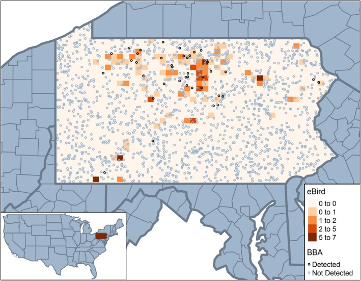
Motivating data sets: Black‐throated Blue Warbler in Pennsylvania, USA. Example of combining two data sources collected at different spatial scales used in integrated species distribution modeling. The first data source is collected at fine‐resolution surveys (Breeding Bird Atlas [BBA]), and the second data source (eBird) is summarized at a coarser resolution. [Color figure can be viewed at https://www.wileyonlinelibrary.com]
Change of Support for Integrated Species Distribution Models
We will use a case study of BTBW in Pennsylvania, USA to demonstrate the challenges of accounting for COS in ISDMs (Fig. 1). Here two different data sources provide useful, yet different information about the distribution of BTBW. The first data source is collected at finer‐resolution standardized surveys across the state (Breeding Bird Atlas point counts), and the second data source (eBird) has been summarized at a coarser resolution to account for data that are not collected at a single point location. Combining these data create a conflict in spatial resolution and necessitates a method that addresses the misalignment. This requires being able to reconcile the misalignment between the two data sources and the differing spatial scales to make inferences about the underlying distribution of BTBW.
Modeling framework
We envision two general approaches to handle misalignment to accommodate COS. The first naive method is a two‐stage approach (we formally define this approach below as the “Covariate” model). The first step consists of imputing the second data source in the spatial locations where the response of the first data source is observed. The prediction could be done in any number of ways depending on the characteristics of the second data source (e.g., presence only, presence–absence, counts) and could be accomplished using any number of appropriate species distribution modeling techniques (Guillera‐Arroita et al. 2015). The second step uses those predicted values as known constants and linear predictors in an ISDM (Dorazio 2014, Fithian et al. 2015, Fletcher et al. 2016, 2019, Pacifici et al. 2017, Miller et al. 2019). However, this approach does not account for uncertainty in the predictions from the second data source during the first step and can result in potentially biased inference. The second general approach, and the one we will focus on here, is a joint‐modeling strategy. In this case, both sources of data are modeled simultaneously. As a result, uncertainty is properly accounted for and propagated through to the predictions of the joint response. Below we describe the framework for joint modeling of ISDMs to account for spatial misalignment.
Species distributions can generally be thought of as a continuous point process that describes the distribution of individuals across a species’ range. The local intensity of the process (i.e., the local probability an individual occurs at any point in space) determines the density of animals across space. Building a statistical model for the distribution requires carefully aggregating the intensity function for a point process to the scale of the data. As with any probability density function of a continuous random variable, the probability of an observation at any single spatial location is zero. As a result, non zero probabilities arise only when considering the number of observations in a spatial region. Therefore, some minimum form of aggregation is required. For example, if a camera trap is placed at location and animals that pass within distance from the camera are recorded, then the region of the survey, , is the circle with center and radius and the expected number of observations in is , which increases with . Given that all observations are made with reference to an area, it is generally difficult to estimate the function for all without simplifying assumptions about its smoothness.
Following much of the literature on species distribution models (SDMs), we specify our model for individual spatial locations (i.e., latitude/longitude) using an inhomogeneous Poisson process (IPP; Warton et al. 2010, Dorazio 2014, Fithian et al. 2015). An IPP is simply a point process where the intensity (i.e., local density of individuals) varies across space. Let be the intensity of an inhomogeneous Poisson process so that the number of individuals in an arbitrary region follows a Poisson distribution with mean
| (1) |
The log‐intensity process can be regressed onto covariates via the model where is a vector of spatial covariates, are the corresponding effects and is the residual spatial process. Several models for the spatial intensity function have been proposed and we discuss three in Appendix S1.
Data Fusion Models with COS
As we noted previously, the focus of our paper is to integrate multiple data sources collected at different spatial resolutions. Assume that data source is available for regions . Consistent with our motivating data example with BTBW in Pennsylvania, we address the case where there are two data sources and (1) the first data source is the number of the sampling occasions in region for which the species was observed, so that ; and (2) that the second data source is the total number of individuals observed in grid cell , so that . The approaches below are easily generalized to other cases. In our analyses we will treat the first data source as the “gold standard.” The data are collected using a systematic sampling design where effort and location are well defined and offer a benchmark for our data integration model. The second data source contains auxiliary data for which we have less confidence and this is reflected in how we formulate models in some cases (Pacifici et al. 2017). We describe the methods below in the context of the discretized model that assumes the true intensity is constant with each fine‐resolution grid cell described above. For our motivating example this model is amenable to implementation in standard software (e.g., OpenBUGS, see available code in Data S1). However, we emphasize that other approaches can also be used in the data‐fusion models developed in this section.
Here we lay out three approaches for data fusion that vary in the degree of influence and reliance on the auxiliary data source (Pacifici et al. 2017) and extend each to allow for COS.
Covariate model
The simplest approach is to use the second data source or a summary of the second data source as a covariate in the model for the first data source (i.e., ad‐hoc two‐stage approach described above). Note that technically there is no modification for COS; instead information from the response is scaled up or matched to the covariate scale and therefore the misalignment is reconciled. We continue to include this model because it is a simple and effective way to address spatial misalignment. In this case, information from the auxiliary data only informs the species distribution model to the extent it can predict data from the second. The model for the first data source is
| (2) |
where is the binary indicator that cell is occupied and is the probability of detection given that the cell is occupied. If the number of individuals in region follows a Poisson distribution with mean defined as in Appendix S1: Eq. S2 then the probability that the number of individuals is zero, i.e., that , is . Therefore the probability that is occupied given is
| (3) |
We use a spatial log‐Gaussian model for the intensity function; therefore each fine‐resolution cell is
| (4) |
where is the vector of covariates, is the corresponding vector of regression coefficients, and is a spatial random effect. By including a summary of the auxiliary data in the covariate vector we use information in both data sources. For example, if fine‐resolution cell falls in coarse resolution cell , then we will use as an element of . As a result, the coarse‐resolution covariate might prove useful for capturing large‐scale spatial patterns, but cannot resolve fine‐scale variation. (Pacifici et al. 2017) show this is a useful model when belief in the second data source is low or uncertain as nothing is assumed about the auxiliary data source.
We chose to estimate the vector of spatial random effects using a conditional autoregressive prior (CAR; Banerjee et al. 2014), but note that any model for a continuous spatial process could be used with a few modifications. However, we chose to use the CAR model because of its easy implementation in available software (e.g., BUGS). The CAR model can be motivated using the full conditional specification of given the value of the process at all other cells,
where is the mean of at the cells adjacent to cell and the two spatial dependence parameters and determine the strength of spatial dependence and conditional variance, respectively. These full conditional distributions lead to the joint multivariate normal distribution
| (5) |
where is the diagonal matrix with diagonal element equal to and is the adjacency matrix with element equals one if cells and are adjacent and zero otherwise. We denote this as .
Shared model
An alternative to the simple naive approach is to treat both data sources as outcomes of the same underlying distribution and relate them directly to the shared underlying inhomogeneous point process. In this case there is a single underlying species distribution, but each data source is allowed to have its own model that describes the observation process (i.e., the probability of collecting a given observation conditional on the true number of individuals within a given location). All outcomes are taken to be conditionally independent given the intensities. The joint model is
where and are additive and multiplicative bias terms, respectively and represent the degree of relatedness between the two data sources (e.g., when the second data source is completely uninformative). The intensity surface is modeled as in (4) except without as an element of . This is the typical joint‐likelihood approach found in many applications of integrated population models and ISDMs (Dorazio 2014, Fletcher et al. 2016, 2019, Zipkin et al. 2017). It assumes that the secondary data source is of high quality and/or information is available to model the sources of bias and variability (e.g., false positives, variable sampling effort).
Correlation model
A second alternative to fully modeling the joint likelihood is to specify separate, but correlated, underlying processes for the two data sources. The idea here is to estimate two separate species distributions, one with each data set, while allowing the two distributions to be correlated. If they are perfectly correlated, information is completely shared across the two distribution models. If the correlation is <1, then information is shared in proportion to the strength of correlation. This allows us to relax the reliance on the auxiliary data source necessary for joint‐likelihood approaches while still permitting information to be shared between the sources of data (Pacifici et al. 2017). Let be the Poisson intensity function for data source and be the aggregated intensity for process . As with the shared model, the data are conditionally independent given the Poisson intensities,
Both processes are defined on the same fine grid grid cells, with
| (6) |
where is the vector of covariates; is the corresponding vector of regression coefficients for data type ; and is a spatial random effect. The spatial random effects are modeled using a multivariate CAR model (Banerjee et al. 2014), defined by its full conditional distributions
where is the mean of at the cells adjacent to cell ; controls the strength of spatial dependence; and the covariance matrix controls the dependence between and . This model allows for the processes underlying two data sources to be correlated. Thus each data source informs predictions from the other, but in an indirect manner. As a result, there is a reduced burden for the auxiliary data being of equally reliable to the first data source.
Simulation Study: Aggregating Spatial Covariates with a Single Data Source
Now that we have formally defined COS in ISDMs we want to explore one of the most common challenges that researchers first face when fitting SDMs: how to use spatial covariates that have been collected at different spatial scales. Below we describe a brief simulation study to evaluate the effect of aggregating spatial covariates with a single data source. In this simulation the true intensity surface is generated on a fine grid of grid cells . Data are generated on grid cells , where each cell contains regular grid of of the fine‐resolution cells, with denoting the indices of the fine‐resolution cells in so that (e.g., Appendix S1: Fig. S1a for ). We first simulate the spatial random effects and covariate . The true intensity is then set to with and . The data for is then generated as where with detection probability . Data are simulated with aggregation level either or spatial correlation of the covariate equal either or . For all combinations of these settings we simulate 500 data sets.
For each simulated data set we fit two models. The first model (“naive”) ignores COS and fits a standard spatial occupancy model using observations where the log intensity in cell is , where is the average of over and the spatial effects follow a CAR prior defined via the adjacency matrix of . The second model (“COS”) is the COS model used to generate the data wherein we account for COS by modeling the process at the same fine resolution that we generated the data (instead of using the average as in the naive model). Both models assume priors , , and . Models are fit in OpenBUGS using 10,000 MCMC samples after a burn‐in period of 2,500 iterations (see Data S1 for code). For each model and each data set we compute the posterior distribution of the slope , and present the bias and mean square error of the posterior mean and empirical coverage of 90% intervals averaged over the 500 data sets in Table 1.
Table 1.
Simulation study results: Single data source with spatially aggregated covariate: Here we are exploring the consequences of rescaling a covariate with a single data source. The data generation depends on the dimension of the aggregate cells () and the CAR spatial dependence of the covariate process (); the two methods are the naive method that models the process only at the course resolution and the change of the support (COS) method that models the process on the fine resolution. Methods are compared using Bias, mean squared error (MSE) and coverage of 90% intervals for the covariate effect parameter,
| Settings | Bias | MSE | Coverage | ||||||
|---|---|---|---|---|---|---|---|---|---|
|
|
|
Naive | COS | Naive | COS | Naive | COS | ||
| 2 | 0.50 | 0.69 | 0.14 | 1.57 | 0.58 | 0.89 | 0.88 | ||
| 0.99 | 1.02 | 0.25 | 1.80 | 0.39 | 0.79 | 0.86 | |||
| 3 | 0.50 | 0.34 | 0.09 | 1.77 | 1.27 | 0.94 | 0.92 | ||
| 0.99 | 1.07 | 0.41 | 2.11 | 0.76 | 0.84 | 0.85 | |||
The naive method that ignores COS is positively biased in all cases. The bias and MSE are the largest in the cases with a highly correlated covariate process (). Although the COS method does not completely eliminate the bias, it is greatly reduced especially in the cases with spatial correlation therefore highlighting the need to account for COS even with mismatched covariate and response data.
Simulation Study: ISDMs with and without COS
To evaluate the newly developed COS ISDMs fully, we conduct a simulation study to determine the conditions in which fusing data sources with different spatial resolutions improves estimates, and compare the efficiency of various ways to account for the COS. We generated data from the shared model on a 20 × 20 rectangular grid. The data are originally generated on the same grid as the true process; i.e., . The observed data in cell is a function of the latent spatial process . The true binary occupancy status is generated as . The fine‐scale data are then sampled as
| (7) |
where N = 5, the detection probability is either 0.2 or 0.5 and is the offset for the second data source. The latent intensities are simulated as , where is generated from the CAR model (with rook neighbors) with mean zero, variance parameter , spatial dependence parameter set to either 0.50 or 0.99. The first data source, , is observed for all grid cells; the second data source, , is only observed as aggregated counts over ( is either 2 or 4) rectangular grids, denoted for coarse‐resolution grid cell . Appendix S1: Fig. S1 plots one realization with , , and .
For each combination of , , and we generate 100 data sets and fit the following models:
Single: The second data source is ignored
Covariate: The covariate model with is used as a covariate
Shared: The joint model for and
Correlation: The correlation model for and
Shared—no COS: is assumed to represent one central fine scale grid cell and the data are analyzed using the shared method without COS (Appendix S1: Fig. S1d)
Correlation—no COS: is assumed to represent one central fine‐scale grid cell and the data are analyzed using the correlation method without COS (Appendix S1: Fig. S1d)
Each model is fit using OpenBUGS with three chains each with 20,000 iterations and the first 5,000 iterations discarded as burn‐in (see Data S1 for code). We used uninformative priors for all parameters and evaluated convergence using the Gelman–Rubin statistic and examining trace plots.
For each method and each data set we compute the posterior probability that the fine‐resolution cells are occupied, denoted , and the declaration that the cell is occupied, denoted if and if . Methods are evaluated using the Brier Score (BS) which is a proper score function to evaluate predictive performance for binary outcomes (Gneiting and Raftery 2007, Pacifici et al. 2016; lower is better) and classification accuracy (CA) averaged over cells,
| (8) |
where is the true occupancy status generated from the CAR model. Table 2 reports the median Brier score and classification accuracy across the 100 data sets for each method and each simulation scenario.
Table 2.
Simulation study results: accounting for change of support (COS) in integrated species distribution models (ISDMs). Here we are interested in evaluating the consequences of ignoring COS in fitting ISDMs. The data generation depends on the dimension of the aggregate cells (), the detection probability (), and the Multivariate Conditional Autoregressive (MCAR) model dependence parameter ; the five methods are the model that uses only one source of data (“Single”), the three change‐of‐support methods (“Shared,” “Correlation,” and “Covariate”), and the data fusion methods that ignore change of support (“Shared—no COS” and “Correlation—no COS”). The Brier score and classification accuracy are the median of 100 simulated datasets for each scenario
| Scenario | Settings | Change of support | No COS | ||||||||
|---|---|---|---|---|---|---|---|---|---|---|---|
|
|
|
|
Single | Shared | Correlation | Covariate | Shared | Correlation | |||
| (a) Brier score | |||||||||||
| 2 | 0.2 | 0.50 | 0.141 | 0.126 | 0.135 | 0.132 | 0.133 | 0.137 | |||
| 2 | 0.2 | 0.99 | 0.117 | 0.101 | 0.110 | 0.102 | 0.108 | 0.117 | |||
| 2 | 0.5 | 0.50 | 0.018 | 0.018 | 0.018 | 0.018 | 0.019 | 0.018 | |||
| 2 | 0.5 | 0.99 | 0.017 | 0.016 | 0.016 | 0.016 | 0.017 | 0.017 | |||
| 4 | 0.2 | 0.50 | 0.138 | 0.135 | 0.139 | 0.138 | 0.137 | 0.143 | |||
| 4 | 0.2 | 0.99 | 0.118 | 0.110 | 0.116 | 0.112 | 0.112 | 0.119 | |||
| 4 | 0.5 | 0.50 | 0.018 | 0.018 | 0.018 | 0.018 | 0.018 | 0.018 | |||
| 4 | 0.5 | 0.99 | 0.017 | 0.016 | 0.017 | 0.016 | 0.017 | 0.017 | |||
| (b) Classification accuracy | |||||||||||
| 2 | 0.2 | 0.50 | 0.775 | 0.802 | 0.794 | 0.789 | 0.791 | 0.786 | |||
| 2 | 0.2 | 0.99 | 0.820 | 0.852 | 0.833 | 0.848 | 0.840 | 0.823 | |||
| 2 | 0.5 | 0.50 | 0.981 | 0.981 | 0.981 | 0.981 | 0.980 | 0.981 | |||
| 2 | 0.5 | 0.99 | 0.982 | 0.982 | 0.982 | 0.981 | 0.980 | 0.981 | |||
| 4 | 0.2 | 0.50 | 0.777 | 0.784 | 0.786 | 0.780 | 0.781 | 0.780 | |||
| 4 | 0.2 | 0.99 | 0.821 | 0.836 | 0.824 | 0.831 | 0.834 | 0.820 | |||
| 4 | 0.5 | 0.50 | 0.981 | 0.981 | 0.981 | 0.981 | 0.981 | 0.981 | |||
| 4 | 0.5 | 0.99 | 0.982 | 0.982 | 0.982 | 0.981 | 0.981 | 0.981 | |||
| (c) CPU times (min) | |||||||||||
| 2 | 0.2 | 0.50 | 2.57 | 2.75 | 4.54 | 2.56 | 2.54 | 4.27 | |||
Including the second data source only shows substantial improvement compared to the single‐data‐source model when the grid cells are small () and detection is low (). With large grid cells the aggregated data are too coarse to provide useful spatial information, and with high detection the first data sources provide sufficient information to produce precise maps, because we included data from all cells within the area for this data source. Strong spatial correlation improves classification accuracy for all methods, but the second data source provides roughly the same increase in precision regardless of the spatial correlation.
Focusing on the two cases with and where including the second data source is useful, the results are fairly robust to the COS method. The two simplest COS methods are the covariate model and the naive methods that include the aggregated data as a data point without accounting for COS. These two simple models perform comparably to the more sophisticated shared and correlation models. The average run times for these methods (Table 2c) are approximately 50% less than the full correlation model. In summary, these two methods provide simple and effective means of accommodating COS in ISDMs.
Case Study: Black‐throated Blue Warblers in Pennsylvania
We next apply the data fusion models with and without COS on a data set for BTBW in Pennsylvania, USA. Our goal is to examine the real‐world consequences of ignoring COS and to make recommendations for modeling. We have two data sets collected from two different sources. We further subsample these data at different spatial scales (i.e., observations are assigned to cells of increasing sizes) to understand the utility of incorporating COS into ISDMs.
The first data set we use includes point count survey data collected as part of the second Pennsylvania Breeding Bird Atlas (BBA data; Wilson et al. 2012). During a 5‐yr period from 2005 to 2009, 33,846 point count surveys were conducted across the state of Pennsylvania. An even distribution of points was achieved by randomly selecting eight roadside locations within each standard 1/24‐degree latitude by 1/16‐degree longitude blocks used for the atlas (Grid 1; Table 3). Point counts occurred during morning hours in the peak breeding season (last week of May through the end of June). Observers recorded singing males of all species during a 6 min 15 s survey. Observations were divided into five 75‐s intervals and whether the bird was located less than or greater than 150 m from the observer. In our analysis we used all observations of singing male BTBW. We excluded observations >150 m from the observer.
Table 3.
Spatial Resolutions for change of support (COS). We evaluated four different spatial resolutions to explore the consequences of spatial misalignment in integrated species distribution models (ISDMs). Two different data sources were used, which came from different spatial resolutions. Breeding Bird Atlas data came from the finest resolution (Grid 1), and eBird data were summarized for each of the other resolutions. We used these mismatches in scale to highlight the utility of accommodating COS in ISDMs
| Spatial resolution | Grid size (degrees) | Grid size (km2) |
|---|---|---|
| Grid 1 | 1/24 × 1/16 | 24.3 |
| Grid 2 | 1/12 × 1/8 | 97.5 |
| Grid 3 | 1/3 × 1/2 | 1,553.6 |
| Grid 4 | 2/3 × 1 | 6,230.5 |
Our second data set consists of eBird observations (Sullivan et al. 2009). We filtered eBird records to only include observations during the same 5‐yr period (2005–2009) and only included records during the breeding season (late May–July). Records that did not include measures of survey effort were excluded. A subset of the BBA data was entered into the eBird database. To avoid duplication these records were also removed for analysis. A total of 4,937 checklists were included in our analyses. eBird data were summarized at three different resolutions, not including the original scale of the BBA data (Grid 1; Table 3).
Preliminary analyses found that percent forest cover has a positive relationship with the occurrence of Black‐throated Blue Warbler. We therefore include this covariate in all of the models to understand the consequences of spatial misalignment on the ability to estimate the covariate effects. In addition we summarize the second data source (eBird) in two different ways, first we take the sum of the eBird counts for a particular grid size and average it across all of the BBA cells at Grid 1 within the larger grid (denoted by “Avg” following the model name). Second, we explore the effects of an ad hoc approach wherein we reconcile the misalignment by matching the grids for all of the data (referenced by “Scaled” following the model name). That is, we scale up the BBA data to match the eBird grid. This is to mimic the case where nothing is known about the location of the finer‐resolution data and instead scale it up to match the second data source.
To evaluate the effects of ignoring vs. accommodating COS fully, we fit the data fusion models described in the Data Fusion Models with COS section with and without COS to 20% of the BBA data and compare the results with a model fit to all of the BBA data. The full BBA data set (33,846 points across Pennsylvania) has excellent geographic coverage, and by subsetting this data set we were able to explore the contrast in performance among the approaches.
Case Study Results
Overall models ignoring COS perform poorly compared to models incorporating COS. Fig. 2 shows the estimated occupancy probability across data fusion models and whether COS was incorporated. All of the models incorporating COS had smaller credible intervals and were centered around the value estimated by the full BBA data set. Models ignoring COS and using both data sources equally (Shared) resulted in most estimates that are much higher than the full data set, although this is not the case when the covariate is aggregated up to match the eBird grid size (models with “Scaled” after name). The covariate model using the averaged covariate across all of the finer‐resolution cells (models with “Avg” after name) performs well compared to more complex models (shared and correlation).
Figure 2.
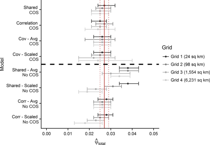
Estimates of total occupancy probabilities from integrated species distribution models (ISDMs) incorporating change of support (COS) vs. ignoring COS at four different spatial resolutions. The second data source is aggregated at different spatial scales (Grids 1–4) to mimic different degrees of spatial misalignment. The solid red line represents the point estimate of occupancy probability from the full, primary data source (Breeding Bird Atlas [BBA]) with uncertainty (95% CI: dotted red line). “Avg” and “Scaled” in model names (y axis) refer to the method used to summarize the second data source (see case study description for complete details). COS models are separated from No COS models by a horizontal dashed line. [Color figure can be viewed at https://www.wileyonlinelibrary.com]
Individual site‐level estimates of show similar results. Appendix S1: Fig. S2 plots the estimates when both data sources are at grid level 1. Models that do not account for COS tend to oversmooth the estimated occurrence probabilities compared to the full data set. This becomes more pronounced as the degree of spatial misalignment increases (Fig. 3). Again the covariate model performs competitively with the more complex shared COS model and outperforms the models ignoring COS.
Figure 3.
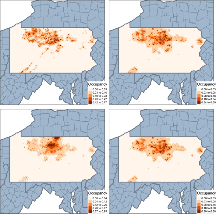
Occupancy estimates from the single, covariate, shared—No change of support (COS), and shared COS models with eBird summarized at coarsest resolution (grid size = 6,231 sq km): The plot in the upper left panel shows the distribution of occupancy for the full, primary data source (Breeding Bird Atlas [BBA]). Clockwise, the plot in the upper right panel shows the results from the covariate model, shared COS, and shared—no COS in bottom left. [Color figure can be viewed at https://www.wileyonlinelibrary.com]
We can compare the performance of the two models using different approaches to summarizing the second data source in the covariate model. Fig. 4 shows the performance at grid level 2 and Appendix S1: Fig. S4 depicts the performance at grid level 4. Here we can see how the second approach (scaling up the first data source to match the second) clearly averages over the spatial variation at a finer scale and oversmooths the predictions.
Figure 4.
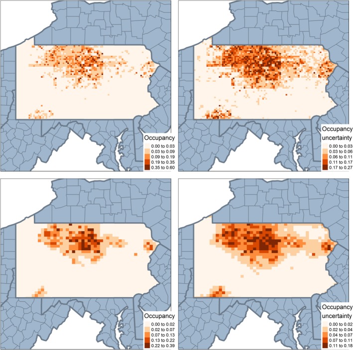
Occupancy estimates from the covariate model with second data source summarized in two different ways at grid level 2 (98 sq km): The plot in the upper left panel shows the results from the covariate model (“Cov‐Avg”) with the second data source averaged across all smaller sites, with uncertainty on upper right panel. The lower left panel shows results from the covariate model (“Cov‐Scaled”) with the covariates summarized by scaling up the covariate values from the finer resolution to match the larger grid size. [Color figure can be viewed at https://www.wileyonlinelibrary.com]
Fig. 5 shows the differences in estimated effects of percent forest cover when ignoring COS vs. accommodating it for data fusion models. The full data set (denoted by “Single”) shows a positive relationship with per cent forest cover and occurrence probabilities. This relationship is not as clear with the data fusion models, although this is probably due to the reduction in data (full data set vs. 20% of the data being used for all of the data fusion models). Overall, the models incorporating COS tend to perform less variably and have reduced uncertainty estimates. It is also important to note as the degree of misalignment increases the amount of uncertainty increases as well. Models using the second data source summarized at Grids 3 and 4 have highly variable and uncertain estimates relative to models using the second data source summarized at Grids 1 and 2. This pattern is especially pronounced for the models ignoring COS.
Figure 5.
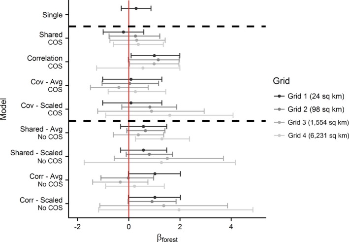
Estimated effect of % forest cover under data fusion models that incorporate or ignore spatial misalignment in integrated species distribution models (ISDMs). The second data source is aggregated at different spatial scales (Grids 1–4) to mimic different degrees of spatial misalignment. Single model is provided as a reference to the estimated effect using full Breeding Bird Atlas (BBA) data set. “Avg” and “Scaled” in model names (y axis) refer to method used to summarize the second data source (see case study description for complete details). Solid red vertical line placed at 0 provided to visualize significance of the effect of % forest cover on occupancy probability. Dashed black horizontal lines used to separate models using one data source and change of support (COS) and No COS models. [Color figure can be viewed at https://www.wileyonlinelibrary.com]
Discussion
We present the first comprehensive treatment of spatial misalignment for ISDMs in the ecological literature. Within the spatial statistics literature, it is well known that spatial alignment matters when making predictions (Gelfand et al. 2001, Gotway and Young 2002). Thus it is not surprising that our results show that COS matters and when unaddressed leads to biased parameter estimates when combining data sources to build ISDMs. Data integration methods have shown both utility and future promise to improve our inferences about species distributions as well as population and community dynamics (Zipkin and Saunders 2018, Fletcher et al. 2019, Miller et al. 2019). Although much of the current effort has focused on the development of estimators for different data types, (Dorazio 2014, Fletcher et al. 2016, Pacifici et al. 2017), a parallel effort is needed to deal with scale and alignment in building models.
Our results highlight cases where not accounting for COS may be especially prone to introduce bias and reduce accuracy in results. We found bias and misclassification errors to be greatest when spatial correlation was high and when detection was low. Error due to COS was also greater when the relationship between distribution and the environment is defined by small‐scale processes. For example, greater bias would be expected in our estimated relationships for BTBW if abundance was more correlated to local forest cover within 100 m of a location rather than at the landscape scale measured when values are taken for whole grid cells. In general, summarizing covariate information to match the grid size of observations smooths over important spatial variation, and can result in a loss of power to detect relationships and fine‐scale trends. The likely result is that the strength of ecological relationships are underestimated. This is not a result unique to data integration methods, but is the case any time we fit models at coarse scales and ignore the COS issue.
We explored three general approaches to data integration, which we refer to as a shared, correlation, and covariate models for integrating two data sources (Pacifici et al. 2017). The covariate modeling approach provides a simple and efficient method for dealing with COS when it occurs between two data sets. By using data collected at a coarser scale as a covariate, it is possible to estimate the relationship of fine‐level processes while sufficiently accounting for information loss due to spatial misalignment. The extent of the spatial misalignment will define the extent to which the two data sets are correlated. As demonstrated previously (Pacifici et al. 2017, Miller et al. 2019), the covariate approach also provides a flexible method to deal with other observational errors, such as misidentification and misspecification of locations.
What we refer to as a shared modeling approach or a joint‐likelihood approach leads to the greatest preservation of information when COS is accounted for while combining data sources. Using a shared approach requires that both data sets be of high quality and that COS can accurately be modeled between the two data sets. If this is the case, then information from both data sets are placed on equal footing and are used to model a shared (or joint) underlying process. In contrast, when it is difficult to specify the COS, the covariate approach performed relatively well, especially when the primary data set can be specified at a fine scale.
Our results point to some recommendations for SDMs in general, not just when data integration is used. Misalignment between covariate resolution and the size of the grid cell for which responses are modeled is not unique to integrated methods (Latimer et al. 2006). One insight from our specific results is that fine‐scale relationships between covariate and species distribution are more affected by ignoring misalignment than coarse‐scale relationships. This suggests that covariates such as average climate, which tend to follow smoother gradients, especially in nonmountainous regions, should be relatively robust to spatial misalignment. Alternatively, estimating fine‐scale habitat relationships, such as the effect of forest cover in a fragmented landscape, will be more sensitive to misalignment. In addition, many of the data sets we use to predict species distributions such as museum records, citizen science data, or even large‐scale designed surveys include large uncertainty about spatial location of where records are located (Dickinson et al. 2010). Therefore, there is a need to understand better how scale influences inferences made from all SDMs (Steenweg et al. 2018).
COS model steps
We are unable to provide general recommendations that are ubiquitous to fitting ISDMs. However, we provide five steps that we believe should be followed when addressing COS in ISDMs.
Define the stochastic model for ecological process at the finest scale or resolution.
Define support for observed data and determine the desired scale for predictions, i.e. scale that conservation and management decisions will be made.
Identify best way to link data sources based on underlying ecological process. Here a second data source may provide a diversity of information including sources of error or effort.
Develop joint model for data sources and the underlying ecological process and conduct inference.
Conduct model evaluation and check for sensitivity (e.g., significant change in results when adding new data sources) specifically when rescaling the data.
Temporal mismatch
Here we have purposely excluded a full evaluation of temporal mismatch because we believe it deserves its own treatment in a separate paper. However, we can provide a few insights into handling temporal mismatch based on our experiences with ISDMs. The first question an analyst must address is whether or not there is interest in a static or dynamic model of species distribution. This question dictates the types of data collected and the temporal resolution necessary to assume that distributional patterns are changing through time. If the analyst is interested in modeling distributional changes via dynamic models, then the temporal resolution of the data must represent the appropriate time scale to allow changes in the distribution at an ecologically relevant scale. When combining multiple sources of data this can present challenges when opportunistic data potentially arises from historic records (e.g., museum records), creating a gap in time. For example, it is common to use presence‐only data that may have originated decades earlier than survey data. In this case the appropriate inference depends on the interpretation of “distribution” in that a coarse time scale suggests a coarser definition of distribution and is akin to results from redefining the response of interest (Guillera‐Arroita et al. 2015). We believe that this definition can be relaxed when interest involves a static distribution of species occurrence, but this is still an important and active area of research to understand fully the implications of temporal mismatch when combining multiple sources of data.
Furthermore, to understand the implications of combining different data sources fully, it is necessary to classify the use of auxiliary data by how it is used to inform SDMs. Similar to integrated population models (IPMs), wherein the goal is to include supplemental data sources that inform specific vital rates that drive populations (Zipkin and Saunders 2018), we can identify the components of SDMs and how integrating new data improves our understanding of distribution and distributional changes in populations. Specifically, we are interested in how additional data sources improve our understanding of the drivers of distributions, and we do this by classifying new sources of data into two categories, spatial and/or temporal, wherein new information can be added. The spatial category can be thought of as including additional observations (presences and/or absences) that modify the geographic footprint of a species, provide information about sampling effort or variation in sampling effort, sources of bias or error (e.g., false positives or false negatives) or that help reduce these sources of error, and uncover or identify relationships with environmental covariates or other species (especially at different spatial scales). Adding temporal information includes observations (presences and/or absences) that modify the geographic range over a temporal scale (e.g., annual or seasonal variation) of interest, or improve our understanding of error and/or sampling effort (similar to spatial), except that which occurs over a temporal scale instead of spatial scale. The classification of how additional data will inform SDMs is a critical step in fully understanding whether it is worth using auxiliary information and how it will help.
Future Directions
As we move forward and the number of opportunities to combine data sources increases we believe future directions for research include the need to explore more fully situations where spatial misalignment has the greatest influence on SDMs. In addition, new applications such as dynamic distribution models are also likely to be affected by COS, specifically because the ability to estimate changes in distribution are dependent on differentiating when local changes did and did not occur, often at a finer scale than the resolution of many data sets (Kery et al. 2013, Zurell et al. 2016). Finally, spatial alignment is not a problem unique to data integration for SDMs. Other integrated models, such as IPMs, will benefit from a better understanding of the effects of spatial misalignment and accounting for COS (Schaub and Abadi 2011, Zipkin et al. 2017).
Supporting information
Acknowledgments
We would like to thanks Steve Beissinger, Brian Inouye, and Elise Zipkin and two anonymous reviewers for helpful comments on earlier drafts of the manuscript.
Pacifici, K. , Reich B. J., Miller D. A. W., and Pease B. S.. 2019. Resolving misaligned spatial data with integrated species distribution models. Ecology 100(6):e02709 10.1002/ecy.2709
Corresponding Editor: Brian D. Inouye.
Editors’ Note: Papers in this Special Feature are linked online in a virtual table of contents at: http://www.wiley.com/go/ecologyjournal
Data Availability
Data are available from GitHub/Zenodo: http://doi.org/10.5281/zenodo.2541844
Literature Cited
- Banerjee, S. , Carlin B. P., and Gelfand A. E.. 2014. Hierarchical modeling and analysis for spatial data. CRC Press, Boca Raton, Florida, USA. [Google Scholar]
- Berrocal, V. J. , Gelfand A. E., and Holland D. M.. 2010a. A bivariate space‐time downscaler under space and time misalignment. Annals of Applied Statistics 4:1942. [DOI] [PMC free article] [PubMed] [Google Scholar]
- Berrocal, V. J. , Gelfand A. E., and Holland D. M.. 2010b. A spatio‐temporal downscaler for output from numerical models. Journal of Agricultural, Biological, and Environmental Statistics 15:176–197. [DOI] [PMC free article] [PubMed] [Google Scholar]
- Bradley, J. R. , Wikle C. K., and Holan S. H.. 2016. Bayesian spatial change of support for count‐valued survey data with application to the American community survey. Journal of the American Statistical Association 111:472–487. [Google Scholar]
- Bradley, J. R. , Wikle C. K., and Holan S. H.. 2017. Regionalization of multiscale spatial processes by using a criterion for spatial aggregation error. Journal of the Royal Statistical Society B 79:815–832. [Google Scholar]
- Coron, C. , Calenge C., Giraud C., and Julliard R.. 2018. Bayesian estimation of species relative abundances and habitat preferences using opportunistic data. Environmental and Ecological Statistics 25:71–93. [Google Scholar]
- Cressie, N. , and Wikle C. K.. 2015. Statistics for spatio‐temporal data. John Wiley & Sons, Hoboken, New Jersey, USA. [Google Scholar]
- Dickinson, J. L. , Zuckerberg B., and Bonter D. N.. 2010. Citizen science as an ecological research tool: challenges and benefits. Annual Review of Ecology, Evolution, and Systematics 41:149–172. [Google Scholar]
- Dorazio, R. M. 2014. Accounting for imperfect detection and survey bias in statistical analysis of presence‐only data. Global Ecology and Biogeography 23:1472–1484. [Google Scholar]
- Finley, A. O. , Banerjee S., and Cook B. D.. 2014. Bayesian hierarchical models for spatially misaligned data in R. Methods in Ecology and Evolution 5:514–523. [Google Scholar]
- Fithian, W. , Elith J., Hastie T., and Keith D. A.. 2015. Bias correction in species distribution models: pooling survey and collection data for multiple species. Methods in Ecology and Evolution 6:424–438. [DOI] [PMC free article] [PubMed] [Google Scholar]
- Fletcher, R. , Hefley T., Robertson E., Zuckerberg B., McCleery R., and Dorazio R.. 2019. A practical guide for combining data to predict species distributions. Ecology 100:e02710. [DOI] [PubMed] [Google Scholar]
- Fletcher, R. J. , McCleery R. A., Greene D. U., and Tye C. A.. 2016. Integrated models that unite local and regional data reveal larger‐scale environmental relationships and improve predictions of species distributions. Landscape Ecology 31:1369–1382. [Google Scholar]
- Gelfand, A. E. , Zhu L., and Carlin B. P.. 2001. On the change of support problem for spatio‐temporal data. Biostatistics 2:31–45. [DOI] [PubMed] [Google Scholar]
- Giraud, C. , Calenge C., Coron C., and Julliard R.. 2016. Capitalizing on opportunistic data for monitoring relative abundances of species. Biometrics 72:649–658. [DOI] [PubMed] [Google Scholar]
- Gneiting, T. , and Raftery A. E.. 2007. Strictly proper scoring rules, prediction, and estimation. Journal of the American Statistical Association 102:359–378. [Google Scholar]
- Gotway, C. A. , and Young L. J.. 2002. Combining incompatible spatial data. Journal of the American Statistical Association 97:632–648. [Google Scholar]
- Gotway, C. A. , and Young L. J.. 2007. A geostatistical approach to linking geographically aggregated data from different sources. Journal of Computational and Graphical Statistics 16:115–135. [Google Scholar]
- Guillera‐Arroita, G. , Lahoz‐Monfort J. J., Elith J., Gordon A., Kujala H., Lentini P. E., McCarthy M. A., Tingley R., and Wintle B. A.. 2015. Is my species distribution model fit for purpose? matching data and models to applications. Global Ecology and Biogeography 24:276–292. [Google Scholar]
- Hefley, T. J. , Brost B. M., and Hooten M. B.. 2017. Bias correction of bounded location errors in presence‐only data. Methods in Ecology and Evolution 8:1566–1573. [Google Scholar]
- Kery, M. , Guillera‐Arroita G., and Lahoz‐Monfort J. J.. 2013. Analysing and mapping species range dynamics using occupancy models. Journal of Biogeography 40:1463–1474. [Google Scholar]
- Kim, Y. , and Berliner L. M.. 2016. Change of spatiotemporal scale in dynamic models. Computational Statistics & Data Analysis 101:80–92. [Google Scholar]
- Latimer, A. M. , Wu S., Gelfand A. E., and Silander J. A.. 2006. Building statistical models to analyze species distributions. Ecological Applications 16:33–50. [DOI] [PubMed] [Google Scholar]
- Levin, S. A. 1992. The problem of pattern and scale in ecology: the Robert H. Macarthur award lecture. Ecology 73:1943–1967. [Google Scholar]
- Miller, D. A. , Pacifici K., Sanderlin J., and Reich B. J.. 2019. The recent past and promising future for data integration methods to estimate species’ distributions. Methods in Ecology and Evolution 10.1111/2041-210x.13110 [DOI] [Google Scholar]
- Mugglin, A. S. , Carlin B. P., and Gelfand A. E.. 2000. Fully model‐based approaches for spatially misaligned data. Journal of the American Statistical Association 95:877–887. [Google Scholar]
- Pacifici, K. , Reich B. J., Dorazio R. M., and Conroy M. J.. 2016. Occupancy estimation for rare species using a spatially‐adaptive sampling design. Methods in Ecology and Evolution 7:285–293. [Google Scholar]
- Pacifici, K. , Reich B. J., Miller D. A., Gardner B., Stauffer G., Singh S., McKerrow A., and Collazo J. A.. 2017. Integrating multiple data sources in species distribution modeling: A framework for data fusion. Ecology 98:840–850. [DOI] [PubMed] [Google Scholar]
- Parker, R. J. , Reich B. J., and Sain S. R.. 2015. A multiresolution approach to estimating the value added by regional climate models. Journal of Climate 28:8873–8887. [Google Scholar]
- Reich, B. J. , Chang H. H., and Foley K. M.. 2014. A spectral method for spatial downscaling. Biometrics 70:932–942. [DOI] [PMC free article] [PubMed] [Google Scholar]
- Ren, Q. , and Banerjee S.. 2013. Hierarchical factor models for large spatially misaligned data: A low‐rank predictive process approach. Biometrics 69:19–30. [DOI] [PMC free article] [PubMed] [Google Scholar]
- Schaub, M. , and Abadi F.. 2011. Integrated population models: a novel analysis framework for deeper insights into population dynamics. Journal of Ornithology 152:227–237. [Google Scholar]
- Steenweg, R. , Hebblewhite M., Whittington J., Lukacs P., and McKelvey K.. 2018. Sampling scales define occupancy and underlying occupancy—abundance relationships in animals. Ecology 99:172–183. [DOI] [PubMed] [Google Scholar]
- Sullivan, B. L. , Wood C. L., Iliff M. J., Bonney R. E., Fink D., and Kelling S.. 2009. eBird: A citizen‐based bird observation network in the biological sciences. Biological Conservation 142:2282–2292. [Google Scholar]
- Thorson, J. T. , Ianelli J. N., Larsen E. A., Ries L., Scheuerell M. D., Szuwalski C., and Zipkin E. F.. 2016. Joint dynamic species distribution models: a tool for community ordination and spatio‐temporal monitoring. Global Ecology and Biogeography 25:1144–1158. [Google Scholar]
- Thorson, J. T. , Munch S. B., and Swain D. P.. 2017. Estimating partial regulation in spatiotemporal models of community dynamics. Ecology 98:1277–1289. [DOI] [PubMed] [Google Scholar]
- Turner, M. G. 1989. Landscape ecology: the effect of pattern on process. Annual review of ecology and systematics 20:171–197. [Google Scholar]
- Waller, L. A. , and Gotway C. A.. 2004. Applied spatial statistics for public health data. Volume 368 John Wiley & Sons, Hoboken, New Jersey, USA. [Google Scholar]
- Warton, D. I. , et al. 2010. Poisson point process models solve the “pseudo‐absence problem” for presence‐only data in ecology. Annals of Applied Statistics 4:1383–1402. [Google Scholar]
- Wikle, C. K. , and Berliner L. M.. 2005. Combining information across spatial scales. Technometrics 47:80–91. [Google Scholar]
- Wilson, A. M. , Brauning D. W., and Mulvihill R. S.. 2012. Second atlas of breeding birds in Pennsylvania. Faculty Publications, Gettysburg, Pennsylvania, USA. [Google Scholar]
- Yoccoz, N. , Nichols J. D., and Boulinier T.. 2001. Monitoring of biological diversity in space and time. Trends in Ecology and Evolution 16:446–453. [Google Scholar]
- Young, L. J. , and Gotway C. A.. 2007. Linking spatial data from different sources: the effects of change of support. Stochastic Environmental Research and Risk Assessment 21:589–600. [Google Scholar]
- Zipkin, E. F. , Rossman S., Yackulic C. B., Wiens J. D., Thorson J. T., Davis R. J., and Grant E. H. C.. 2017. Integrating count and detection–nondetection data to model population dynamics. Ecology 98:1640–1650. [DOI] [PubMed] [Google Scholar]
- Zipkin, E. F. , and Saunders S. P.. 2018. Synthesizing multiple data types for biological conservation using integrated population models. Biological Conservation 217:240–250. [Google Scholar]
- Zurell, D. , et al. 2016. Benchmarking novel approaches for modelling species range dynamics. Global Change Biology 22:2651–2664. [DOI] [PMC free article] [PubMed] [Google Scholar]
Associated Data
This section collects any data citations, data availability statements, or supplementary materials included in this article.
Supplementary Materials
Data Availability Statement
Data are available from GitHub/Zenodo: http://doi.org/10.5281/zenodo.2541844