Effect of prolonged acquisition intervals for CT‐perfusion analysis methods in patients with ischemic stroke

Abstract

Introduction

The limited axial coverage of many computed tomography (CT) scanners poses a high risk on false negative findings in cerebral CT‐perfusion (CTP) imaging. Axial coverage may be increased by moving the table back and forth during image acquisition. However, this method often increases the acquisition interval between CT frames, which may influence the CTP analysis. In this study, we evaluated the influence of different acquisition intervals on quantitative perfusion maps and infarct volumes by analyzing patient data with three CTP analysis methods.

Methods

CT‐perfusion data from 25 patients with ischemic stroke were used for this study. The acquisition interval was synthetically reduced from 1 to 5 s before calculating perfusion values, which included cerebral blood flow (CBF), cerebral blood volume (CBV), and mean transit time (MTT). The color scaling of the perfusion was scaled such that the mean perfusion value had the same color‐coding as the mean perfusion in the 1 s reference. Also, infarct core and penumbra volumes (summary map) were calculated using default thresholds of CBV and relative MTT (rMTT). The original, 1 s acquisition interval scan served as the reference standard. A commercial block‐circulant singular value decomposition (bSVD) based method (ISP; Philips Healthcare), a non‐commercial bSVD method, and a non‐linear regression (NLR) model‐based method were evaluated.

Results

Cerebral blood volume values generated with bSVD and NLR were not significantly different from the reference standard, while ISP showed significant differences for acquisition intervals of 3 and 4 s. MTT and CBF values generated with bSVD and ISP were significantly different for all acquisition intervals, whereas NLR did not show any significant differences. Calibrated perfusion maps were able to distinguish healthy from infarcted tissue up to an acquisition interval of 5 s for all methods. The infarct core volumes were significantly different for acquisition intervals of 2 (NLR) and 3 s (bSVD and ISP) or greater. For the penumbra volumes, NLR showed no significant differences, while bSVD and ISP showed significant differences for the 5 s interval and for all intervals, respectively. Visual inspection of the summary maps indicated minor differences between the reference standard and acquisition intervals of 4 s or less (ISP) and 5 s or less (bSVD and NLR).

Conclusion

Altering the acquisition interval may introduce a bias in the perfusion parameters. Calibration of the visualization of the perfusion maps with increasing acquisition intervals allowed distinction between healthy and infarcted tissue. Infarct volumes based on relative MTT can be influenced by the acquisition interval, but visual inspection of the summary maps indicated minor differences between the reference standard and acquisition intervals up to 4 (ISP) and 5 s (bSVD and NLR). Taken together, axial coverage can be increased by prolonging the acquisition interval up to 5 s depending on the perfusion analysis.

Abbreviations

AIF

arterial input function

bSVD

block‐circulant singular value decomposition

CBF

cerebral blood flow

CBV

cerebral blood volume

IRF

impulse response function

ISP

intellispace portal 9; brain perfusion

MTT

mean transit time

NLR

academic perfusion analysis

rMTT

relative MTT map

TAC

time attenuation curve

1. Introduction

Computed Tomography (CT) imaging is used worldwide to identify presence and potential causes of ischemic stroke in patients with suspected stroke.1, 2 CT imaging is quick, widely available, cost‐effective, and has fewer constraints than MRI, which makes CT the preferred imaging modality for the acute stroke setting. The acute stroke imaging protocol usually includes non‐contrast CT, CT‐perfusion (CTP), and CT‐angiography imaging.3

A dynamic contrast‐enhanced CTP scan is typically an acquisition of 1 min that monitors the wash‐in and washout of the iodinated contrast agent in the brain parenchyma. A number of perfusion parameter maps can be inferred from CTP by using kinetic tracer analysis. These parameter maps give a quantitative insight into the perfusion status of the brain and are often used for clinical decision making as they can differentiate between healthy, salvageable (penumbra), and lost (infarct core) brain tissue.4, 5

The accuracy of the CTP analysis may depend on the number of frames that are acquired per series. In current stroke imaging protocols, frames are typically acquired every 1 or 2 s. It is hypothesized that more frames, which require a shorter acquisition interval, would allow more precise monitoring of the contrast passage resulting in more accurate estimations of the perfusion parameters. However, the lowest achievable acquisition interval is limited because of dose and technical restrictions.

Ideally, the CTP scan covers the entire brain, which is possible by using CT scanners that have a sufficient large axial coverage. However, the majority of CT scanners have insufficient axial coverage to cover the brain (usually 4 cm or less). This can cause false negative findings with CTP imaging, since the chosen cross‐sectional images of the brain may not contain the ischemic area(s).6, 7, 8 Several methods (including Jog Mode and Shuttle Mode and dual tracer injections) have been introduced to dynamically acquire an area that is larger than the original axial coverage. These protocols require the patient bed to be shifted or jogged in and out of the gantry. The time it takes for the table to move from one position to another, limits the lowest achievable acquisition interval. Jog Mode, which is available on the 64‐slice IQon spectral CT scanner (Philips Healthcare, Best, the Netherlands), yields a minimum acquisition interval of 3.4 s, whereas 1 or 2 s may be preferred for CTP imaging. The acquisition interval of CTP imaging has been point of discussion in a number of papers, in which discordant findings were presented. Wintermark et al.9 showed that acquisition intervals of up to 4 s could be reached without influencing the quantitative accuracy of CTP by maintaining the signal‐to‐noise ratio by increasing the amount of contrast agent. However, a number of studies observed opposing findings.10, 11, 12 For instance, Wiesmann et al.11 found that the acquisition interval could not be prolonged without compromising the image quality beyond 3 s. Similarly, Kämena et al.10 recommended an interval of 2 s or lower, and Abels et al.12 even recommended a maximum interval of 1 s. Instead of a fixed acquisition interval, Cao et al.13 suggested the use of irregular sampling, since the monitoring of the bolus passage is more important than the remaining tail of the bolus. A possible explanation for these differences between studies is the observed differences in noise levels, due to the differences in acquisition parameters (kVp, mAs, etc.). Interestingly, the reported studies also used different perfusion analysis methods, which may also explain the large differences in the response to prolonged acquisition intervals. Several CTP analysis methods exist such as block‐circulant Singular Value Decomposition (bSVD). In addition to commonly used analysis methods, we have introduced a non‐linear regression‐based perfusion analysis method (NLR), which is able to estimate perfusion parameters maps in a flexible and robust manner in response to noise, tracer delay, and truncation.14 Therefore, NLR is hypothesized to sustain longer intervals than conventional methods.

In an effort to study the feasibility, reliability, and accuracy of Jog Mode in CTP imaging with equal contrast bolus volume, the purpose of this study is to assess the effects of increased acquisition intervals on quantitative perfusion parameters and infarct volumes. Three CTP analysis methods were evaluated: a commercial perfusion analysis method (ISP; Brain Perfusion, IntelliSpace Portal 9, Philips Healthcare, Best, the Netherlands), a non‐commercial bSVD method15 and the NLR method.

2. Methods

2.1. Patient data

For this study, 25 patients with ischemic stroke, who participated in the Dutch acute stroke study16 (DUST), were randomly selected. All DUST participants gave informed consent for the use of their clinical and imaging data. In order to compare the performance of the perfusion analysis methods across different acquisition intervals, CTP data were collected. CTP data were originally acquired at an acquisition interval of 1 s, an axial coverage of at least 60 mm, a tube voltage of 80 kVp and an exposure of 75 mAs. In terms of dose levels, this protocol is in accordance with current stroke imaging protocols (acquisition interval of 2 s, 80 kVp and 150 mAs). As it would be unethical to perform multiple CTP acquisitions on every single patient, we removed frames from the original dataset to mimic different acquisition intervals.9 Hence, to acquire a dataset with an acquisition interval of 2 s, one frame was removed from every two frames. For the 3 s interval, two frames were removed from every three frames, and so forth up to an interval of 5 s. In this way, the dose, and thus the noise, remained stable for every frame, whereas the dose of the total CTP acquisition was reduced. The original dataset with an acquisition interval of 1 s was used as the reference standard. In Fig. 1, examples of grey matter (GM) time‐attenuation curves (TAC) are shown illustrating the effect of reducing the acquisition interval on the attenuation curve.

Figure 1.

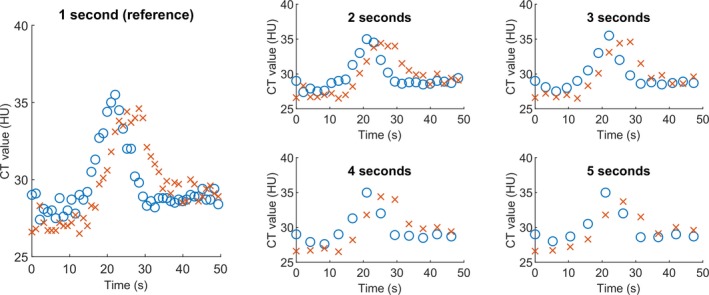
Examples of time‐attenuation curves of grey matter, illustrating the effect of reducing the acquisition interval on the attenuation curve. The blue circles illustrate an example in which the shape of the TAC is preserved with longer acquisition intervals, whereas the red crosses show a TAC which is slightly shifted in time and in which the shape is altered by the longer acquisition intervals. [Color figure can be viewed at http://wileyonlinelibrary.com]

2.2. Preprocessing

We corrected for motion by 3D rigid registration on the skull, which was done using the registration software package Elastix.17 For the bSVD and NLR methods, the CTP images were filtered with a bilateral filter, explained in detail by Bennink et al.14 A target standard deviation of the noise of 0.75 Hounsfield units was used for the filter. As for the commercial method, the CTP scans were filtered using proprietary methods which are included in the Philips ISP software.

2.3. Perfusion analysis

Tissue TAC can be regarded as convolutions of the arterial input function (AIF) with a tissue‐specific impulse response function (IRF). The shape of the IRF is determined by the different perfusion parameters (i.e., cerebral blood flow (CBF), cerebral blood volume (CBV), and mean transit time (MTT) and tracer delay). CTP analysis is a so‐called inverse problem, since the IRF has to be derived from the measured TAC and AIF:

$$TAC\left(t\right)=IRF\left(t\right)\ast AIF\left(t\right).$$ (1)

2.3.1. Non‐linear regression deconvolution

The NLR method is a non‐linear model‐based approach to solve this inverse problem. An initial guess of a block‐shaped IRF is used for the convolution, after which a residual error $\epsilon \left(t\right)$ is calculated between the estimated TAC and the measured TAC:

$$TA{C}_{\mathit{meas}}\left(t\right)=IR{F}_{\mathit{est}}\left(t\right)\ast AIF\left(t\right)+\epsilon \left(t\right).$$ (2)

Non‐linear regression is then used to iteratively update the IRF estimate to minimize the residual error. From the estimated IRF, the perfusion parameters can be calculated as shown in the article by Bennink et al.14

2.3.2. (Block‐circulant) singular value decomposition deconvolution

The convolution described in Eq. (2), can be written as a matrix operation: $b=Ax+\epsilon$, in which b is the $\mathit{TAC}$and A is a matrix containing circular shifted versions of the AIF. Vector $x$is the IRF and vector $\epsilon$ is the residual error. To get an estimate for $x$, matrix $A$ has to be inverted. In both the commercial method and in bSVD, singular value decomposition is used to find the inverse of $A$. In our bSVD implementation, noise is suppressed in the resulting IRF by removing the least significant eigenvectors until $x$ has an oscillation index below a certain threshold. In this study, acquisition interval specific oscillation indexes were used (1 s: 0.035, 2 s: 0.095, 3 s: 0.17, 4 s: 0.20, 5 s: 0.32). These values were determined by calculating the Pearson correlation between the input and observed MTT values at different oscillation indexes in simulated artificial data. For this purpose, an updated version of the anthropomorphic phantom by Riordan et al.18 was used (correlation coefficients are shown in Fig. S1). The CBF is estimated from the maximum value of vector $x$ and the CBV by calculating the ratio between the $AIF\left(t\right)$ and $TAC\left(t\right)$. The MTT is calculated from $MTT=CBV/CBF$. The ‘time insensitive’ method used in ISP (Brain Perfusion), which was used in this study, is based on bSVD.

2.3.3. Selection AIF and venous output function

In ISP, the TAC with the largest attenuation enhancement for the AIF and venous output function were automatically selected on the 1 s reference CTP image. The location of the AIF and venous output function was stored for each patient and used for all acquisition intervals, and also for the bSVD and NLR methods.

2.4. Summary maps

A summary map uses the quantitative perfusion parameters (CBF, CBV, and MTT) to estimate the infarct core, i.e., irreversible damaged brain tissue, and the penumbra, which reflects a conceptual area that may still be salvaged if recanalization of the occluded vessel is achieved in time. For the generation of the summary maps CBV and the relative MTT (rMTT) was used. The rMTT is calculated by dividing the MTT values in the ipsilateral hemisphere by the MTT value of the contralateral hemisphere. Different thresholds for the determination of infarct core and penumbra were used across the different perfusion analysis methods (Table 1).

Table 1.

The used thresholds for the calculation of the core and penumbra volumes for the different perfusion analysis methods

	Core	Penumbra
bSVD	CBV < 0.80 (ml/100g)	CBV > 0.80 (ml/100g) & rMTT > 1.30
ISP	CBV < 1.70 (ml/100g)	CBV > 1.70 (ml/100g) & rMTT > 1.85
NLR	CBV < 0.90 (ml/100g)	CBV > 0.90 (ml/100g) & rMTT > 1.35

bSVD, block‐circulant singular value decomposition; NLR, non‐linear regression; CBV, cerebral blood volume; rMTT, relative MTT.

The thresholds were calculated by maximizing the Dice overlap coefficient19 between the estimated infarct core and penumbra on the one hand, and the known volumes for those regions in the updated anthropomorphic digital phantom18 sampled at 1 s acquisition interval, on the other hand.

2.5. Image analysis

For the analysis of the CTP data, two identical circular ROIs were drawn in each hemisphere: one in the GM and one in the white matter (WM). The position and size of the ROIs was the same for the 25 datasets. These ROIs were used to calculate the average perfusion parameters (CBV, CBF, and MTT) for the patient group. The color scaling of the perfusion maps was scaled such that the mean perfusion value had the same color‐coding as the mean perfusion in the 1 s reference. In addition, the volumes of the infarct core and penumbra were measured.

2.6. Statistical analysis

The CBF, CBV, and MTT values, and the core and penumbra volumes across the different acquisition intervals were compared to the 1 s acquisition interval (reference) dataset. Differences were evaluated with the Wilcoxon signed rank test. The significance level was set to 0.05. Statistical analysis was performed in MATLAB (MATLAB R2015b).

3. Results

3.1. Quantitative perfusion values

Grey matter average perfusion values (CBF, CBV, and MTT) for the different acquisition intervals are shown in Fig. 2. The CBF, CBV, and MTT values that were significantly different from the reference standard are marked with an asterisk. ISP showed that the CBV estimates were rather constant, except for the acquisition interval of 4 s. For bSVD, CBV estimates did not show significant differences at all acquisition intervals. CBF and MTT value generated by bSVD and ISP were significantly different from the reference standard at every acquisition interval, whereas NLR did not show any significant difference in comparison to the 1 s reference.

Figure 2.

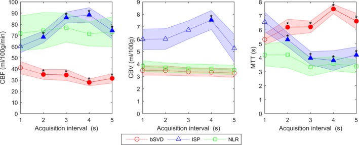
Mean perfusion parameters with 95% confidence interval for grey matter for bSVD, ISP, and NLR. The values that are significantly different from the 1 s acquisition interval (reference) are filled and marked with an asterisk. [Color figure can be viewed at http://wileyonlinelibrary.com]

In Fig. 3, the mean CBF, CBV, and MTT values of the WM are shown. The observed trends in the WM were similar to those of the GM. The CBF, CBV, and MTT values that were significantly different from the reference standard are marked with an asterisk. The perfusion analysis methods showed constant CBV values, except for ISP, for which the values at the 3 and 4 s intervals differed significantly from the reference standard. bSVD and ISP showed CBF and MTT values that were significantly different from the reference standard, whereas NLR showed no significant differences.

Figure 3.

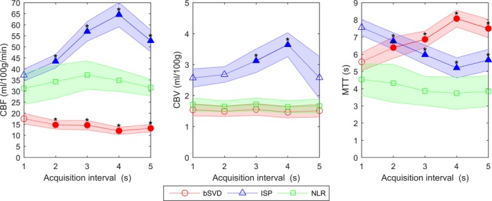
Mean perfusion parameters with 95% confidence interval for white matter for bSVD, ISP and NLR. The values that are significantly different from the 1 s acquisition interval (reference) are filled and marked with an asterisk. [Color figure can be viewed at http://wileyonlinelibrary.com]

3.2. Perfusion maps

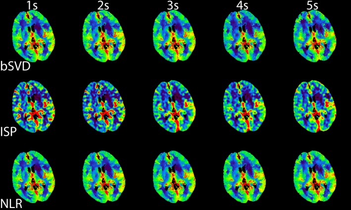
The trends observed in Figs. 2 and 3 can be used for calibrating the color‐coding range of the perfusion maps. To illustrate this for one patient, we have generated CBF maps, which are displayed in Fig. 4. These calibrated CBF maps are able to distinguish between areas of healthy and infarcted tissue up to 5 s. Hardly any differences between the CBF maps for the three CTP analysis were observed. Similarly, we generated calibrated CBV maps, which are shown in Fig. 5. The CBV maps were quite similar across the different acquisition intervals. The generated MTT maps are shown in Fig. 6. Compared to the reference standard, MTT maps generated with bSVD were relatively noisy for the 4 and 5 s acquisition intervals, whereas ISP and NLR maps are more in agreement with the reference standard.

Figure 4.

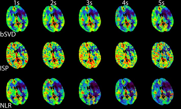
An example of calibrated CBF maps generated using bSVD, ISP, and NLR as a function of acquisition interval. [Color figure can be viewed at http://wileyonlinelibrary.com]

Figure 5.

An example of calibrated CBV maps generated using bSVD, ISP, and NLR as a function of acquisition interval. [Color figure can be viewed at http://wileyonlinelibrary.com]

Figure 6.

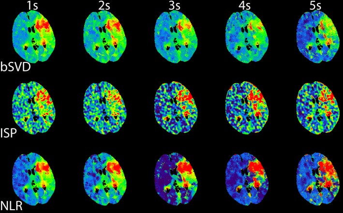
An example of calibrated MTT maps generated using bSVD, ISP, and NLR as a function of acquisition interval. [Color figure can be viewed at http://wileyonlinelibrary.com]

3.3. Summary maps

The summary maps were generated for every acquisition interval. The summary maps for one patient are shown in Fig. 7. Visually, the summary maps generated with bSVD were rather similar to the reference summary map. Summary maps generated with ISP were similar up to an acquisition interval of 4 s, but the 5 s acquisition interval summary map had a significant increase in core volume (red) than the reference standard. Still, the 5 s acquisition interval summary map looks quite similar to the reference standard. Summary maps generated with NLR were fairly constant. In the supplementary materials, summary maps from two other patients show similar differences (Figs. S2 and S3).

Figure 7.

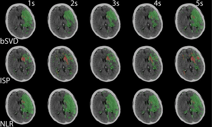
Summary maps of bSVD, ISP, and NLR as a function of acquisition interval. The infarct core is labeled red, the penumbra labeled green. This is the same patient as shown in Figs. 4, 5, 6. [Color figure can be viewed at http://wileyonlinelibrary.com]

Average core and penumbra volumes generated by the three CTP analysis methods are shown in Fig. 8. Core volumes generated by bSVD and NLR show a monotonic significant increase with increased acquisition interval. Core volumes generated by ISP shows a monotonic decrease in volume, with a large significant increase for the 5 s volume. The core volume was significantly different from the reference standard at 3, 4, and 5 s intervals. The penumbra volumes generated by bSVD and NLR did not show any significant differences, except for the penumbra volume generated with bSVD on the 5 s interval. Penumbra volumes generated with ISP were all significantly larger than the reference standard.

Figure 8.

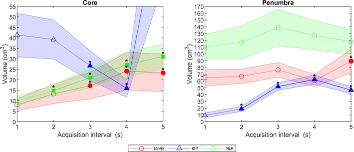
Mean volumes (cm³) with 95% confidence interval of the infarct core and the penumbra. If the volume was significantly different from the reference standard it is filled and marked with an asterisk. The 5 s ISP core volume was over 100 cm³ and therefore not included in the figure. [Color figure can be viewed at http://wileyonlinelibrary.com]

4. Discussion

In this study, the response of three perfusion analysis methods to different acquisition intervals was investigated by analyzing CTP data from 25 patients with ischemic stroke. ISP overestimated the CBF and CBV and underestimated MTT as compared to the 1 s reference standard in the grey and WM (Figs. 2 and 3). The 5 s dataset, however, deviated from this trend. This trend was already observed by Wintermark et al. 9 When using a 40 ml iodinated contrast bolus, Wintermark et al. did not observe significant differences up to an acquisition interval of 3 s, whereas in our dataset we observed significant differences at 2 s, except for the CBV values. There are two main causes of the observed differences. Firstly, Wintermark et al. acquired at 80 kVp and 120 mAs every 0.5 s, whereas we acquired CTP data at 80 kVp and 75 mAs every second. As a consequence, our images are significantly noisier. Secondly, Wintermark et al. used the so‐called ‘arrival time sensitive’ algorithm, whereas we used the newer ‘arrival time insensitive’ algorithm, which might potentially lead to observed differences.

The observed differences between bSVD and ISP were caused by differences in the used oscillation index, filtering and postprocessing. As hypothesized, perfusion values generated with NLR were not significantly different across the different acquisition intervals indicating that NLR estimates perfusion parameters in a more robust manner. This can probably be explained by the fact that most TACs have long enough MTTs maintaining the fit of the curve. As a result, NLR generated accurate estimates even with prolonging acquisition intervals. We did observe a large variance in the CBF and MTT values of NLR compared to the other methods, which can be attributed to the fact that we saw large interpatient differences, but not large differences with increasing acquisition intervals within a patient. In addition, the large variance is due to regularization of the TACs, which makes the estimates of NLR more realistic, but this results in an increase in variance of the CBF. bSVD and ISP generated significantly different CBF and MTT values for all acquisition intervals compared to the reference standard. However, because a similar acquisition interval‐dependent trend was observed in both the grey and WM, the perfusion maps could be appropriately generated by calibrating the color‐coding based on the observed values (Figs. 4, 5, 6). This suggests that the over‐ or underestimation of the perfusion variables by the CTP analysis methods is a systemic bias dependent on acquisition interval and that the distinction between healthy and infarcted tissue can still be made for acquisition intervals of up to 5 s. The approach of calibrating the color‐coding range, however, is not validated on a separate independent dataset and thus needs further evaluation.

Block‐circulant singular value decomposition and NLR generated infarct core volumes (Fig. 8), which increased with increasing acquisition intervals is mainly due to an increase in remote voxels misclassified as core due to noise. This issue can possibly be solved by introducing a postprocessing filter step, which removes these spurious pixels and subsequently reduces the infarct core volumes for prolonged acquisition intervals. For ISP, a decrease in core volume was observed with increasing interval, mainly due to the overall increase of the CBV values and could possibly be solved by scaling the core thresholds. ISP generated significantly higher penumbra volumes with increasing acquisition intervals, which can be attributed to the number of remote pixels misclassified as penumbra. For bSVD and NLR, only a minor change in penumbra volumes with increasing acquisition interval was shown, which can be explained by the slight increase in noise in the summary maps due to noise. 

Even though changes in infarct core and penumbra volumes are observed, the summary maps (Fig. 7) show that with acquisition intervals of at least 4 (ISP) and 5 (bSVD and NLR) seconds it is still feasible to distinguish between infarcted and healthy tissue.

This study has several limitations. Firstly, we did not have any validation of the true infarct core and penumbra volumes in the patient data. However, as we were only interested in the differences that arise from using different acquisition intervals, we do not think that this limitation impacts our conclusions. Still, comparison with a reference standard such as DWI MRI would be needed in future studies before these methods can be safely used in stroke care. Secondly, to create CTP datasets with increasing acquisition intervals, we deleted images from a 1 s reference dataset. It would have been ideal if we could have scanned every patient with the five different acquisition intervals. However, this approach would not be ethical and we feel that our used methods simulate repeated scanning on different acquisition intervals appropriately. Thirdly, there are no standardized thresholds available for bSVD and NLR to calculate infarct volumes. To quantify any bias in volume due to the longer acquisition intervals, we decided to calculate thresholds optimal for all methods for this dataset. The used core and penumbra volume thresholds are not verified for a large variety of patient groups, and there is no justification for the method used to generate the volumes. The purpose of the generation of the volumes was mainly to illustrate that infarct volumes are reliable with longer acquisition intervals. Lastly, to evaluate Jog Mode we looked at acquisition intervals of up to 5 s, but we did not include the movement of the table, which causes a time shift in the TACs of the top and bottom half of the brain. However, since the used methods are insensitive to bolus arrival time by design, we feel that this time shift has had little effect on the generated perfusion parameters.

5. Conclusion

Altering the acquisition interval may introduce a bias in the perfusion parameters. However, calibration of the visualization of the perfusion maps with increasing acquisition intervals allowed distinction between healthy and infarcted tissue. Even though infarct volumes based on relative rMTT can be influenced by the acquisition interval, visual inspection of the summary maps indicated minor differences between the reference standard and acquisition intervals up to 4 (ISP) and 5 s (bSVD and NLR). Taken together, dependent on the used CTP analysis method, axial coverage can be increased by prolonging the acquisition interval up to 5 s without affecting the generation of accurate perfusion parameters and infarct volumes.

Supporting information

Fig. S1. Pearson correlation coefficients of MTT values for non‐commercial bSVD analysis at different oscillation indexes. The maximum correlation was with oscillation index of 0.035, 0.095, 0.170, 0.200 and 0.320 for the 1, 2, 3, 4, and 5 s acquisition intervals, respectively.

Fig. S2. Summary maps of bSVD, ISP, and NLR as a function of acquisition interval. The infarct core is labeled red, the penumbra labeled green. For bSVD and NLR, the maps appear constant. For ISP, the penumbra volume is quite constant with increasing interval, whereas a core volume is hardly visible, except for the large increase at 5 s.

Fig. S3. Summary maps of bSVD, ISP, and NLR as a function of acquisition interval. The infarct core is labeled red, the penumbra labeled green. This was one of the best examples for bSVD and NLR, in which hardly any differences are observed compared to the 1 s reference, whereas ISP shows the decrease in core volume with increasing interval.

References

- 1. Lövblad K‐O, Baird AE. Computed tomography in acute ischemic stroke. Neuroradiology. 2010;52:175–87. [DOI] [PubMed] [Google Scholar]
- 2. Wintermark M, Luby M, Bornstein NM, et al. International survey of acute stroke imaging used to make revascularization treatment decisions. Int J Stroke. 2017;10:759–762. [DOI] [PMC free article] [PubMed] [Google Scholar]
- 3. de Lucas EM, Sánchez E, Gutiérrez A, et al. CT protocol for acute stroke: tips and tricks for general radiologists. Radiographics. 2008;28:1673–1687. [DOI] [PubMed] [Google Scholar]
- 4. Albers GW, Marks MP, Kemp S, et al. Thrombectomy for stroke at 6 to 16 hours with selection by perfusion imaging. N Engl J Med. 2018;378:708–718. [DOI] [PMC free article] [PubMed] [Google Scholar]
- 5. Nogueira RG, Jadhav AP, Haussen DC, et al. Thrombectomy 6 to 24 hours after stroke with a mismatch between deficit and infarct. N Engl J Med. 2018;378:11–21. [DOI] [PubMed] [Google Scholar]
- 6. Emmer BJ, Rijkee M, Niesten JM, et al. Whole brain CT perfusion in acute anterior circulation ischemia: coverage size matters. Neuroradiology. 2014;56:1121–1126. [DOI] [PubMed] [Google Scholar]
- 7. Biesbroek JM, Niesten JM, Dankbaar JW, et al. Diagnostic accuracy of CT perfusion imaging for detecting acute ischemic stroke: a systematic review and meta‐analysis. Cerebrovasc Dis. 2013;35:493–501. [DOI] [PubMed] [Google Scholar]
- 8. Wintermark M, Fischbein NJ, Smith WS, et al. Accuracy of dynamic perfusion CT with deconvolution in detecting acute hemispheric stroke. Am J Neuroradiol. 2005;26:104–112. [PMC free article] [PubMed] [Google Scholar]
- 9. Wintermark M, Smith WS, Ko NU, et al. Dynamic perfusion CT: Optimizing the temporal resolution and contrast volume for calculation of perfusion CT parameters in stroke patients. Am J Neuroradiol. 2004;25:720–729. [PMC free article] [PubMed] [Google Scholar]
- 10. Kämena A, Streitparth F, Grieser C, et al. Dynamic perfusion CT: Optimizing the temporal resolution for the calculation of perfusion CT parameters in stroke patients. Eur J Radiol. 2007;64:111–118. [DOI] [PubMed] [Google Scholar]
- 11. Wiesmann M, Berg S, Bohner G, et al. Dose reduction in dynamic perfusion CT of the brain: effects of the scan frequency on measurements of cerebral blood flow, cerebral blood volume, and mean transit time. Eur Radiol. 2008;18:2967–2974. [DOI] [PubMed] [Google Scholar]
- 12. Abels B, Klotz E, Tomandl BF, et al. CT perfusion in acute ischemic stroke: A comparison of 2‐second and 1‐second temporal resolution. Am J Neuroradiol. 2011;32:1632–1639. [DOI] [PMC free article] [PubMed] [Google Scholar]
- 13. Cao G, Chen W, Sun H, et al. Whole‐brain CT perfusion imaging using increased sampling intervals: a pilot study. Exp Ther Med. 2017;14:2643–2649. [DOI] [PMC free article] [PubMed] [Google Scholar]
- 14. Bennink E, Oosterbroek J, Kudo K, et al. Fast nonlinear regression method for CT brain perfusion analysis. J Med Imaging. 2016;3:026003. [DOI] [PMC free article] [PubMed] [Google Scholar]
- 15. Wu O, Østergaard L, Weisskoff RM, et al. Tracer arrival timing‐insensitive technique for estimating flow in MR perfusion‐weighted imaging using singular value decomposition with a block‐circulant deconvolution matrix. Magn Reson Med. 2003;50:164–174. [DOI] [PubMed] [Google Scholar]
- 16. Niesten JM, Van Der Schaaf IC, Riordan AJ, et al. Radiation dose reduction in cerebral CT perfusion imaging using iterative reconstruction. Eur Radiol. 2014;24:484–493. [DOI] [PubMed] [Google Scholar]
- 17. Klein S, Staring M, Murphy K, Viergever Ma, Pluim J. elastix: a toolbox for intensity‐based medical image registration. IEEE Trans Med Imaging. 2010;29:196–205. [DOI] [PubMed] [Google Scholar]
- 18. Riordan AJ, Prokop M, Viergever MA, et al. Validation of CT brain perfusion methods using a realistic dynamic head phantom. Med Phys. 2011;38:3212–3221. [DOI] [PubMed] [Google Scholar]
- 19. Dice LR. Measures of the amount of ecologic association between species. Ecology. 1945;26:297–302. [Google Scholar]
Associated Data
This section collects any data citations, data availability statements, or supplementary materials included in this article.
Supplementary Materials