Automated Segmentation of the Left and Right Ventricles in 4D Cardiac SPAMM Images

Abstract

In this paper we describe a completely automated volume-based method for the segmentation of the left and right ventricles in 4D tagged MR (SPAMM) images for quantitative cardiac analysis. We correct the background intensity variation in each volume caused by surface coils using a new scale-based fuzzy connectedness procedure. We apply 3D grayscale opening to the corrected data to create volumes containing only the blood filled regions. We threshold the volumes by minimizing region variance or by an adaptive statistical thresholding method. We isolate the ventricular blood filled regions using a novel approach based on spatial and temporal shape similarity. We use these regions to define the endocardium contours and use them to initialize an active contour that locates the epicardium through the gradient vector flow of an edgemap of a grayscale-closed image. Both quantitative and qualitative results on normal and diseased patients are presented.

1. Introduction

Cardiovascular disease is the leading cause of death in many developed countries. To reduce morbidity, quantifying the motion of the heart is valuable for understanding normal and abnormal physiology and for patient diagnosis. SPAMM [1,2], is a promising non-invasive technique for measuring the shape and motion of the heart. Parallel sheets of tissue are magnetically tagged at end-diastole and they appear as dark lines when imaged in the direction normal to the sheets. This paper presents a completely automated method to find the epicardium and endocardium contours in tagged MR images. The endocardium segmentation is challenging because the tag lines obscure these contours and the images tend to have low contrast between the blood and the myocardium and because the intensities of the tissue change as the tags fade and new blood enters the heart. Epicardium segmentation is challenging because the boundary is occluded by adjacent structures such as the liver or a layer of fat.

Tracking the motion of the tag sheets provides 3D information about the motion of the myocardium and there has been significant research [3–8] into methods for automating tag sheet tracking. These methods are more accurate [3,4] when the epicardium and endocardium contours are provided because the contours restrict the search space for tag sheets to the myocardium. Methods that do not use the epicardium and endocardium contours have limited applicability in the thin walled structures such as the RV (right ventricle) where there is a sparsity of tags to track. It has been shown[9] that if the epicardium and endocardium contours could be segmented then measuring the 3D shape deformation in thin walled structures such as the RV becomes possible through finite element analysis. It has also been shown [10–12] that endocardium and epicardium contours can be used in conjunction with tag sheet tracking to determine a low dimensional, clinically relevant description of the motion of the LV (left ventricle). Moreover, the contours help identify and track key anatomical features useful for the inter-subject comparison of strain fields recovered from these tag tracking. The contours can also be used directly to measure ejection fraction, and wall thickening. Several researchers have developed methods for locating the contours of the heart in tagged MR images. The system proposed by Guttman et al. [13] was able to delineate the contours of the LV on radially tagged SA (short axis) slices using a dynamic programming method based on a minimum cost algorithm after the user indicated the center of the LV cavity and the region of interest. Goutsias [14] proposed a watershed segmentation method to locate the contours of the LV in SA images. While we have not directly used these techniques due to their inapplicability to our problem, these papers have influenced our work. Our method does not require any user interaction to segment the left and right ventricles. Some of these systems appear to require dark blood. Procedures such as “black blood” imaging add complexity and some time to the image acquisition procedure. Our method does not require this extra step. Another advantage of our method is that it requires only raw SPAMM data acquisition, not CSPAMM data acquisition which can substantially increase acquisition time which is problematic for the patient with cardiac disease, not accustomed to long periods of continual breath holding.

We have found that 80% or 4 of the 5 hours required to analyze tagged SPAMM data sets involves the outlining the contours of the ventricles. We present a method that directly addresses this most significant portion of the analysis time by segmenting the endocardium and epicardium contours without requiring user input. In section 2, we describe how we remove background intensity variation in each volume to prepare the volumes for segmentation. In section 3 and 4 we describe how we locate the heart and segment the endocardium and epicardium in the corrected volumes. We provide qualitative and quantitative results in section 5 and our conclusions in section 6.

2. Volumetric Intensity Correction

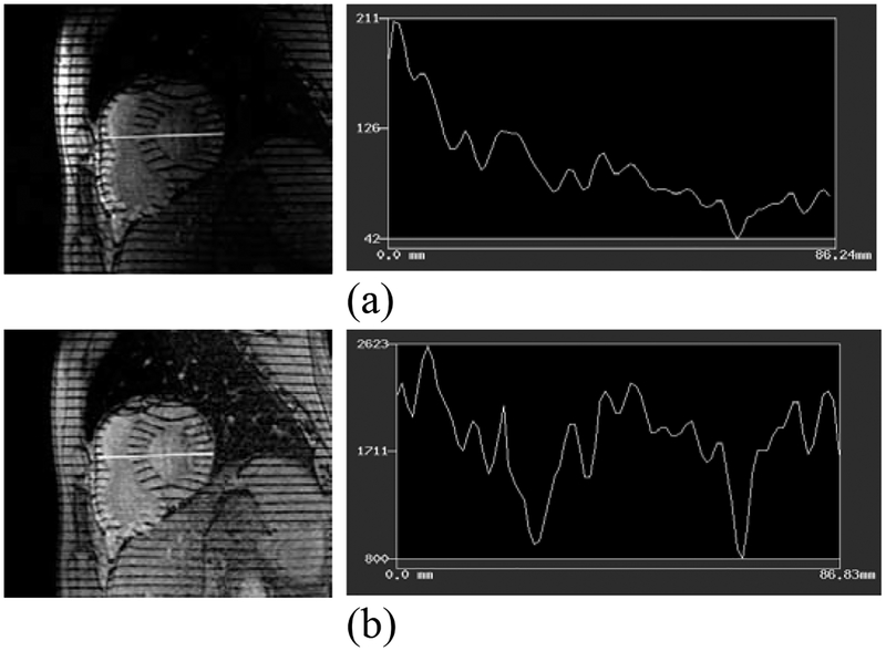
Tagged images are acquired mostly with one and sometimes with two surface coils. While the coils increase image contrast, they can also cause the same tissue to have different intensities depending on its location in the image. We use a new scale-based correction procedure to correct the background intensity variation throughout each volume. A variety of techniques have been employed to correct background intensity variation in MRI, few meet the following requirements that make them clinically useful: (1) no user input is needed on a per volume basis (2) the method is pulse sequence and surface coil independent (3) intensity distributions for tissue classes need not be known. Details on this method, including its performance on non-cardiac images can be found in [15]. We present an overview of the method and a modification that works well for all of the subjects that we have processed. We have found empirically that iterating the steps below 10 times works well for all subjects. Fig. 1 shows a sample slice from a corrected volume.

Fig. 1.

1D intensity profiles are plotted for the white lines shown in the images: (a) before correction (b) after correction. Intensity through the heart is much more uniform after correction; the two prominent intensity valleys are caused from the sampling line skimming two tags which remain dark after correction

1. 1. Given a volume $f(\overline{x})$ , define the foreground volume as:

$$f{}_{\mathit{\text{foreground}}}(\overline{x})=\{\begin{array}{ll}1\hfill & f(\overline{x})>\mathit{\text{mean}}(f(\overline{x}))\hfill \\ 0\hfill & \mathit{\text{otherwise}}\hfill \end{array}$$

1. 2. Compute the scale volume $f_{\mathit{\text{scale}}}(\overline{x})$ for the pixels where $f_{\mathit{\text{foreground }}}(\overline{x})=1$. Scale at a pixel is defined as the radius of the largest ball centered at the pixel for which a pixel intensity homogeneity measure [15] is preserved.

2. 3. Let S_max be the maximum value in $f_{\mathit{\text{scale}}}(\overline{x})$ and let the set PixelsOfSmax be the set of all pixels in the scale image that have a scale of S_max. Compute the mean μ and standard deviation σ of the intensities in $f(\overline{x})$ for the pixels of PixelsOfSmax. Let the set objectPixels be the set of pixels in the volume that have intensities in the interval [μ – ασ, μ + βσ]. For tagged MR, the objects we are most interested in correcting are the bright objects (the myocardium and blood regions) and we find empirically that setting α= 1.0 and β= 5.0 works well for all subjects.

3. 4. To estimate the background intensity variation, a 2^nd order polynomial $\beta (\overline{x})$ is fitted to the normalized intensities in objectPixels by minimizing

$$\sum _{v\in \mathit{\text{objectPixels}}}{\left[\beta (v)-f(v)/{\mu }_{\mathit{\text{objectPixels}}}\right]}^2$$

1. 5. In MRI, background intensity variation is typically modeled as multiplicative noise, therefore image is corrected by replacing $f(\overline{x})\text{ with}\raisebox{1ex}{$f(\overline{x})$}\!\left/ \!\raisebox{-1ex}{$\beta (\overline{x})$}\right.$.

3. Endocardium Segmentation

The endocardium contours are the boundaries between the blood filled ventricular cavities and the myocardium. To locate these boundaries reliably we look for strong image features that are present for every subject. Since we are not using “black blood” imaging, the blood appears bright and we leverage this fact to accurately locate the salient blood filled cavities of the LV and RV and the inflow and outflow tracts of the RV. In all our images from the second time (second volume) the motion of the blood has washed out the tags. We begin our endocardium segmentation in this volume by applying a 3D grayscale morphological opening operation. Let the given volume be $f(\overline{x})$ where $\overline{x}$ is an element of the domain of $f:\overline{x}\in D_f$ and let the structuring element be $b(\overline{x})$ where $\overline{x}\in D_b$. Then the gray-scale opening of f by b is written as $f°b=(f-b)\oplus b$ where f − b is the gray-scale erosion of f by b defined in eqn (1a) and f Å b is the gray-scale dilation of f by b defined in eqn (1b)

$$\begin{gathered} (a)(f-b)(\overline{s})=\text{min}\left\{f(\overline{s}+\overline{x})-b(\overline{x})|\overline{s}+\overline{x}\in D{}_f;\overline{x}\in D_b\right\} \\ (b)(f\oplus b)(\overline{s})=\text{max}\left\{f(\overline{s}-\overline{x})+b(\overline{x})|\overline{s}-\overline{x}\in D{}_f;\overline{x}\in D_b\right\} \end{gathered}$$ (1)

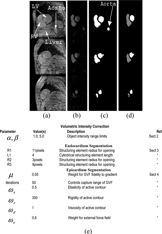
The intensity value at a pixel $\overline{x}$ in the opened volume is the maximum of the minimum values in the pixels covered by the structuring element when centered at $\overline{x}$ We use a binary 3D cylinder shaped structuring element whose radius, R1, is 1.5 times the tag separation width and whose length L1 spans 4 image planes. We have found that this structuring element gives the best initial segmentation of the blood filled regions of the images. The radius is sufficient to cover at least 2 tags; therefore even if noise has corrupted one tag, the other tag covered by the structuring element will enable the opening result to reflect the presence of tags. Fig. 2b shows sample slices from the opening of a volume at time 2.

Fig. 2.

Steps to find the endocardium (a) 3 slices from original volume (b) grayscale opened volume (c) thresholded volume (d) pruned volume using shape similarity. Note the aorta has been pruned away. (e) Algorithm parameters

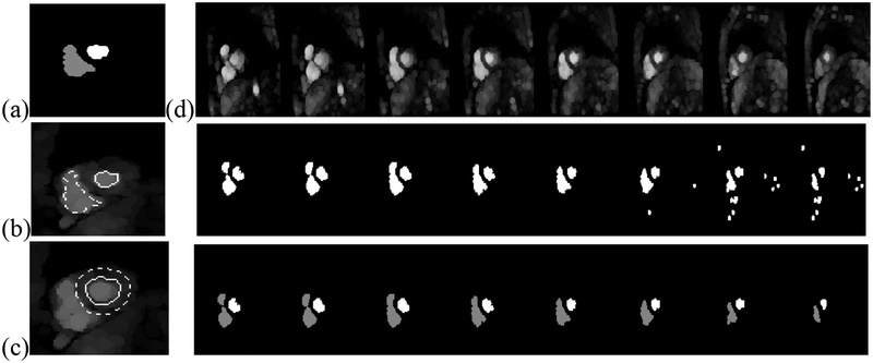
An important advantage in this cavity-locating method is that it can be applied without change in all the slices through the heart. For example the bifurcation of the right ventricle into inflow and outflow tracts can be located (see first column in Fig. 4d). In slices through the tip of the apex (not shown), a blood filled region is detected only if present. This property is important since in some subjects the apex of the LV cavity is inferior to the apex of the RV cavity, while for other subjects the reverse is true. We note that this gray-scale opening based method can detect whether there are blood filled regions are present –down to the size of the structuring element used in the opening operation. For our images this is rarely a significant limitation since the tags are closely spaced (6 pixel spacing), yielding a small-diameter structuring element.

Fig. 4.

(a) Mid ventricular regions from the previous time. Contours from these two regions are used to delineate regions on the same slice for the current time to sample blood tissue, [the regions inside the contours in (b)] and to sample the myocardium [using the region in between the contours in (c)]. In (d) the endocardium processing steps are shown for all slices for one time. First row: opened images. Second row: results from adaptive thresholding. Third row: results from shape similarity pruning

Next, we threshold the images and fill the holes with a binary morphological closing operation. To select the threshold in this initial time, we use the threshold that minimizes the variance of the pixels grouped into the foreground object. The results of thresholding these images are shown in Fig. 2c.

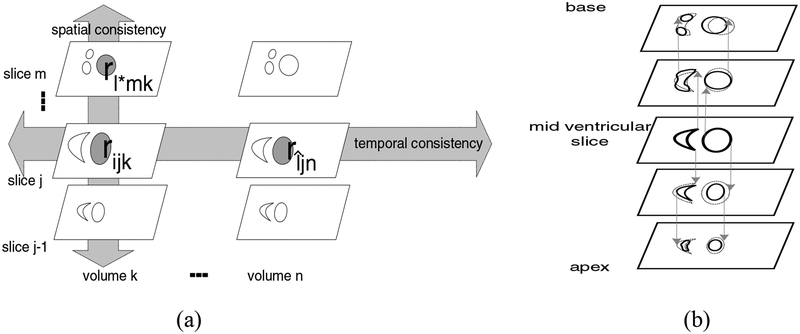
To identify which of these binary regions are from the ventricles, we first find the binary regions corresponding to the LV and RV on a mid-ventricular slice. To identify a mid ventricular slice, as well as the pair of regions forming the LV and RV cavities on that slice, we find the most spatially consistent pair of regions. We describe this measure formally with the following definitions and the accompanying drawing (Fig 3a).

Fig. 3.

(a) For a given region r_ijk, the regions on slice m in volume k are searched to find the most spatially similar region$r_{l^{*}mk}$. The regions on slice j in volume n are searched to find the most temporally similar region, r_îjn (b) Orthographic projection to form the LV and RV cavities

We are given a short axis dataset consisting of a set V of N volumes: V = {v_k}where k ∈[1..N] Each volume consists of a set S of M slices: S = {s_j} where j ∈[1..M]. After thresholding a morphologically opened volume, the j^th slice on the k^th frame consists of a set R of B(j,k) regions R = {r_i } where i ∈[1..B(j,k)].

We define the similarity in eqn 2., as in [16]. The similarity between region r_ijk (the i^th region on the j^th slice of the k^th volume) and the region r_ljm (the l^th region on the m^th slice of the n^th volume) is

$$Sim\left(r_{ijk},r_{lmn}\right)=\frac{\mathit{\text{area}}\left(\cap \left\{r_{ijk},r_{lmn}\right\}\right)}{\mathit{\text{area}}\left(\cup \left\{r_{ijk},r_{lmn}\right\}\right)}$$ (2)

the area of their intersection divided by the area of their union. For a given region r_ijk the most similar region $r_{l^{*}mk}$ spatially and the most similar region r_îjn temporally are defined as:

$$r_{l^{*}mk}=\underset{l\in B(m,k),m\ne j}{\text{arg}\text{max}}Sim\left(r_{ijk},r_{lmk}\right)r_{ijn}=\underset{l\in B(j,n),n\ne k}{\text{arg}\text{max}}Sim\left(r_{ijk},r_{ljn}\right)$$ (3)

To find the LV or the RV on the mid ventricular slice we define the spatial shape consistency and temporal shape consistency of a region r_ijk as:

$$ssc\left(r_{ijk}\right)=\sum _{m=1,m\ne j}^{M}Sim\left(r_{ijk},r_{l^{*}mk}\right)tsc\left(r_{ijk}\right)=\sum _{n=1,n\ne k}^{N}Sim\left(r_{ijk},r_{\widehat{l}jn}\right)$$ (4)

To find the pair of LV and RV regions on the mid ventricular slice we define the spatially consistent region pair $\left(r_{\tilde{i}\tilde{j}k},r_{\tilde{l}jk}\right)$ as:

$$\left(r_{\tilde{i}\tilde{j}k},r_{\tilde{l}\tilde{j}k}\right)=\underset{i,l\in B\left(j,k\right),i\ne l}{\underset{j\in \left[\mathrm{1..}M\right]}{\text{arg}\text{max}}}\left\{ssc\left(r_{ijk}\right)+\text{ssc}\left(r_{ljk}\right)\right\}$$ (5)

and we define the most spatially and temporally consistent region pair as the pair $\left(r_{\tilde{i}\tilde{j}k},r_{\tilde{l}jk}\right)$ of regions whose spatial and temporal shape consistency values are maximal:

$$\left(r_{\tilde{i}\tilde{j}\tilde{k}},r_{\tilde{l}\tilde{j}k}\right)=\underset{\underset{\underset{i,l\in B\left(j,k\right),i\ne l}{k\in \left[\mathrm{1..}N\right]}}{j\in \left[\mathrm{1..}M\right]}}{\text{argmax}}\left\{ssc\left(r_{ijk}\right)+tsc\left(r_{ijk}\right)+ssc\left(r_{jk}\right)+tsc\left(r_{jk}\right)\right\}$$ (6)

The RV bifurcates at the base of the heart into inflow and outflow tracts and has a tapered lobe below the base, while the cavity of the LV resembles a prolate spheroid cropped at the top. Consequently, in the thresholded images, three regions appear in the base (RV inflow and outflow tracts and the LV cavity), two relatively large regions appear in the mid-ventricular images and two small regions appear near the apex. Because of these characteristics, the most spatially consistent region pair in the thresholded images is the pair of regions from the mid ventricular slice from the LV and RV. The LV and RV regions near the apex are too small to be the most spatially consistent pair and the inflow and outflow tracks at the base prevent the base slices from being the slice containing the most consistent pair. In addition the regions from the aorta are not part of the most spatially consistent pair because they receive low spatial shape consistency scores because the aorta does not run throughout the whole short axis volume and because the aorta is typically not oriented perpendicular to the short axis image planes. Regions from the blurring of tags due to motion artifacts, which can appear on an individual slice, are also not in the most spatially consistent pair because they do not extend throughout the short axis volume.

The mid-ventricular slice is the slice with the pair of most spatially consistent regions. We attach the regions in the superior and inferior slices that have sufficient intersection with these pairs. We determine which regions overlap through orthographic projection. To form the base volume of the cavities, we project the regions on the current slice (initially the mid ventricular slice) up to the next slice orthographically (see Fig 3b). The regions that overlap are connected to the regions from the previous slice. To form the apical volume of the cavities, we project the regions on the current slice (initially the mid ventricular slice) down to the next slice orthographically and the regions that overlap are connected to the regions from the previous slice. The boundaries of the cavities define the boundary between the blood and the myocardium and thereby yield the endocardium.

For subsequent times we begin the processing by opening the volumes with the 3D structuring element described above. To choose a threshold for the opened images, we use the segmentation map from the prior time. As shown in Fig. 4 (a)-(c), the endocardium regions found in the previous time are propagated onto the grayscale-opened image of the current time.

The ventricular cavity regions on the mid-ventricular slice (Fig 4a) from the previous volume are eroded by a disk of radius 3 pixels and their boundaries are propagated to the same slice on the next volume. We estimate the mean intensity of the pixels in the blood region on the opened image by computing the mean of the intensities of the pixels in this region (Fig. 4b). To compute the mean of the intensity of the myocardium portion of the opened volume we form a ring shaped sampling region by dilating the LV endocardium region from the previous volume’s mid ventricular slice by a disk of radius, R4 of 3 pixels and a disk of radius, R3 of 9 pixels. This band is propagated to the same slice on the next volume and is located roughly in the center of the myocardium of the LV (Fig. 4c).

We identified which region was the LV from the pair of regions on the mid ventricular slice in the previous volume by noting which orthographically connected region bifurcated in the base (the RV bifurcates) or if neither has then the LV is identified as the region which has a smaller volume above the mid ventricular slice. In our datasets this provides an accurate determination of the RV and LV because the RV is typically larger than the LV and the RV volume includes the inflow and outflow tracks. Also it is important to use our knowledge of the mid ventricular slice: propagating contours from the mid ventricular slice to the same slice on the next volume works well, however if we propagated contours from a base slice to the same slice on the next volume, topological changes in the RV (see Fig. 5) can render the blood intensity sampling less accurate.

Fig. 5.

All endocardium contours (dashed) and epicardium contours (solid) over time 2 through end ES (end systole) for a particular slice near the base

The opened images from the current time are then thresholded with the mean of the mean intensities of the blood and myocardium tags: δ_thresh=(μ_blood+μ_myo)/2. We have found that this threshold selection method compares well with thresholds selected manually by selecting an intensity at a valley between peaks in the histogram of the opened image. Moreover the intensity inhomogeneity correction step described in the previous section makes the intensities of tissues within each volume more uniform and improves the results of thresholding the opened images using a threshold from the mid ventricular slice. Once we have thresholded the opened volume we compute the most spatially and temporally consistent binary region pair in the slices of each volumes processed thus far and attach the regions in the superior and inferior slices as described above. Since the base moves toward the apex, the mid-ventricular slice can change over time. By using both temporal consistency and spatial consistency we are able to update the mid-ventricular slice to be the slice that contains the pair of regions that change the least over time and throughout the imaged volume. The results for several times are shown in Fig. 5.

4. Epicardium Segmentation

We are interested in finding a contour on each slice that defines the epicardium of the heart, which is the boundary between the myocardium and the tissues that surround the heart. The epicardium is typically harder to segment than the endocardium because there is little contrast between the myocardium and surrounding tagged structures, such as the liver and the chest wall. Fat often appears as a partial ring of tissue surrounding the heart and is particularly challenging to handle since the ring is narrow. Fat is often included in the myocardium in methods that attempt to segment the endocardium in tagged MR images. Here we present an automatic method that largely overcomes this problem by expanding a physics-based deformable model known as an active contour [17] from the interior of the heart towards the exterior edge of the myocardium so that it will stop when it gets to the dark pixels between the myocardium and fat.

We fill the tags in each slice at each time with a linear structuring element whose width is equal to the tag width. In our images the structuring element is 4 pixels and the filled images are shown in Fig. 6(b). This fills in all the tags while leaving most borders intact. Next we adaptively Wiener filter the filled images to smooth the intensities of the myocardium while preserving edges. We apply less filtering where the local intensity variance is large and greater filtering where the local variance is small. Fig. 6(c) shows the result, which we will refer to as f (x, y) . The magnitude of the gradient of this image, with edges in the endocardium regions found in section 3 suppressed, is shown Fig. 6(d). We compute a gradient vector flow (GVF) [18] field (see Fig 6(e)) from ∇f to provide forces for the deformable model. The GVF field captures object boundaries from either side and consists of a 2D vector field $\overline{v}(x,y)={(u(x,y),v(x,y))}^T$that minimizes the energy in eqn 7a. The PDE (eqn 7b) that minimizes this functional is found through the calculus of variations and the equilibrium solution to this equation defines the flow field.

Fig. 6.

Epicardium segmentation steps: (a) original image (b) grayscale closing (c) adaptive Wiener filtering (d) edge map (e) gradient vector flow field (f) Segmented LV-RV epicardium (single solid line) and separate, manual RV and LV epicardium (dotted lines)

$$\begin{gathered} \text{ (a) }E(\overline{v})=\iint \mu \left(u_x^2+u_y^2+v_x^2+v_y^2\right)+\left|\nabla f{|}^2\right|\overline{v}-\nabla f{|}^2\mathit{\text{dxdy}} \\ \text{(b) }{\overline{v}}_t=\mu {\nabla }^2\overline{v}-|\nabla f{|}^2(\overline{v}-\nabla f) \\ \text{(c) }{u}_t=\frac{1}{\Delta t}\left(u_{i,\mathrm{j}}^{n+1}-u_{i,j}^n\right){\nabla }^{2}u=\frac{1}{\mathrm{\Delta }x\mathrm{\Delta }y}\left(u_{i+1,j}+u_{i,j+1}+u_{i-1,j}+u_{i,j-1}-4u_{i,j}\right) \end{gathered}$$ (7)

We favor strong fidelity of the GVF field to ∇f since there are weak edges between the heart and liver that we want to capture with the active contour. We have found that setting μ =0.05 works well to segment the epicardium. To form an initial epicardium contour for our physics-based deformable model we construct the convex hull of the RV and LV regions from the previous section. We have found that using discrete approximations shown in eqn. 7c to the partial derivatives in eqn. 7b with Δt = Δx = Δy = 1and iterating a forward Euler finite difference scheme 50 times is sufficient to extend the capture range of the initial active contour to segment the epicardium.

Our physics-based deformable active contour, X (s) , is parameterized by arc length and deforms according to Newton’s second law (eqn. 8a). To stop at weak edges we set the mass, m, of the contour to zero. The governing motion equation (eqn. 8b) is formed by defining the internal force from the stretching and bending of the semi-rigid contour and the external force from the gradient vector flow field, $\overline{v}$.

$$\begin{gathered} (a)m\frac{{\partial }^{2}X}{\partial t^2}=F_{\mathit{\text{dampening}}}(X)+F_{\mathit{\text{internal}}}(X)+F_{\mathit{\text{external}}}(X) \\ (b)\underset{-F_{\mathit{\text{dampening}}}}{\underbrace{{\omega }_d\frac{\partial X}{\partial t}}}=\underset{F_{\mathit{\text{internal}}}}{\underbrace{\frac{\partial }{\partial s}\left({\omega }_s\frac{\partial X}{\partial s}\right)+\frac{{\partial }^2}{\partial s^2}\left({\omega }_r\frac{{\partial }^{2}X}{\partial s^2}\right)}}+{\omega }_e\underset{F_{\mathit{\text{external}}}}{\underbrace{\overline{v}(X)}} \end{gathered}$$ (8)

The parameters used to control the deformable model are: elasticity ω_s =0.5, rigidity ω_r =350, viscosity ω_d =1 and external force field weight ω_e =0.6. We have found these values work well on all of our tests for both normal and diseased hearts. We approximate the derivatives with finite differences and iterate a forward Euler finite difference scheme until the contour converges. We define convergence to occur when the contour area has not changed appreciably (1 pixel area) over the last 10 iterations. In all our tests convergence occurs within 85 iterations. In Fig 7(a)-(e) we see that our approach has avoided classifying the ring of fat which appears near the top of the epicardium as myocardium. In Fig. 7(a),(c) the triangular shaped fat region which appears near the bottom left corner of the epicardium has also been excluded from the myocardium.

Fig. 7.

The expansion of an initial active contour from inside the heart avoids classifying a surrounding layer of fat as myocardium

5. Results

Our method finds the bi-ventricular boundaries throughout the volume of the heart and over time during contraction, starting at end-diastole. We have a database of over 15 subjects with diseases affecting the left and right ventricles and normal subjects. We explain the analysis results on 3 of these subjects, two of whom are normal and one has right ventricular hypertrophy. Below we provide both qualitative and quantitative evidence of the accuracy and robustness of our tracking method.

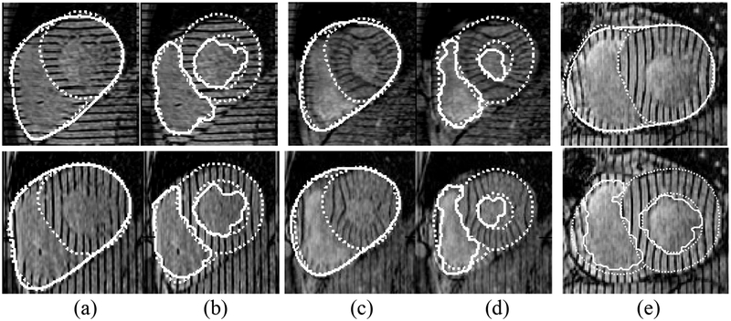
For qualitative validation we compare the segmented bi-ventricular boundaries to those drawn by expert cardiologists (see Fig. 8a–d). These boundaries are shown for several slices at time 2 and time ES. By superimposing both boundaries over the images and enlarging them we find convincing evidence of the accuracy of our algorithm. We have also discovered cases (see Fig. 8e) in which the cardiologists have found our algorithm to be more accurate than those drawn by hand, causing us to have the anatomists revise the ground truth contours.

Fig. 8.

Qualitative validation: segmented contours (solid lines), manual contours (dotted lines). Epicardium (a) and endocardium (b) contours from two slices at time 2. Epicardium (c) and endocardium (d) contours from the same two slices at time ES. Note that our algorithm finds one epicardium contour while two manual contours (LV and RV epicardium contours have been drawn). Also our algorithm includes papillary muscle in the myocardium while the manual contour excludes it. Shown in (e) top row is a case in which our algorithm was more accurate than manual contours along the RV. Bottom row: endocardium contours segmenting the papillary muscle

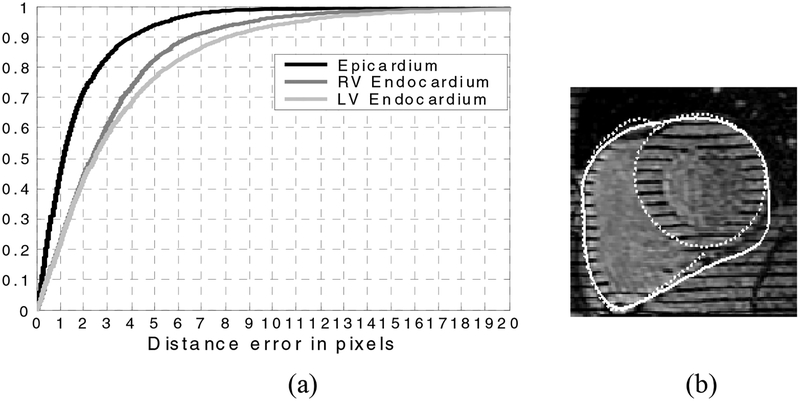
For quantitative validation we compute the distance between each segmented contour A and the corresponding contour, B, drawn by the expert anatomist by computing the distance $d(a,B)=\underset{b\in B}{\text{min}}\Vert a-b\Vert$ for all points a on the automatic contour. We also compute d(b, A) for the points, b on the expert contours. Fig. 9 shows the cumulative distribution of these error distances for the contour points over all slices in all volumes from ED (end diastole) to ES (end systole) for the normal and diseased subjects comprising over 175 images. To validate the segmented RV endocardium we use the full manually drawn RV endocardium and the portion of the LV epicardium that delineates the septum. Likewise during validation of the segmented single epicardium contour we use the full manual RV epicardium contour and the portion of the LV epicardium corresponding to the non-septum boundary. It can be seen (Fig. 9) that on the average the distance error of our segmented epicardium contour is less than 1.2 pixels and that 90% of the time the error is less than 4.1 pixels. The endocardium contours are still quite accurate although our contours include the papillary muscle in the myocardium while the manually drawn contours have excluded them, thus the “error” distance is larger. For the RV endocardium we still find though that on the average the distances are less than 2.3 pixels and 90% of the time the segmented contour is within 6.5 pixels of the expert’s contour.

Fig. 9.

(a) Cumulative distribution of distances errors between the corresponding portions of the expert manual contours and the segmented contours from all slices, in all volumes, from ED through ES. (b) Occasionally the epicardium boundary is too weak after the tags are filled via the morphological closing. Then the active contour can expand beyond the myocardium, so we are developing ways to correct this case (see text)

There is still room for improvement. Our quantitative results include time 1 (end-diastole). For this volume the tags have not washed away completely so we have used the endocardium contours from time 2 and used them to initialize our active contour that locates the epicardium at time 1. Using an active contour for both the endocardium segmentation (using the grayscale opened images) and the epicardium segmentation will enable us to estimate the velocity of the endocardium contour relative to the epicardium contour. Inverting the motion will give us an improved endocardium estimate for time 1. We are also experimenting with improved edge sensitivity that can handle the occasional leakage (see Fig 9b) of the epicardium contour into the liver.

6. Conclusions

We have presented a method that dramatically reduces the most significant portion of the analysis time required to process SPAMM data. All of the steps in our algorithm are completely automated, requiring no user input. The contours can be used to measure ejection fraction and as a basis to register motion fields derived from tag tracking algorithms which enables effective inter-subject comparison of motion data. The algorithm removes background intensity variation throughout each imaged volume using a new scale based intensity correction method and implements a novel region-based segmentation technique to segment the ventricular blood filled volumes and the LV and RV endocardium contours. We have also located the inflow and outflow tracts of the right ventricle automatically and obtained excellent epicardium results through a combination of adaptive local statistics-based image filtering, a gradient vector flow field and physics-based active contours.

References

- 1.Axel L, Dougherty L, “Heart wall motion: improved method of spatial modulation of magnetization for MR imaging”, Radiology, 172, 349–350 [DOI] [PubMed] [Google Scholar]
- 2.Zerhouni E, Parish D, Rogers W, et al. , “Human heart: tagging with MR imaging-a method for non-invasive assessment of myocardial motion”, Radiology, 169, 59–63 [DOI] [PubMed] [Google Scholar]
- 3.Kraitchman D, Young A, Chang C, Axel L, “Semi-automated tracking of myocardial motion in MR tagged images”, IEEE Transactions on Medical Imaging, 14, 422–433, 1995 [DOI] [PubMed] [Google Scholar]
- 4.Young, “Model Tags: Direct 3D tracking of heart wall motion from tagged magnetic resonance images.” Medical Image Analysis. 3:361–372, 1999 [DOI] [PubMed] [Google Scholar]
- 5.Denney T Jr., “Estimation and Detection of Myocardial Tags in MR images without User Defined Myocardial Contours”, IEEE Transactions on Medical Imaging, 1999 [DOI] [PubMed] [Google Scholar]
- 6.Osman N, Kerwin W, McVeigh E, and Prince J, “Cardiac Motion Tracking Using CINE Harmonic Phase (HARP) Magnetic Resonance Imaging” Technical Report JHU/ECE 99–3, Electrical and Computer Eng, Johns Hopkins Univ. [DOI] [PMC free article] [PubMed] [Google Scholar]
- 7.Kerwin W, Osman N, Prince J, “Ch 24: Image Processing and Analysis in Tagged Cardiac MRI”, Handbook of Medical Imaging: Processing and Analysis, Editor-in-chief Bankman I, 2000 [Google Scholar]
- 8.Chen Y, Amini A, “A MAP Framework for Tag Line Detection in SPAMM Data Using Markov Random Fields on the B-Spline Solid”, IEEE Workshop on Mathematical Methods in Biomedical Image Analysis, December 2001 [DOI] [PubMed] [Google Scholar]
- 9.Haber, “Three-dimensional motion reconstruction and analysis of the right ventricle from planar tagged MRI”, Univ. of Penn. PhD Thesis, 2000 [DOI] [PubMed] [Google Scholar]
- 10.Park J, Metaxas D, Young A, Axel L, “Deformable models with Parameter Functions for Cardiac Motion Analysis” IEEE Transactions on Medical Imaging, Vol. 15, No 3, June 1996 [DOI] [PubMed] [Google Scholar]
- 11.Declerck J, Ayache N, McVeigh E, “Use of a 4d Planispheric Transformation for the Tracking and Analysis of LV Motion with Tagged MR Images”, 1999 [Google Scholar]
- 12.Ozturk C, McVeigh E, “Four Dimensional B-spline Based Motion Analysis of Tagged Cardiac MR Images”, Proc. SPIE Medical Imaging 99, San Diego, CA, February 1999. [Google Scholar]
- 13.Guttman M, Prince J, McVeigh E, “Tag and Contour Detection in Tagged MR Images of the Left Ventricle”, IEEE transactions on Medical Imaging, 13(1): 74–88, 1994 [DOI] [PubMed] [Google Scholar]
- 14.Goutsias J, Batman S, “Ch 4: Morphological Methods for Biomedical Image Analysis”, Editors Sonka M, Fitzpatrick J, Handbook of Medical Imaging, Vol. 2. Medical Imaging Processing and Analysis, pp 255–263, SPIE, 2000 [Google Scholar]
- 15.Zhuge Y, Udupa J, Liu J, Saha P, Iwanaga T, “A Scale-Based Method for Correcting Background Intensity Variation in Acquired Images”, SPIE Proceedings, 2002 [Google Scholar]
- 16.Dann R, Hoford J, Kovacic S, Reivich M, Bajcsy R, “Evaluation of Elastic Matching System for Anatomic (CT, MR) and Functional (PET) Cerebral Images”, J. of Computer Assisted Tomography, 13(4) 603–611 July/August, 1989 [DOI] [PubMed] [Google Scholar]
- 17.Kass M, Witkin A, Terzopoulos D, “Snakes: Active contour models”, International Journal of Computer Vision, 2:321–331, 1988 [Google Scholar]
- 18.Xu J. Prince, “Generalized Gradient Vector Flow External Forces for Active Contours”, Signal Processing 71, pp 131–139, 1998 [Google Scholar]