Spatial Regression Analysis of Poverty in R

Abstract

Poverty has been studied across many social science disciplines, resulting in a large body of literature. Scholars of poverty research have long recognized that the poor are not uniformly distributed across space. Understanding the spatial aspect of poverty is important because it helps us understand place-based structural inequalities. There are many spatial regression models, but there is a learning curve to learn and apply them to poverty research. This manuscript aims to introduce the concepts of spatial regression modeling and walk the reader through the steps of conducting poverty research using R: standard exploratory data analysis, standard linear regression, neighborhood structure and spatial weight matrix, exploratory spatial data analysis, and spatial linear regression. We also discuss the spatial heterogeneity and spatial panel aspects of poverty. We provide code for data analysis in the R environment and readers can modify it for their own data analyses. We also present results in their raw format to help readers become familiar with the R environment.

1. Introduction

Throughout human history, poverty has been associated with many social problems and historic events, including inequality, wars, and revolutions. Even in developed countries, poverty persists. Thus, it is not a surprise that poverty is a topic that has been studied across many social science disciplines, generating a large body of literature. Poverty, like many other social phenomena, can be spatial and scholars of poverty research have long recognized that the poor are not uniformly distributed across space (Nord, Luloff, and Jensen 1995; Thiede, Kim, and Valasik 2018; Voss et al. 2006; Weber et al. 2005). Understanding the spatial distribution of poverty helps us to understand place-based structural inequalities (Lobao, Hooks, and Tickamyer 2008; Tickamyer and Duncan 1990). This school of research is also referred to as the study of “place poverty,” in contrast with “people poverty,” as the former emphasizes structural and contextual forces while the latter emphasizes individual or family forces (Voss et al. 2006).

The spatial aspect of poverty has been increasingly studied using formal spatial analysis and spatial regression models (e.g., Curtis et al. 2018; Curtis, Voss, and Long 2012). While the methods are many, there is a learning curve to learn and apply them to poverty research. This manuscript aims to introduce the concepts of spatial regression modeling and walk the reader through the steps of conducting poverty research using R, an open-source statistical software that is gaining increasing popularity among social scientists (R Development Core Team 2008). Similar to other teaching notes (Sparks 2013a, 2013b), we provide code for data analysis in the R environment and readers can modify it for their own data analyses. We also present results in their raw format to help readers become familiar with the R environment. Poverty research has been reviewed in several articles and books (e.g., Iceland 2013; Duncan 1992; Jennings 1999; Sandoval et al. 2009; Weber et al. 2005) and thus is not reviewed in this manuscript. Readers are suggested to refer to these review articles for the status of poverty research.

In the following sections, we introduce our data (Section 2), walk the readers through the steps of exploratory data analysis (Section 3), standard linear regression (Section 4), neighborhood structure and spatial weight matrix (Section 5), exploratory spatial data analysis (Section 6), and spatial linear regression (Section 7), all in R, and discuss other spatial aspects of poverty that could be addressed (Section 8).

2. Data and Units of Analysis

This manuscript provides an example in R of quantifying the spatial relationship between county-level poverty rates and several socioeconomic factors in the 48 states of the contiguous United States. Among the existing place poverty studies, county is often used as the unit of analysis; counties are salient units in policy making and planning perspectives such that many policy decisions potentially relevant to poverty rates are made at the county level (Greenlee and Howe 2009; Lichter and Johnson 2007; Thiede et al. 2018; Voss et al. 2006). Moreover, compared with the boundaries of other administrative units, county boundaries are subject to little boundary change, therefore facilitating scholarly study of poverty trends over time. Studies have found that county-level poverty is associated with many other structural disadvantages, especially when it comes to some major health indicators, such as cancer stage (Greenlee and Howe 2009), obesity (Bennett, Probst, and Pumkam 2011), and HIV prevalence (Vaughan et al. 2014). Commonly identified factors associated with the spatial concentration of county-level poverty rates include economic structure (Goetz and Swaminathan 2006; Lobao et al. 2008), racial composition (Thiede et al. 2018; Wimberley and Morris 2002), and human capital stock (Levernier, Partridge, and Rickman 2000).

The variable of interest is poverty (povty), measured as the percentage of individuals age 18–64 living in poverty in a county in year 2000. We include a set of economic, social, and demographic factors that may relate with county-level poverty rates. Specifically, three variables, agriculture (ag), manufacturing (manu), and retail (retail), are the percentages of workers in the agricultural sector, the manufacturing sector, and the retail sector, respectively. For socially-related factors, foreign is the percentage of the foreign-born population in a county and female employment (feemp) is the percentage of female employment in the total population. Human capital stock is captured by high school (hsch), which indicates the percentage of the population that completed a high school education. Lastly, we use percentage Blacks (black) and percentage Hispanics (hisp) to capture racial and ethnic compositions. These variables are measured in 2000 based on the Decennial Census data. We download the data using SocialExplorer, an online demographic research tool that pre-processed the raw Census data and reports calculated percentages by county. While other variables have been used in poverty research, in this manuscript we focus on these selected variables for the purpose of illustrating spatial regression modeling for poverty research in R. We have made the dataset (uspoverty2000.csv) and supplementary tutorials available at https://mkamenet3.github.io/SpatialRegPovertyR/.

3. Standard Exploratory Data Analysis

After initial installation, we first load the R libraries that the analysis needs.

After the census data are downloaded and the variables of interest are extracted, we streamline the data and save them to a proper data file to be read into R as a data frame before performing statistical data analysis. We use the read_csv() function from the readr package to import the csv file into R and to specify that the variable FIPS_N is imported as a character variable (col_types = cols(FIPS_N = col_character())) and that the import does not omit leading zeros from FIPS_N variable (trim_ws = FALSE). We immediately pipe (%>%) to the arrange() function from the dplyr package to sort by FIPS_N.

The counties are identified by their five-digit federal information processing (FIP) standards code, with the first two digits corresponding to a state code and the last three digits corresponding to a county code. The data frame povdf features the poverty rate and the socioeconomic variables from the census year 2000 in the 3,070 counties of the 48 contiguous states. Using the R function head(), we view the first six counties in the data frame povdf:

To perform exploratory data analysis, we use summary statistics and graphical methods. Most commonly used summary statistics and graphical methods for exploratory data analysis are applied to either one variable at a time (i.e., univariate) or two variables at a time (i.e., bivariate). Using the R function summary(), we obtain several univariate summary statistics for each of the variables in the data frame povdf:

For a continuous variable, the summary statistics are its minimum, first quartile, median, mean, third quartile, and maximum. The summary statistics of the response variable of poverty rate show that the lowest county-level poverty rate was 2.04% and the highest county-level poverty rate was 53.83% among the 3,070 counties in the contiguous United States in 2000. The center of the county-level poverty rates is 11.61% measured by median and 12.69% measured by mean (i.e., average). In addition, the interquartile range is between the first quartile of 8.51% and the third quartile of 15.70%. That is, half of the counties had poverty rates below 11.61% and the other half had poverty rates above 11.61%, while the middle half of the counties had poverty rates between 8.51% and 15.70%. Among the explanatory variables, we use female employment rate as an example. The summary statistics of the female employment rate tell us that county-level female employment rates ranged between the lowest at 23.21% and the highest at 78.47% among the 3,070 counties in the contiguous United States in 2000. Half of the counties had female employment rates below the median of 51.88% and the other half had female employment rates above 51.88%, while the middle half of the counties had female employment rates between 46.94% and 56.30%.

Using the R function cor(), we obtain the sample correlation, a bivariate summary statistic, between poverty rate and any given socioeconomic factor. For example, the correlation between poverty rate and female employment rate is:

The sign of this sample correlation is negative, indicating a negative correlation between the poverty and female employment rates. That is, higher female employment rates are associated with lower poverty rates, whereas lower female employment rates are associated with higher poverty rates. The magnitude of this correlation is 0.69 (rounded from 0.6900635) and reflects a moderate amount of association between the poverty and female employment rates for such an observational study in the social sciences.

Among the many graphical methods used for exploratory data analysis, in this manuscript we demonstrate two often-used graphs, one univariate and the other bivariate. In particular, we draw a histogram and a scatter plot by the ggplot2 R package, using the geometries, geom_histogram() and geom_point(), respectively:

Figure 1 shows the histogram of povty and the scatter plot for povty by feemp. The histogram shows that the range of poverty rates is between 0 and 55% with a center around 10% (Figure 1a). The histogram is also right skewed, revealing counties with high poverty rates in the right tail. The histogram is based on density such that the areas of the vertical bars at 5% increments add up to a total probability of 1. Alternatively, we could plot the histogram by the number of counties at the 5% increments and the shape of the histogram would be the same.

Figure 1.

Histogram of poverty (a) and scatter plot between the poverty rate and the female employment rate (b)

The scatter plot shows a negative trend (Figure 1b). As the female employment rate increases from 20% to nearly 80%, the poverty rate declines. This finding is consistent with the negative sample correlation, indicating a negative association between female employment rate and poverty rate.

4. Standard Linear Regression

4.1. Model Fitting

To quantify the relationships between the poverty rate and the socioeconomic variables, we perform standard linear regression such that the response variable is poverty rate and the eight explanatory variables are percentage of agricultural workers (ag), percentage of manufacturing workers (manu), percentage of retail workers (retail), percentage of foreign-born residents (foreign), percentage of female employment (feemp), percentage of high school graduates (hsch), percentage of Blacks (black), and percentage of Hispanics (hisp).

The analysis in the remainder of this note focuses on interpretation and relies on the large sample size of exploring all counties in the continental United States (3,070 counties). Given that our response ranges from 0–100% and that the models in this analysis are linear models, it is possible that fitted values may lie outside of the range leading to predictions of negative poverty or poverty over 100%. In the interest of interpretability and because consideration of appropriate transformations depends on a case by case basis, we do not use any transformations to address this. For smaller area studies, we encourage the reader to consider linear transformation of the response (ex: logit, log, square root, arcsine) in order to meet the normality assumptions imposed by these models. Weighting by the population size may also be explored. Supplementary tutorials can be found at https://mkamenet3.github.io/SpatialRegPovertyR/.

The R function lm() is applied to the data frame povty and the output m1 is an lm object. We then apply the R function summary() to the m1 object and obtain the results of the standard linear regression:

There are four parts to the summary of this standard linear regression. The initial function call is echoed in the first part. The second part reports the summary statistics of residuals (minimum, first quartile, median, third quartile, and maximum). Here the residual is defined as the difference between an observed response (poverty rate) and its fitted value by the linear regression. We use residuals for model diagnostics near the end of this subsection. The third part reports, for each explanatory variable, a fitted regression coefficient (under Estimate), its standard errors (under Std. Error), the ratio of the two values as a T test statistic (under t value), and a p-value for testing whether the true regression coefficient is zero or not (under Pr(>|t|)). For example, the estimated regression coefficient for feemp is −0.526 (rounded from −0.52635676) with standard error 0.011166. The T test statistic is −47.141 and the p-value is <2E–16. This tells us that a 1% increase in the female employment rate is associated with a 0.526% decrease in the poverty rate when all other explanatory variables are held constant. How significant is this result? Relative to the standard error of about 1.12%, the T statistic is very large and the p-value is extremely small. There is very strong evidence that the true regression coefficient for female employment rate is not zero. The last part of the output provides a residual standard 3.809 on 3061 degrees of freedom, which estimates the standard deviation of the error term in the standard linear regression model. In addition, a multiple and an adjusted R-squared are reported, indicating that about 58% of the variation in the response variable of poverty rate is explained by the relationship with the socioeconomic variables considered herein. Finally, an F-test is carried out for testing whether all of the regression coefficients are zero. The p-value is <2.2E–16 and there is very strong evidence that the not all the regression coefficients are zero.

In addition, we may extract the estimated regression coefficients and the corresponding 95% confidence intervals by applying the R functions coef() and confint() to the m1 object. By the R function cbind() below, we combine these results into a table of three columns, one for the estimated regression coefficients (named coefest) and the other two for the lower and upper limits of the 95% confidence intervals.

For example, the estimated regression coefficient for feemp is −0.526 with a 95% confidence interval of [−0.548, −0.504]. That is, there is a 95% confidence of between 0.504% and 0.548% decrease in the poverty rate associated with a 1% increase in the female employment rate when all other explanatory variables are held constant.

4.2. Model Selection

Among the socioeconomic explanatory variables, one of them, retail, is not significant (p-value = 0.10458). It is common practice to perform model selection in search of a more parsimonious model that has possibly fewer explanatory variables. We use the R function step() to perform a backward elimination based on Akaike’s information criterion (AIC) and save the result to an lm object m2. That is, we start with the full model m1, which has all the socioeconomic explanatory variables, and we drop the explanatory variable that results in the largest decrease in AIC iteratively until there is no further decrease in AIC. Recall that a smaller AIC indicates a better model fit balanced with model parsimony. It should be noted that the stepwise exercise could result in biased p-values and thus should be avoided when possible.

When the explanatory variable retail is dropped, the AIC value increases from 8219.8 to 8220.5. This indicates that the model without retail is not as good a model as the full model with all the explanatory variables m1. This holds for all the other explanatory variables as well, and thus none of the explanatory variables are dropped from the full model based on AIC. The final model m2 is the same as the full model m1.

Alternatively, we could use the R function step() to perform backward elimination based on Schwartz’s Bayesian information criterion (BIC) by setting the penalty coefficient to the log of the sample size (k=log(n)) and save the result to an lm object m3. Like AIC, a smaller BIC indicates a good model fit balanced with model parsimony. We thus start with the full model m1, which has all the socioeconomic explanatory variables, and we drop the explanatory variable that results in the largest decrease in BIC iteratively until there is no further decrease in BIC:

There are three steps in this model selection by BIC. In the first step, the retail explanatory variable is dropped from the reference model with all the explanatory variables because the BIC value of 8268.7 without retail is smaller than the BIC value of 8274.1 for the reference model with retail, whereas dropping any of the other explanatory variables would result in a BIC value larger than 8274.1 for the reference model. In the second step, the reference model without retail has a BIC value of 8268.7 and the manu explanatory variable is dropped because the BIC value of 8267.7 without manu is smaller than the BIC value of 8268.7 for the reference model with manu, whereas dropping any of the other explanatory variables would result in a BIC value larger than 8268.7 for the reference model. In the third and last step, the reference model without retail and manu has a BIC value of 8267.7. Because leaving out any of the remaining explanatory variables would result in an increase in the BIC value, the model selection is finished. The final best model is m3 without retail and manu, with the following summary of the model fit:

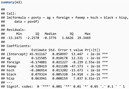
This standard linear regression summary for m3 provides estimates for the regression coefficients that are similar to those of m1. For example, in m3 the estimated regression coefficient for feemp is −0.528 with standard error 0.011108, compared with an estimate of −0.526 with standard error 0.011166 in m1. There is a very slight decrease of the multiple and the adjusted R-squared values, but the amount of variation in the response variable explained by this final best model remains about 58%. We proceed with this set of six explanatory variables (ag, foreign, feemp, hsch, black, and hisp) in the remainder of this manuscript.

4.3. Model Diagnostics

Now that we have fitted standard linear regression models and selected a final model m3, we perform model diagnostics for the purpose of evaluating the model assumptions. There are four model assumptions to evaluate: linearity, independence, equal variance, and normality. For linearity and equal variance, it is common to use the plot of residuals versus fitted responses. This is the first option in the R function plot() applied to m3 (plot(m3, which=1)). For normality, it is common to use the normal quantile-quantile (QQ) plot of the standardized residuals, which is the second option in the R function plot() applied to m3 (plot(m3, which=2)). These two plots can also be created using ggplot2. For the residuals versus fitted response, we extract the fitted and residual values from m3 and use geom_smooth() layered over geom_point() to create the plot. For the QQ plot, we extract the standardized residuals from m3 and use stat_qq_line() layered over geom_qq() to create the plot.

The normal Q-Q plot (Figure 2a) shows a departure from the straight line at the upper end, indicating right skewness in the residuals (i.e., more large positive residuals than a normal distribution would typically have). The right skewness is also reflected in the plot of the residuals versus the fitted responses (Figure 2b), while the remaining residuals appear to be scattered fairly randomly.

Figure 2.

Quantile-quantile (Q-Q) plot of the standard linear regression model residuals

When model diagnostics like those above indicate any departure from the standard linear regression assumptions, remedial measures are not always needed due to the robustness of the regression. When remedial measures are needed, a commonly used approach is transformation of the response variable and/or the explanatory variables. For illustration, we take the logit transformation of the response variable ($log\left(\frac{p}{1-p}\right)$) and fit a linear regression model. We use the logit() function from the car package as it adjusts proportions that are perfectly 0 or 1. Then we perform model diagnostics as before by a residual versus fitted response plot and a normal QQ plot (Figure 3):

Figure 3.

Quantile-quantile (Q-Q) plot of the standard linear regression model residuals with the response variable transformed

The normal Q-Q plot (Figure 3a) shows less departure from the straight line at the upper end but more departure at the lower end, indicating a possible overcorrection of the right skewness in the untransformed data. In the plot of the residuals versus the fitted responses (Figure 3b), several large negative residuals are marked and there is some indication of smaller variance for larger fitted values (i.e., unequal variance). This example demonstrates some of the challenges in model selection and model diagnostics. Taking a remedial measure to correct the departure from one assumption could lead to the departure from another assumption. For the remainder of this manuscript, we model the original poverty rate without any transformation.

Thus far we have evaluated the assumptions of linearity, equal variance, and normality. The independence assumption, however, is not an option in the R function plot(); we evaluate the independence assumption in Section 7.1.

5. Neighborhood Structure and Spatial Weight Matrix

In Sections 3 and 4, we performed exploratory data analysis and standard linear regression analysis of the poverty rate data without considering spatial information in the data. In this section, we create a neighborhood structure and a spatial weight matrix in preparation for spatial analysis. In the following two sections, we perform exploratory spatial data analysis (Section 6) and carry out spatial regression analysis (Section 7).

Recall that the data frame povdf comprises of the response variable and the explanatory variables as well as the FIP code that identifies the counties in the 48 states of the contiguous United States.

We now create neighbors and their corresponding spatial weights. First, we import U.S. counties shape file into R using the counties() function from the tigris package. In order to only import counties that correspond to the counties in the poverty data set povdf (the contiguous United States), we specify (state = povdf$STATEFP). We set the resolution of the shape file to be 500k with (cb=TRUE) and the census year for the shape files to be 2000. The county shape files are automatically imported into a SpatialPolygonsDataFrame. For faster performance and easier manipulation, we convert uscounties to a “simple features” data frame using the st_as_sf() function from the sf() package.

Now that we have the counties prepared, we need to connect the counties to the povdf data frame. To merge the two data frames, we use the merge() function. Prior to merging, we first create the data vector FIPS_N by combining the state and county FIPs codes and set it as a variable in the uscounties_sf data frame. This gives us a unique identifier for each county which we can merge with FIPS_N from the povdf data frame.

The object povdf_uscounties_sf is both a simple features (sf) object and a data.frame, being associated multi-polygon geometries. In order to create the neighborhood structure of counties in the continental United States, we use the poly2nb() function from the spdep package. We first coerce povdf_uscounties_sf to a SpatialPolygonsDataFrame using the as_Spatial() function (from the sf package) and specify IDs = povdf_uscounties_sf$FIPS_N. After setting the row names of povdf_uscounties_spdf to be the row names of the povdf data frame, we apply poly2nb().

The output pov_nb is a neighborhood object which explicitly lists who are neighbors with whom and, in our case, which county is a neighbor with which county. We then create spatial weights by the R function nb2listw() from the spdep package (Bivand et al. 2013) using the default option of row standardization (style=“W”) and binary weights (style=“B”):

We specify zero.policy=TRUE above because some counties do not have any neighbors, such as Nantucket County in Massachusetts, and the neighborhood object pov_nb has entries that are null. The zero policy allows spatial weights to be created for counties with one or more neighbors despite the null entries. The output listw_povB is a spatial weight object, which can be visualized by a map as shown in Figure 4. The plot() function applied to a list of spatial weights takes the list of spatial weights and coordinates of the centroids as arguments. We extract geometries of the county polygons using st_geometry(), the centroids using st_centroid(), and finally the coordinates using st_coordinates().

Figure 4.

Neighborhood structure

The centroids of all pairs of neighboring counties are connected by a line and the map can be thought of as a network or a graph such that the county centroids are the vertexes and the connecting lines between neighboring counties are the edges.

6. Exploratory Spatial Data Analysis

We performed exploratory data analysis by summary statistics and graphical methods in Section 4. However, standard exploratory data analysis does not take into account the spatial nature of the data. In this section we consider exploratory spatial data analysis by summary statistics and graphical methods that utilize the spatial information in the data. The goal of exploratory spatial data analysis is for the reader to gain insights into the spatial nature of their data as a way to inform them how best to proceed with their choice of model, determination of outliers, and scope of the inferences that can be made from the data via confirmatory analysis. A natural graphical method to use for exploratory spatial data analysis is a heat map, where the levels of a variable are color coded on a map. We can draw the heat map of the poverty rates as well as heat maps of the socioeconomic explanatory variables over the 3,070 counties in the contiguous United States.

We use ggplot2 to plot the response variable, povty, by passing the sf data frame povdf_uscounties_sf to the ggplot() function. We add the geometry geom_sf() and specify the aesthetic aes(fill=povty). Additional features specify the black and white plot theme (theme_bw()) and the grey color scale ((scale_fill_continuous(low=“white”, high=“black”))).

For illustration, we use ggplot() to plot one of the explanatory variables, female employment rate feemp.

The spatial pattern of povty (Figure 5a) indicates relatively low poverty rates in the northern and western states, whereas the poverty rates are relatively high in the southeastern states. The spatial pattern of feemp (Figure 5b) indicates relatively high female employment rates in eastern states. The relationship between poverty and female employment rates shown in Figure 5 is not as obvious as in Figure 1.

Figure 5.

Poverty rate (a) and female employment rate (b) in 2000

It should be noted that the tmap R package and extensions can also be used to create high quality thematic maps. We provide a supplementary tutorial online (https://mkamenet3.github.io/SpatialRegPovertyR/) and encourage the reader to further explore spatial visualizations using tmap (Lovelace et al. 2019).

6.1. Moran’s I and Geary’s c

For exploratory spatial data analysis, summary statistics such as Moran’s I and Geary’s c can be used to quantify spatial dependence. With the neighborhoods created in Section 5, we use the R function moran.test() to estimate the Moran’s I statistic and perform a Moran’s I test for the null hypothesis that there is no spatial dependence versus a two-sided alternative hypothesis that there is spatial dependence:

Based on the output above, the Moran’s I statistic is 0.5669, indicating positive spatial dependence among neighboring counties. If there is no spatial dependence, then the expected value and the variance of the Moran’s I statistic are –0.000326 and 0.0001106, respectively. This results in a standard deviation (or Z-value) of 53.934 with a p-value less than 2.2E–16 (i.e., 2.2×10⁻¹⁶), which is virtually zero. There is very strong evidence for spatial dependence in the poverty rates across counties in the continental U.S.

The Moran’s I test by moran.test() is based on a normal approximation and the variance estimation is based on randomization. Alternatively, a Monte Carlo test can be performed by the R function moran.mc(), where we pre-specify the number of Monte Carlo simulations (here, nsim=999) and compare the Moran’s I statistic of 0.5669 against the null distribution of the Moran’s I statistic under the assumption of no spatial dependence. We set the randomization seed to 1 so that when the code is re-run we get the same test result:

This Monto Carlo test shows that the rank of the observed Moran’s I test statistic of 0.5664 is larger than any of the test statistics from the nsim=999 simulations and thus has the highest rank. The p-value is 1 out of 1000, which is 0.001 for a null hypothesis that there is no spatial dependence versus a one-sided alternative that there is positive spatial dependence. That is, there is very strong evidence for positive spatial dependence in the poverty rates among counties. For a two-sided alternative that there is spatial dependence (positive or negative), we double 0.001 and obtain a p-value of 0.002. There is still very strong evidence for spatial dependence in the poverty rates among counties.

Besides Moran’s I, we may use the R function geary.test() to estimate the Geary’s c statistic and perform a Geary’s c test for the null hypothesis that there is no spatial dependence versus a two-sided alternative hypothesis that there is spatial dependence:

Based on this output, the Geary’s c statistic is 0.4288, indicating a positive spatial dependence among neighboring counties. If there were no spatial dependence, the expected value and the variance of the Geary’s c statistic would be 1 and 0.0001968, respectively. This results in a standard deviation (or Z-value) of 40.714 with a p-value that is also virtually zero. There is again very strong evidence for spatial dependence in the poverty rates across counties.

The Geary’s c test by geary.test() is based on a normal approximation and the variance estimation is based on randomization. Alternatively, a Monte Carlo test can be performed by the R function geary.mc(), where we pre-specify the number of Monte Carlo simulations (by nsim=999) and compare the Geary’s c statistic of 0.4288 against its null distribution under the assumption of no spatial dependence:

This Monto Carlo test shows that the rank of the observed Geary’s c test statistic of 0.42879 is larger than any of the test statistics from the nsim=999 simulations and thus ranks the highest. The p-value is thus 0.002 (0.001) for a two-sided (one-sided) alternative and there is very strong evidence for spatial dependence (positive spatial dependence) in the poverty rates across counties.

6.2. Local Moran’s I

To apply local Moran’s I to the data, we use the R function localmoran() from the spdep package. The output is extensive, so here we apply the R function head() to take a look at the first six counties as an example. We also use the R function round() to round the output values to two digits after the decimal point:

For example, for the county identified by FIPS_N 01001 in the output above (Autauga County, Alabama), the local Moran’s I (Ii) is −4.99, with virtually zero expectation (E.Ii) and a variance of 4.99 (Var.Ii). Thus, the standard deviate (Z.Ii) is –1.24 and the p-value (1-Pr(z>0)) is 1–0.89=0.11 for a one-sided alternative (the p-value is 0.22 for a two-sided alternative). There is no evidence of local spatial dependence for this county.

7. Spatial Linear Regression

7.1. Diagnostics for Spatial Dependence

In Section 4, we fitted and selected standard linear regression models to quantify the relationship between poverty rates and socioeconomic variables. We also carried out model diagnostics using residuals plots to evaluate the model assumptions of linearity, equal variance, and normality (but not yet independence). We are now ready to evaluate the independence assumption.

Here we use row-standardized spatial weights and recall the spatial weights object listw_povW. We apply the R function lm.morantest() to the residuals of the fitted standard linear regression models. The null hypothesis is that there is no spatial dependence in the error term of the standard linear regression model.

Based on the output above, the Moran’s I statistic is 0.2701, indicating a positive spatial dependence among neighboring counties. The standard deviation (or Z-value) is 25.358 with a p-value less than 2.2E–16, which is virtually zero. There is very strong evidence for spatial dependence among the errors of the standard linear regression model. This calls for more complex spatial linear regression analysis. The next subsection presents spatial lag models and spatial error models including the simultaneous autoregressive (SAR) and conditional autoregressive (CAR) models.

7.2. Spatial Lag Models

We consider fitting a spatial lag model to the poverty rates data. The R function lagsarlm() is applied to the data frame povdf and the output is m3_lag.

Coefficients estimated from spatial lag models cannot be interpreted directly because of spillovers between the terms in the data generation process. We refer the reader to Golgher et al. (2016) regarding spatial confounding and spillover effects. We calculate impacts using the impacts() function from the spdep package.

The output gives us the direct (or local) effect, indirect (or spillover) effect, and total effect (or sum of the direct and indirect effects). The total effect can be interpreted similarly to our interpretation of regression coefficients in the standard linear model. The total effect of feemp is −0.616 (rounded from −0.61628131). A 1% increase in female employment is associated with a 0.616% decrease in poverty.

There are five parts to this spatial linear regression output. The initial function call is in the first part. The second part reports the summary statistics of residuals (minimum, first quartile, median, third quartile, and maximum). Here the residual is defined as the difference between an observed response and its fitted value by the spatial linear regression. The third part reports, for each explanatory variable, a fitted regression coefficient (under Estimate), its standard errors (under Std. Error), the ratio of the two values as a Z test statistic (under z value), and a p-value for testing whether the true regression coefficient is zero or not (under Pr(>|z|)). For the spatial lag model, we use the impacts to assess coefficient estimates. For example, the estimated regression coefficient for feemp is −0.378 with standard error 0.01262. The Z test statistic is −29.9495 and the p-value is less than 2.2E–16. This tells us that a 1% increase in the female employment rate is associated with a 0.378% decrease in the poverty rate when all other explanatory variables are held constant. Relative to the standard error of about 1.262%, the Z statistic −29.9495 is very large and the p-value is extremely small. There is very strong evidence that the true regression coefficient for female employment rate is not zero.

The fourth part of the output provides the estimate of the spatial correlation coefficient rho, which is 0.387. Two hypothesis tests—a likelihood ratio (LR) test and a Wald test—are applied for testing whether the true spatial correlation coefficient rho is zero or not. The LR test value is 409.57 with a p-value of less than 2.2E–16 . The Wald test is presented as a Z test with a z-value of 20.502 and a p-value of less than 2.2E–16. Equivalently, the Wald test statistic is 420.35, which is the square of the z-value, and the p-value of less than 2.2E–16 is the same as the Z test. Both the LR test and the Wald test indicate there is very strong evidence that the spatial correlation coefficient rho is not zero.

The fifth and last part of the output provides several useful statistics and tests. The log-likelihood value for the fitted spatial lag model is −8257.118 and the AIC value is 16532, which is smaller than the AIC value of 16940 for the standard linear regression model. The maximum likelihood estimate of the error variance sigma squared is 12.334, with the error standard deviation sigma estimated to be its square root, 3.512. Finally, the Lagrange multiplier (LM) test for the spatial dependence in the error term has a test value of 47.6 and a small p-value, indicating that there is additional spatial dependence unaccounted for by the spatial lag model.

We have already tested for spatial dependence in the error term and learned that there is strong evidence for spatial dependence. In addition, we may plot the residuals against the fitted responses (Figure 6) as follows:

Figure 6.

Fitted values versus residuals of the spatial lag model

From the residual plot (Figure 6), we see that the residuals are distributed fairly randomly around the zero horizontal line and the variation tends to be higher for larger fitted values. This suggests no obvious departure from the linearity assumption, but there is indication of unequal variances among the errors.

We apply the Breusch-Pagan (BP) test for the null hypothesis that the error variance is constant versus the alternative that the error variance is not constant by the R function bptest.sarlm():

The observed BP test statistic is 218.63 and the p-value is extremely small. There is very strong evidence for unequal variance in the error term of the spatial lag model.

7.3. Spatial Durbin Error Models

As an alternative to the spatial lag model, we consider fitting a spatial Durbin error model to the poverty rates data. The R function errorsarlm() is applied to the data frame povdf and the option Durbin is to TRUE to specify the Durbin error model. The output is m3_err. We then apply the R function summary() to the m3_err object and obtain the results of the spatial error model fit:

There are five parts to this spatial linear regression output. The initial function call is in the first part. The second part reports the summary statistics of residuals (minimum, first quartile, median, third quartile, and maximum. The third part reports each explanatory and fitted coefficients. However, these cannot be directly interpreted due to the spatial lag in the model. As with the spatial lag model, we use the impacts to assess coefficient estimates in this spatial Durbin error model because there is a spatial lag in the model.

For example, the total effect of feemp is −0.572 (rounded from −0.57223143). A 1% increase in female employment is associated with a 0.572% decrease in poverty.

The fourth part of the summary output provides the estimate of the spatial correlation coefficient lambda, which is 0.508. The LR test value is 464.16 with a p-value of virtually zero. The Wald test has a p-value that is also virtually zero. Both the LR test and the Wald test indicate there is very strong evidence that the spatial correlation coefficient lambda is not zero.

The fifth and last part of the summary output provides several useful statistics and tests. The log-likelihood value for the fitted spatial lag model is −8055.921 and the AIC value is 16142, which is smaller than the AIC value of 16940 for the standard linear regression model, smaller than the AIC value of 16604 for the standard linear regression model with demographic lag terms included, and the AIC value of 16532 for the spatial lag model. The maximum likelihood estimate of the error variance sigma squared is 10.564, with the error standard deviation sigma estimated to be its square root, 3.2503.

Unlike the spatial lag model fit, there is no test for spatial dependence in the residuals. Thus, we apply the R function moran.mc() to test for spatial dependence in the error term of the spatial error model:

The observed Moran’s I test statistic is −.021028 with an observed rank of 23. Thus, the p-value is (1 – 0.977) × 2, which is 0.046. There is weak evidence of additional spatial dependence unaccounted for by the spatial error model.

7.4. Spatial SAR Models

An alternative to lagsarlm() is the R function spautolm() applied to the data frame povty; the output is m3_sar. We apply the R function summary() to m3_sar and obtain the results of the spatial linear regression that assumes a simultaneous autoregressive (SAR) model for the error term:

Percentages of agricultural workers, black, and Hispanic are positively associated with poverty rates, whereas percentages of foreign born, female employment, and high school graduates are negatively associated with poverty rates. For example, the estimated regression coefficient for feemp is −0.441 (rounded from −0.4412998) with standard error 0.0143189. The Z test statistic is −30.8193 and the p-value is less than 2.2×10⁻⁶. This suggests that a 1% increase in the female employment rate is associated with a 0.441% decrease in the poverty rate, with all other explanatory variables held constant. Relative to the standard error of about 1.431, the Z statistic −30.8193 is very large and the p-value is extremely small. There is very strong evidence that the true regression coefficient for female employment rate is not zero. The output also provides the estimate of the spatial correlation coefficient lambda, which is 0.61632. The LR test value is 596.03 with a p-value of virtually zero. There is very strong evidence that the spatial correlation coefficient lambda is not zero.

7.5. Spatial CAR Models

In the R function spautolm(), we may specify a conditional autoregressive (CAR) model for the error term as follows:

Similar to the spatial SAR model fit, the percentages of agricultural workers, Black, and Hispanic are positively associated with poverty rates, whereas the percentages of foreign-born residents, female employment, and high school graduates are negatively associated with poverty rates. For example, the estimated regression coefficient for feemp is −0.402 with standard error 0.0149676 . The Z test statistic is −26.8866 and the p-value is less than 2.2E–16. This tells us that a 1% increase in the female employment rate is associated with a 0.402% decrease in the poverty rate when all other explanatory variables are held constant. Relative to the standard error of about 1.450%, the absolute value of the Z statistic −26.8866 is very large and the p-value is extremely small. There is very strong evidence that the true regression coefficient for female employment rate is not zero.

The output also provides the estimate of the spatial correlation coefficient lambda, which is 0.971. The LR test value is 712.59 with a p-value of virtually zero. There is very strong evidence that the spatial correlation coefficient lambda is not zero.

The log likelihood value for the fitted spatial CAR model is −8105.608 and the AIC value is 16229, which is smaller than the AIC values of 16940, 16532, 16346 for the standard linear regression, the spatial lag model, and the spatial SAR model, respectively. It is larger than the AIC for the spatial Durbin error model (AIC=16142). The maximum likelihood estimate of the error variance sigma² is 9.8422, with the error standard deviation sigma estimated to be its square root 3.1372.

We apply the R function moran.mc() to test for spatial dependence in the error term of the spatial CAR model:

The observed Moran’s I test statistic is −0.20858 with an observed rank of 1. Thus, the p-value is 0.001 × 2, which is 0.002. There is strong evidence of additional spatial dependence unaccounted for by the spatial CAR model. The spatial CAR model has a smaller AIC value than the spatial SAR model. The AIC value of the spatial SAR model is close to that for the spatial CAR model and the fitted regression coefficients and their standard errors are similar between the two models with qualitatively the same interpretation of the relationship between poverty rates and the social-economic explanatory variables. There is evidence of spatial dependence in the error terms of both the spatial SAR and CAR models.

8. Summary

In this manuscript we illustrate the general steps of spatial regression modeling of poverty in R. The spatial methods are limited to spatial dependence, one aspect of spatial regression modeling. At least two other spatial aspects could be considered in poverty research—spatial heterogeneity and spatial panel.

Spatial heterogeneity could refer to the fact that individual variables or the regression coefficients between a response variable and explanatory variables vary systematically across space (Dutilleul 2011; LeSage 1999). Frequently it is found that the associations of the response variable with the explanatory variables vary across the studied area. There are at least three approaches to deal with spatial heterogeneity. The first approach, widely used by sociologists, is to use aspatial methods, such as using dummy variables indicating the category of regions, combining dummy variables with explanatory variables, partitioning the study area into several regions that exhibit different spatial patterns, and then separately fitting standard linear regression for each region (Baller and Richardson 2002). The disadvantage of this approach is that it makes it difficult to practically control spatial dependence when any of the partitioned regions are not contiguous or when they change over time. The second approach is using the geographically weighted regression (GWR) method (Fotheringham, Brunsdon, and Charlton 1998), which enables modeling of the spatially-varying coefficients. However, GWR does not consider the spatial lag and error dependence in the spatial regression context; this makes it difficult to consider the spatial lag and error dependence simultaneously. The third approach is to apply a spatial regime model to estimate coefficients separately for each regime (Anselin 1990; Patton and McErlean 2003). This approach allows diagnosing each variable’s coefficient stability as well as the overall structural stability.

Spatial panel data are geographically referenced and have observations at each areal unit over multiple time points. Spatial panel data might exhibit both spatial dependence among observations of areal units at each time point and temporal dependence among observations of each areal unit over time. Such spatial panel data present researchers with various modeling possibilities. Spatio-temporal regression models refer to regression models that consider both spatial and temporal dependence exhibited in the data, i.e., a combination of the capacity of spatial regression modeling and time-series analysis. Generally, there are two approaches for spatio-temporal regression modeling.

The first approach for spatio-temporal regression modeling is to fit spatial regression models separately for each time point (or period) and then compare the results, especially model parameters (including regression coefficients, variance components, and spatial parameters), across the multiple time points (or periods). However, the temporal dimension is considered only by comparing the temporal difference of model parameters rather than through temporal dependence. Therefore, this approach does not consider both spatial dependence and temporal dependence simultaneously. One advantage, though, is that it allows us to conduct spatial panel data analysis without knowledge beyond the basic spatial regression models—spatial lag models and spatial error models—while at the same time providing insights into the spatial dependence in the data and the temporal variation of the model parameters.

The second approach for spatio-temporal regression modeling is to formally consider spatial and temporal dependence simultaneously in linear regression models. There are a number of spatio-temporal regression models, and each has different strengths and limitations. Readers are suggested to refer to these methods for a comprehensive review of spatio-temporal regression models (e.g., Anselin 1988; Anselin and Bera 1998; Baltagi and Li 2004; Cressie 1993; Elhorst 2001; Elhorst 2010; Huang et al. 2010; Lee and Yu 2010; LeSage and Pace 2009).

References

- Anselin L and Bera A. 1998. “Spatial Dependence in Linear Regression Models with an Introduction to Spatial Econometrics” Pp. 237–289 in Handbook of Applied Economic Statistics, edited by Ullah A and Giles D. New York, NY: Marcel Dekker. [Google Scholar]
- Anselin L 1988. Spatial Econometrics: Methods and Models. Dordrecht, Netherlands: Kluwer Academic Publishers. [Google Scholar]
- Anselin L 1990. “Spatial Dependence and Spatial Structural Instability in Applied Regression Analysis.” Journal of Regional Science 30:185–207. [Google Scholar]
- Baller RD and Richardson KK. 2002. “Social Integration, Imitation, and the Geographic Patterning of Suicide.” American Sociological Review 67:873–888. [Google Scholar]
- Baltagi B and Li D. 2004. “Prediction in the Panel Data Model with Spatial Autocorrelation” Pp. 283–295 in Advances in Spatial Econometrics: Methodology, Tools, and Applications, edited by Anselin L, Florax RJGM, and Rey S. New York, NY: Springer. [Google Scholar]
- Bennett KJ, Probst JC, and Pumkam C. 2011. “Obesity among Working Age Adults: The Role of County-Level Persistent Poverty in Rural Disparities.” Health and Place 17:1174–1181. [DOI] [PubMed] [Google Scholar]
- Bivand R, Pebesma E, and Gomez-Rubio V. 2013. Applied Spatial Data Analysis with R. New York, NY: Wiley. [Google Scholar]
- Cressie N 1993. Statistics for Spatial Data. New York, NY: Wiley. [Google Scholar]
- Curtis KJ, Lee J, O’Connell HA, and Zhu J. 2018. “The Spatial Distribution of Poverty and the Long Reach of the Industrial Makeup of Places: New Evidence on Spatial and Temporal Regimes.” Rural Sociology. DOI: 10.1111/ruso.12216. [DOI] [PMC free article] [PubMed] [Google Scholar]
- Curtis KJ, Voss PR, and Long DD. 2012. “Spatial Variation in Poverty-Generating Processes: Child Poverty in the United States. ” Social Science Research 41(1):146–159. [DOI] [PMC free article] [PubMed] [Google Scholar]
- Duncan CM. 1999. Worlds Apart: Why Poverty Persists in Rural America. New Haven, CT: Yale University Press. [Google Scholar]
- Dutilleul PRL. 2011. Spatio-Temporal Heterogeneity: Concepts and Analyses. New York, NY: Cambridge University Press. [Google Scholar]
- Elhorst JP. 2001. “Dynamic Models in Space and Time.” Geographical Analysis 33:119–140. [Google Scholar]
- Elhorst JP. 2010. “Applied Spatial Econometrics: Raising the Bar.” Spatial Economic Analysis 5 (1): 9–28. [Google Scholar]
- Fotheringham AS, Brunsdon M, and Charlton M. 1998. “Geographically Weighted Regression: A Natural Evolution of the Expansion Method for Spatial Data Analysis.” Environment and Planning A: Economy and Space 30:1905–1927. [Google Scholar]
- Goetz SJ and Swaminathan H. 2006. “Wal-Mart and County-Wide Poverty.” Social Science Quarterly 87:211–226. [Google Scholar]
- Golgher AB, Voss PR. 2016. “How to Interpret the Coefficients of Spatial Models: Spillovers, Direct and Indirect Effects.” Spatial Demography 4:175–2015. [Google Scholar]
- Greenlee RT and Howe HL. 2009. “County-Level Poverty and Distant Stage Cancer in the United States.” Cancer Causes and Control 20:989–1000. [DOI] [PubMed] [Google Scholar]
- Huang B, Wu B, and Barry M. 2010. “Geographically and Temporally Weighted Regression for Modeling Spatio-Temporal Variation in House Prices.” International Journal of Geographical Information Science 24 (3): 383–401. [Google Scholar]
- Iceland J 2013. Poverty in America: A Handbook, 3rd Edition Berkeley, CA: University of California. [Google Scholar]
- Jennings J 1999. “Persistent Poverty in the United States: Review of Theories and Explanations” Pp. 13–38 in Kushnick Louis and Jennings James (eds.), A New Introduction to Poverty: The Role of Race, Power and Politics. New York, NY: New York University Press. [Google Scholar]
- Lee L and Yu J. 2010. “Some Recent Developments in Spatial Panel Data Models.” Regional Science and Urban Economics 40(5): 255–271. [Google Scholar]
- LeSage JP and Pace RK. 2009. Introduction to Spatial Econometrics. Boca Raton, FL: CRC Press. [Google Scholar]
- LeSage JP. 1999. “A Spatial Econometric Examination of China’s Economic Growth.” Geographic Information Sciences 5:143–153. [Google Scholar]
- Levernier W, Partridge MD, and Rickman DS. 2000. “The Causes of Regional Variations in U.S. Poverty: A Cross-Country Analysis.” Journal of Regional Science 40:473–497. [Google Scholar]
- Lichter DT and Johnson KM. 2007. “The Changing Spatial Concentration of America’s Rural Poor Population.” Rural Sociology 72:331–358. [Google Scholar]
- Lobao LM, Hooks G, and Tickamyer AR. 2008. “Poverty and Inequality across Space: Sociological Reflections on the Missing-Middle Subnational Scale.” Cambridge Journal of Regions, Economy and Society 1:89–113. [Google Scholar]
- Lovelace R, Nowosad J, and Muenchow J. 2019. Geocomputation with R. CRC Press. [Google Scholar]
- Nord M, Luloff AE, and Jensen L. 1995. “Migration and the Spatial Concentration of Poverty.” Rural Sociology 60:399–415. [Google Scholar]
- Patton M and McErlean S. 2003. “Spatial Effects within the Agricultural Land Market in Northern Ireland.” Journal of Agricultural Economics 54:35–54. [Google Scholar]
- Pebesma E, Bivand R, Rowlingson B, Gomez-Rubio V, Hijmans R, Sumner M, MacQueen D, Lemon J, O’Brien J, and O’Rourke J. 2018. “Package ‘sp’.” R package version 1.3–1. https://cran.r-project.org/web/packages/sp/sp.pdf
- Sandoval DA, Mark R, and Thomas H. 2009. “The Increasing Risk of Poverty Across the American Life Course.” Demography 46(4):717–737. [DOI] [PMC free article] [PubMed] [Google Scholar]
- Sparks C 2013a. “Spatial Analysis in R: Part 1.” Spatial Demography 1:131–139. [Google Scholar]
- Sparks C 2013b. “Spatial Analysis in R: Part 2.” Spatial Demography 1:219–226. [Google Scholar]
- Thiede B, Kim H, and Valasik M. 2018. “The Spatial Concentration of America’s Rural Poor Population: A Postrecession Update.” Rural Sociology 83:109–144. [Google Scholar]
- Tickamyer AR and Duncan CM. 1990. “Poverty and Opportunity.” Annual Review of Sociology 16:67–86. [Google Scholar]
- Vaughan AS, Rosenberg E, Shouse RL, and Sullivan PS. 2014. “Connecting Race and Place: A County-Level Analysis of White, Black, and Hispanic HIV Prevalence, Poverty, and Level of Urbanization.” American Journal of Public Health 104:77–84. [DOI] [PMC free article] [PubMed] [Google Scholar]
- Voss PR and Chi G. 2006. “Highways and Population Change.” Rural Sociology 71:33–58. [Google Scholar]
- Voss PR, Long DD, Hammer RB, and Friedman S. 2006. “County Child Poverty Rates in the US: A Spatial Regression Approach.” Population Research and Policy Review 25:369–391. [Google Scholar]
- Weber B, Jensen L, Miller K, Mosley J, and Fisher M. 2005. “A Critical Review of Rural Poverty Literature: Is There Truly a Rural Effect?” International Regional Science Review 28:381–414. [Google Scholar]
- Wimberley RC and Morris L. 2002. “The Regionalization of Poverty: Assistance for the Black Belt South?” Southern Rural Sociology 18:294–306. [Google Scholar]