

Abstract
Chromosome folding is modulated as cells progress through the cell cycle. During mitosis, condensins fold chromosomes into helical loop arrays. In interphase, the cohesin complex generates loops and topologically associating domains (TADs), while a separate process of compartmentalization drives segregation of active and inactive chromatin. We used synchronized cell cultures to determine how the mitotic chromosome conformation transforms into the interphase state. Using Hi-C, chromatin binding assays, and immunofluorescence we show that by telophase condensin-mediated loops are lost and a transient folding intermediate devoid of most loops forms. By cytokinesis, cohesin-mediated CTCF-CTCF loops and positions of TADs emerge. Compartment boundaries are also established early, but long-range compartmentalization is a slow process and proceeds for hours after cells enter G1. Our results reveal the kinetics and order of events by which the interphase chromosome state is formed and identify telophase as a critical transition between condensin and cohesin driven chromosome folding.
Introduction
During interphase cohesin organizes chromosomes in loops, thought to be the result of a dynamic loop extrusion process1. Loop extrusion can occur all along chromosomes but is blocked at CTCF sites leading to detectable loops between convergent CTCF sites2-7 and the formation of topologically associating domains (TADs7-9). At the same time long-range association of chromatin domains of similar state, within and between chromosomes, leads to a compartmentalized nuclear arrangement where heterochromatic and euchromatic segments of the genome are spatially segregated10. Compartmentalization is likely driven by a process akin to microphase segregation and is mechanistically distinct from loop and TAD formation10-18.
During mitosis cohesin mostly dissociates from chromosome arms19, 20 and condensin complexes re-fold chromosomes into helically arranged arrays of nested loops21-28. Recently we described intermediate folding states through which cells interconvert the interphase organization into fully compacted mitotic chromosomes28. The kinetics and pathway of disassembly of the mitotic conformation and re-establishment of the interphase state as cells enter G1 are not known in detail. Previous studies point to dynamic reorganization of chromosomes during mitotic exit and early G129, 30. Condensin I loading, already high in metaphase, further increases during anaphase and then rapidly decreases, while condensin II colocalizes with chromatin throughout the cell cycle31. Cohesin, mostly dissociated from chromatin during prophase and prometaphase19, 20, re-associates with chromosomes during telophase and cytokinesis, as does CTCF19, 32, 33. However, it is not known how these events relate to modulation of chromosome conformation.
Results
Synchronous entry into G1
HeLa S3 cells were arrested in prometaphase27. In order to determine how chromosome conformation changes as cells exit mitosis and enter G1, prometaphase arrested cells were released in fresh media (t = 0 hours) and aliquots were harvested at subsequent time points up to 12 hours after release from prometaphase. The fraction of cells that had entered G1 was determined by FACS. We observed that about 50% of the cells had re-entered G1 between t = 3 and 4 hours and that cells began to enter S phase after about 10 hours (Fig. 1a, Extended Data 1a-b). The highest proportion of G1 cells was observed at 8 hours after release and data obtained at this time point is used as a G1 reference in this work. Replicate time courses yielded similar results (Extended Data 1c-d).
Fig. 1: Hi-C analysis during mitotic exit and G1 entry.

a, FACS analysis of nonsynchronous and prometaphase-arrested cultures and of cultures at different time points after release from prometaphase-arrest. Percentages in the upper right corner represent the percent of cells with a G1 DNA content. Replicate time courses yielded similar results (Extended Data 1c-d). b, Hi-C interaction maps for nonsynchronous and prometaphase-arrested cultures and of cultures at different time points after release from prometaphase-arrest. The order of panels is the same as in a. Data for chromosome 14 are shown for two resolutions: 200 kb (top row, for entire right arm) and 40 kb (bottom row, for 36.5 Mb – 42 Mb region). Hi-C heatmaps are all on the same color scale. c, Left: P(s) plots for Hi-C data from nonsynchronous, mitotic (t = 0 hours), or G1 (t = 8 hours) cultures. Right: P(s) plots for Hi-C data from cells at indicated time points after release from prometaphase. Three independent experiments were performed with similar results.
Chromosome conformational changes as cells enter G1
We performed Hi-C on aliquots of cells taken at various time points after cells were released from prometaphase arrest (Fig. 1b). Hi-C chromatin interaction maps for cells in prometaphase reproduced previously identified features. First, the contact map is dominated by frequent interactions along the diagonal and the absence of locus specific features27. When interaction frequencies (P) were plotted as a function of genomic distance (s) between loci, we observed the typical decay pattern observed for mitotic cells arrested with nocodazole (Fig. 1c). P(s) initially decays slowly up to 10 Mb with an exponent close to −0.5, followed by a more rapid decay at larger distances.
After release from prometaphase arrest, we observed a progressive gain in features of chromatin interaction maps normally seen in interphase. First, inspection of the Hi-C interaction maps revealed the emergence of short-range interphase chromatin features, such as TADs, as quickly as 2.5 hours after release from prometaphase arrest and these become more obvious over time (Fig. 1b, bottom row). Second, we observed the first appearance of a checker-board pattern of longer range interactions, reflecting the formation of A and B compartments, between 3 and 4 hours (Fig. 1b, top row). By 8 hours, the chromatin interaction maps and the shape of P(s) strongly resembled those obtained for nonsynchronous cell cultures (Fig. 1c)27.
Compartmentalization occurs slower than formation of TADs and loops
We quantified the presence and strength of specific features as they reform during mitotic exit and G1 re-entry. For these quantifications, we only used the set of structurally intact chromosomes in HeLa S3 cells as we did previously27.
We used eigenvector decomposition to determine the positions of A and B compartments10. In prometaphase-arrested cells, A and B compartments are absent (Extended Data 2). By t = 3 hours, PC1 detects the presence of A and B compartments, despite the fact that in Hi-C interaction maps, the checker-board pattern is weak (Fig. 1b, Extended Data 2a). For some chromosomes, PC3 corresponds to compartments at even earlier times (t = 2.75 hours) (Extended Data 2b). To quantify compartment strength, we plotted interactions between loci arranged by their PC1 values (derived from the t = 8 hours Hi-C data) and obtained “saddle plots”14 (Fig. 2a, top row). In these plots, interactions in the upper left corner represent interactions between B compartments and interactions in the lower right corner represent A-A interactions. The compartment strength is calculated as the ratio of homotypic (A-A and B-B) to heterotypic (A-B) interactions. The first appearance of preferred homotypic interactions is observed as early as 2.5 hours after release (Fig. 2a). These preferred interactions are initially weak, but gain strength during later time points. By ~5 hours after release, compartment strength is about 50% of the maximum strength we detect at 8 hours after prometaphase release.
Fig. 2: Kinetics of loop, TAD, and compartment formation.

a, Top row: Saddle plots of Hi-C data binned at 200 kb resolution for nonsynchronous and prometaphase-arrested cultures and of cultures at different time points after release from prometaphase-arrest. Saddle plots were calculated using the PC1 obtained from the Hi-C data of the 8 hour time point. Numbers at the center of the heatmaps indicate compartment strength calculated as the ratio of (AA+BB)/(AB+AB) using the mean values from dashed corner boxes. Middle row: Aggregate Hi-C data binned at 40 kb resolution at TAD boundaries identified from the Hi-C data of the 8 hour time point (n = 724 boundaries). The order of panels is the same as the top row. Dashed lines indicate the edges of the averaged domains. Bottom row: Aggregate Hi-C data binned at 10 kb resolution at chromatin loops on intact HeLa S3 chromosomes (n = 507 loops) identified in Rao et al. 2. The order of panels is the same as the top row. b, Left: Average insulation profile across TAD boundaries shown in panel a for different time points. Right: Average Hi-C signals at and around looping interactions. Each line represents the signal from the lower left corner to the upper right corner of the loop aggregate heatmaps shown in panel a (dashed line). c, Normalized feature strength for TADs, loops, and compartments as a function of time after release from prometaphase. For replicate time course 1 (left) and replicate time course 2 (middle) the strength of each of these features was set at 1 for the 8 hour time point. Dotted line indicates the fraction of cells in G1 at each time point, normalized to t = 8 hours. For replicate time course 3 (right) the strength for each of these features was normalized to the strength expected based on data from replicate 1. Dotted line indicates the fraction of cells in G1 at each time point, normalized to G1 maximum assumed to be 80%. Three independent experiments were performed with similar results. Source Data are provided in Source data Fig. 2.
Next, we quantified the appearance of domain boundaries, many of which define TADs. First, we determined the positions of boundaries from the insulation profiles along chromosomes using the t = 8 hours Hi-C data34,35. We aggregated Hi-C data at domain boundaries (Fig. 2a, middle row). In nonsynchronous cells, we observe a depletion of interactions across domain boundaries (Fig. 2b, left). In prometaphase, insulation at boundaries is absent. As cells exit mitosis, we observe insulation at boundaries as soon as t = 2.5 hours. Insulation strength increases as time progresses and reaches 50% of maximum strength at ~3.5 hours after release. Some domain boundaries identified by insulation analysis represent compartment boundaries. When analyzed separately, we find that compartment boundaries appear with similar kinetics as TAD boundaries (Extended Data 3). We conclude that both TAD and compartment domain boundaries are established around t = 2.5-3 hours.
Finally, we quantified the appearance of looping interactions. Rao et al. identified looping interactions in HeLa S3 cells, the large majority of which are between CTCF sites2. We aggregated Hi-C data at the 507 looping interactions on structurally intact chromosomes in HeLa S3 cells (Fig. 2a, bottom row)2. While such loops are readily detected in nonsynchronous cells, they are absent in prometaphase, as observed before36. Loops reappear as soon as 2.5 hours after release and gain strength in the following hours. Loop strength reaches 50% of the maximum obtained over the time course after ~3.5 hours release from prometaphase.
To directly compare the kinetics with which TADs, loops, and compartments form, we plotted the strength of each feature at each time point as the percentage of its maximum (Fig. 2c). TADs and loops form with kinetics that are similar or slightly faster than the kinetics of G1 entry. In contrast, even though compartment identity is established relatively quickly (t = 2.5-3 hours), strengthening of long-range interactions between compartment domains continues for several hours with kinetics that are slower than that of cells entering G1.
To determine whether the formation of A and B compartments form with similar kinetics, we quantified A-A and B-B interaction frequencies separately as a function of time (Fig. 3, Extended Data 4). We find that both compartment types form with similar kinetics. Interestingly, when analyzed as a function of genomic distance between domains, B-B interactions are most prominent between loci separated up to 38 Mb, while A-A interactions are more prominent for loci separated by >38 Mb. For compartment interactions up to 38 Mb, the kinetics of development of B-B interactions is faster than that of A-A interactions. For distances larger than 38 Mb, A-A interactions develop faster. These analyses reveal unanticipated complexities of compartmentalization.
Fig. 3: Kinetics of A and B compartment formation at various genomic distances.

a, Saddle plots of Hi-C data for the right arm of chromosome 4 binned at 200 kb resolution for different time points and split into genomic distance bands, as shown in gray in the first row. b, Normalized compartmentalization strength of different genomic distances as a function of time and split by interaction type (A-A, B-B, A-B). c, Normalized compartmentalization strength of interaction types as a function of time and split by genomic distance. Three independent experiments were performed with similar results. Source Data are provided in Source data Fig. 3.
TADs and loops form prior to G1 entry
TADs and loops appear somewhat earlier than cells starting to enter G1, but at later time points TAD and loop strength follows the accumulation of G1 cells closely. We reasoned that if the kinetics of TAD and loop formation is simply attributable to the kinetics of cells entering G1, then the observed Hi-C data at a given time point should be very similar to an appropriate mixture of a purely mitotic and purely G1 Hi-C dataset. Note that this approach assumes that there is a single G1 conformation and a single mitotic conformation. Previous analyses indicate that Hi-C captures these states with equal efficiency so comparison of the observed Hi-C data to mixtures of Hi-C data will then test this assumption27. To generate such mixtures, we randomly sampled reads from the prometaphase-arrested (t = 0 hours) and 8 hour released samples and mixed them according to the cell cycle distribution (percentage of cells in G1) of each sample to obtain a simulated time course of release from prometaphase (Fig. 4a). We then used the simulated time course datasets to perform the same analyses as described above to determine TAD, loop, and compartment strength (Fig. 4b-d).
Fig. 4: TADs and loops form quicker than expected, while compartmentalization occurs slower than expected.

a, Schematic diagram of simulating Hi-C data based on the percentage of G1 cells at each time point. b, Aggregate Hi-C data binned at 20 kb resolution at chromatin loops at different time points. Top row: Experimental Hi-C data. Middle row: Simulated Hi-C data. Bottom row: The difference between experimental and simulated Hi-C data. Loops are more prominent in experimental Hi-C data than in the simulated data at t = 2.5 and t = 2.75 hours. This analysis included loops larger than 200 kb to avoid the strong signal at the diagonal of the interaction matrix. c, Aggregate Hi-C data binned at 40 kb resolution at TAD boundaries for different time points. Top row: Experimental Hi-C data. Middle row: Simulated Hi-C data. Bottom row: The difference between experimental and simulated Hi-C data. Insulation strength is stronger in experimental Hi-C data than in simulated Hi-C data at t = 2.5 and t = 2.75 hours. d, Saddle plots of Hi-C data binned at 200 kb resolution for different time points. Top row: Experimental Hi-C data. Middle row: Simulated Hi-C data. Bottom row: The difference between experimental and simulated Hi-C data. Saddle plots were calculated using the PC1 obtained from the experimental Hi-C data of the 8 hour time point. Compartmentalization is weaker in experimental Hi-C than in simulated Hi-C data as illustrated by the fact that A-B interactions are less depleted in the experimental data (upper right and lower left corner of saddle plots). Similar results were obtained with independent experimental and corresponding simulated time courses (Extended Data 6a-c, 7a-c). Three independent experiments were performed with similar results.
In the experimental time course we observed loops at 2.5 hours after release from prometaphase (Fig. 4b). However, in the simulated time course loops appear later, at about 3 hours. We find that at 2.5-2.75 hours after release, loop strength in the experimental data is greater than in the simulated data, indicating that the percentage of G1 cells is not predictive of loop strength at these early time points (Fig. 4b, bottom row). We did not see a difference in the kinetics of loop formation for loops of different sizes (Extended Data 5). Similarly, we quantified the appearance of insulation at boundaries as a function of time in the experimental and simulated time course datasets (Fig. 4c). At t = 2.5 and 2.75 hours, boundaries are more prominent in the experimental Hi-C data. Combined, this indicates that TADs and loops appear prior to cells entering G1. Finally, we quantified compartment strength and find that from 3 to 6 hours release, compartmentalization is weaker in the experimental Hi-C data as compared to the simulated Hi-C datasets: the simulated Hi-C data show less inter-compartment interactions (A-B) than the actual samples (Fig. 4d). This again illustrates that compartmentalization is a relatively slow process that continues for several hours after cells have entered G1. Similar results were obtained with independent experimental and corresponding simulated time courses (Extended Data 6a-c, 7a-c).
An intermediate folding state during mitotic exit
Properties of chromosome folding can be derived from P(s) plots. For example, P(s) plots for interphase and mitosis are distinct (Fig. 5a) and have been used to test models of chromosome folding1, 10, 27, 28, 37. We calculated P(s) for Hi-C data obtained from cells at different times after release from prometaphase arrest. We observe a gradual transition over time from a mitotic P(s) shape to that of an interphase P(s) curve (Fig. 1c). The transitional shapes could be the result of a mixture of mitotic P(s) and interphase P(s) or could represent intermediate folding states. To distinguish these possibilities, we returned to our simulated mixtures of Hi-C data described above. We calculated P(s) for the simulated datasets and compared to experimental P(s) at each time point (Fig. 5a). For most of the time points, the simulated P(s) closely aligns with the experimental P(s) (Fig. 5a, bottom graphs). Interestingly, we observed relatively large differences when we compare simulated and experimental P(s) at 2.5 and 2.75 hours after release from prometaphase. This means that at those time points, the percentage of G1 cells (9% and 17%, respectively) does not explain the change in P(s).
Fig. 5: Formation of a transient folding intermediate.

a, Contact frequency (P) versus genomic distance (s) for read normalized Hi-C datasets for experimental mitotic and G1 data (upper left, blue and orange lines, respectively) and experimental Hi-C data obtained from cells at different time points after release from prometaphase arrest (black lines). Dashed green lines are P(s) plots for simulated Hi-C datasets for corresponding time points. At the bottom of each P(s) plot, the difference between experimental and simulated P(s) is plotted for the different time points, except for the upper left plot which shows the difference P(s) for experimental G1 and mitotic cells. Note that the difference plot for the upper left graph is on a different scale than all of the other difference plots. b, Derivative from P(s) plots shown in panel a. In the upper left graph, we indicate features that represent the condensin mitotic loop array and the cohesin loop size and density. The blue arrow indicates loss of the condensin-dependent mitotic loop array. The orange arrow indicates the initiation of the cohesin-dependent G1 loops. Similar results were obtained with independent experimental and corresponding simulated time courses (Extended Data 6d, 7d). Three independent experiments were performed with similar results.
To further explore this transition and the properties of this putative folding intermediate, we calculated the derivatives of P(s). Previous work has shown that the derivate of P(s) can reveal the average chromatin loop size and the density of loops along the chromosome28, 38, 39. The derivative of P(s) for G1 cells shows a local maximum around 100 kb, indicating the average cohesin mediated loop size, followed by a relative deep minimum, indicating the linear density of chromatin loops (Fig. 5b). The derivative of P(s) for prometaphase cells shows a local maximum around several hundred kilobases representing the condensin mediated loop array28. We compared derivatives of P(s) for simulated and experimental data across the time course (Fig. 5b, Extended Data 6d, 7d). We observe that experimental and simulated data are very similar for most time points. At 2.5 and 2.75 hours after release from prometaphase, however, the derivative of the experimental P(s) has a unique shape. While for the simulated data evidence for a condensin loop array is still observable, the derivative of the experimental P(s) shows a relatively constant value of −1 for genomic distances ranging from 100 kb to 1 Mb. At subsequent time points, the local maximum around 100 kb becomes more prominent and the subsequent minimum becomes deeper indicating progressive cohesin loading and loop formation. We interpret this to mean that at t = 2.5 and t = 2.75 hours, there is a transient intermediate folding state in which the condensin loop array is largely disassembled and only some cohesin loops start to form.
The transient intermediate folding state occurs during telophase
In order to better define the cell cycle state during which we observe the intermediate folding state we analyzed cells at different time points by microscopy using a HeLa S3 cell line expressing the condensin I subunit NCAPH fused to dTomato. The kinetics of mitotic exit for this cell line are comparable, though about 30 minutes slower, to that of HeLa S3 cells. We stained cells with DAPI to assess chromosome morphology and with antibodies against tubulin to detect spindle organization (Fig. 6a). Based on chromosome morphology and spindle organization, we classified cells (n = 13,470 cells) as prometaphase, metaphase, anaphase, telophase, cytokinesis, or G1. We observe that after 2.2 hours, 50% of the cells have entered metaphase and rapidly progress to anaphase (t = 2.55 hours) (Fig. 6b). By 2.95 hours, 50% of the cells are at the anaphase to early telophase transition. Cells spend the next ~1.5 hours in telophase and cytokinesis and 50% of the cells have entered G1 after about 4 hours in this time course. From the timing of these events, we infer that the transient intermediate folding state occurs during telophase (t = 2.5-3.5 hours in HeLaS3-NCAPH-dTomato, t = 2-3 hours in HeLa S3).
Fig. 6: Chromatin colocalization dynamics of condensins and cohesin during mitotic exit.
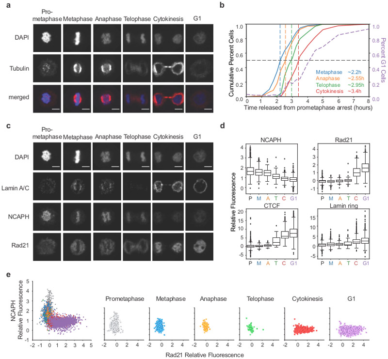
a, Representative images of classification of cell cycle stages based on DAPI staining and tubulin organization (see Methods). Scale bar = 5 μm. b, Cumulative plots of HeLaS3-NCAPH-dTomato cells at different cell cycle stages (left axis) and the percent of cells in G1 (right axis) defined by imaging. At least 400 individual cells were classified for each time point: 0 minutes (n = 405 cells), 30m (n = 520), 60m (n = 780), 90m (n = 669), 105m (n = 638), 120m (n = 613), 135m (n = 601), 150m (n = 812), 165m (n = 533), 180m (n = 507), 195m (n = 650), 210m (n = 607), 240m (n = 1057), 270m (n = 760), 300m (n = 855), 360m (n = 1186), 480m (n = 959). c, Localization of Lamin A/C, NCAPH, and Rad21 during different cell cycle stages shown in panel a. Scale bar = 5 μm. For images showing CTCF localization see Extended Data 8a-b. d, Quantification of NCAPH, Rad21 and CTCF colocalization with chromatin and lamin ring formation at different cell cycle stages (see Methods). P = prometaphase, M = metaphase, A = anaphase, T = telophase, C = cytokinesis, G1 = G1. Box plots represent quartiles of the dataset with a line at the median value, whiskers represent range of the dataset, and diamonds outside of whiskers are outliers. Cell numbers for CTCF plot were P (n = 2099 cells), M (n = 1020), A (n = 199), T (n = 39), C (n = 853), and G1 (n = 2142) (see Extended Data 8a-b). For the other three plots, the corresponding numbers were 1601, 1052, 155, 74, 927, and 2100. e, Quantification of Rad21 and NCAPH colocalization with chromatin in single cells at different cell cycle stages. Left plot represents data from all cells with color indicating cell cycle stage. Right plots represent the data separated into each individual cell cycle stage. Four independent experiments were performed with similar results. Source Data are provided in Source data Fig. 6.
Condensin unloading occurs during telophase while cohesin loading occurs during cytokinesis
The derivative of P(s) plots (Fig. 5b) combined with the cell cycle classification described above (Fig. 6b) indicate that the mitotic loop array is disassembled during telophase. The mitotic loop array is generated by condensins I and II, while interphase loops and TADs are mediated by cohesin15, 16, 26, 28, 40. We determined the kinetics with which condensins dissociate and cohesin associates with chromatin as cells exit mitosis. First, we analyzed condensin binding to chromosomes by microscopy in HeLaS3-NCAPH-dTomato cells classified at different cell cycle stages (Fig. 6c-d). Condensin I is associated with chromosomes until late anaphase. By telophase, most of the condensin I has dissociated. In contrast, very little cohesin is observed on chromosomes up until telophase, but is increasingly colocalized with chromatin during cytokinesis when we also observe the formation of a lamin ring. CTCF is not on chromosomes during early mitosis, but becomes colocalized with chromatin during telophase and the bulk of CTCF binds during cytokinesis (Extended Data 8a-c). These observations confirm that during telophase both condensin and cohesin are depleted from the chromatin. This is illustrated at the single cell level in Figure 6e.
Finally, we determined chromatin association of these complexes directly by purifying chromatin-bound proteins followed by semi-quantitative western blot analysis (Fig. 7a). We quantified the level of chromatin binding for proteins of interest from the western blot and normalized each to the Histone H3 level in the corresponding sample (Fig. 7b). We find that SMC4, a subunit of both condensin I and II, dissociates from chromatin rapidly during telophase. Condensin II (NCAPG2, NCAPD3) showed very similar dissociation kinetics, as did condensin I (NCAPH-dTomato, Extended Data 8d). Cohesin (Rad21) started to associate with chromatin after 3 hours release from prometaphase and continued to load as cells entered and progressed through G1. Chromatin association of CTCF, Lamin A, and elongating RNAPII showed very similar binding kinetics as cohesin. The timing of chromatin association of cohesin and CTCF is consistent with earlier studies19, 32, 33 and with more recent chromatin immunoprecipitation experiments33, 41.
Fig. 7: Chromatin association dynamics of condensins and cohesin during mitotic exit.

a, Western blot analysis of chromatin-associated proteins purified from HeLa S3 cells at different time points after release from prometaphase. b, Quantification of the western blot shown in panel a. Protein levels were normalized to Histone H3 levels from the same samples. c, Summary of cellular and chromosomal events as cells exit mitosis and enter G1. Top: Schematic diagrams indicate the cellular events from prometaphase into late G1. Compartment type is indicated by color: blue = A, orange = B. Red lines represent tubulin and dashed gray lines represent lamina. Bottom: Models of chromosome conformation during early mitosis, telophase, cytokinesis, and interphase. Green bar indicates abundance of condensins I and II on the chromatin at the corresponding cell cycle stages. Yellow bar indicates cohesin abundance on the chromatin at the corresponding cell cycle stages. Unprocessed blots are provided in Source Data as Unprocessed Blots Figure 7. Four independent experiments were performed with similar results. Source Data are provided in Source data Fig. 7.
We conclude that during telophase, most condensin has dissociated from the chromosomes and cohesin association with chromosomes is low. This is consistent with the interpretation of the Hi-C data based on the derivate of P(s) that at this time point there is a transient chromatin folding intermediate with no condensin-mediated loops and only a very low density of cohesin loops. As cells progress through cytokinesis, CTCF and cohesin increasingly load on chromosomes and this continues into G1.
Discussion
We identify telophase as a critical intermediate state between the mitotic and interphase chromosome conformation (Fig. 7c). Hi-C, immunolocalization and chromatin binding assays show loss of condensin binding prior to telophase while CTCF and cohesin start loading during cytokinesis. This intermediate conformation is characterized by the absence of most SMC-driven loops and no or very weak long-range inter-compartment interactions. Given that this intermediate occurs during telophase which lasts approximately 20-25 minutes, the lifetime of this intermediate must be similarly short. Subsequently during cytokinesis, CTCF and cohesin re-load, CTCF-CTCF loops and TAD boundaries are re-established as are compartment domains. While TADs and loops become more prominent rapidly with kinetics faster or equal to G1 entry, long-range compartmentalization occurs slower and continues to increase for several hours after cells have entered G1.
Our data show that key features that define the interphase state, loop anchors and domain boundaries are defined prior to cells entering G1. The fact that TADs and loops form rapidly indicates that the process of loop extrusion is relatively fast, extruding loops of up to several hundreds of kb within 15-30 minutes, consistent with previous studies (1-2 Kb per second on naked DNA42, several Kb per minute during prophase28). In contrast, long-range compartmentalization occurs more slowly during several hours in G1, even though their boundaries and identities are detectable much earlier. This is consistent with cytological observations, which show that LADs are not yet peripherally localized during cytokinesis29. This supports the notion that compartmentalization is mechanistically distinct from TAD and loop formation, and has been proposed to be due to phase segregation11-13, 17, 18, 43. A previous study also showed that compartmentalization occurs during early G130. Our data are in line with very recent studies that independently found that domain and loop anchors are established prior to G1 entry while inter-compartment interactions develop slower41.
The formation of an intermediate folding state during telophase coincides with this condensin-to-cohesin transition. Hi-C data for this state shows that chromosomes are mostly devoid of loops and long-range compartmentalization is minimal. The exponent of P(s) for this intermediate fluctuates around −1 for loci separated by 100 kb up to several Mb. Interpretation of this feature is not straightforward. It could represent the fact that chromosomes are transitioning between two states, with the −1 exponent being the average of the two. Alternatively, and more interestingly, an exponent of ~−1 has been proposed to correspond to a largely unentangled fiber10, 44-46. How could this state be formed? One intriguing possibility is that this is a remnant of the condensin-mediated mitotic loop array that is also not entangled. Continuous loop extrusion by condensin complexes, combined with topoisomerase II activity would lead to decatenation of adjacent loops47. Dissociation of condensin during anaphase would then leave a largely unentangled though still linearly arranged conformation. Subsequent cohesin loading would then initiate the formation of loops again. Although at this time the exact topological state of telophase chromosomes is speculative, our results demonstrate that this transient state represents a key intermediate between the mitotic and interphase genome conformations. Future examination of the molecular and physical properties of this intermediate can not only reveal mechanisms by which cells build the interphase nucleus, but may also lead to better insights into the mitotic state from which it is derived.
Methods
Cell Culture
HeLa S3 CCL-2.2 cells (ATCC CCL-2.2) and HeLaS3-NCAPH-dTomato cells (see below) were cultured in DMEM, high glucose, GlutaMAX™ Supplement with pyruvate (Gibco 10569010) with 10% fetal bovine serum (Gibco 16000044) and 1% PenStrep (Gibco 15140) at 37°C in 5% CO2.
Creation of Stable HeLaS3-NCAPH-dTomato Cell Line
We used pSpCas9(BB)-2A-Puro (PX459) V2.0 [a gift from Feng Zhang (Addgene plasmid # 62988 ; http://n2t.net/addgene:62988 ; RRID:Addgene_62988)] to construct CRISPR/Cas vectors according to the protocol of Ran et al. 48. gRNAs are listed in Supplementary Table 1.
To construct donor plasmids for C-terminal integration of dTomato, plasmids were based on pUC19 and constructed using synthesized DNA and homology arms generated by PCR (primers listed in Supplementary Table 2). Template DNA (genomic DNA from HeLa S3 cells) was amplified using Q5 High-Fidelity DNA Polymerase (New England Biolabs) to generate NCAPH homology arms. gBlock containing dTomato and Blasticidin resistance was synthesized by Integrated DNA Technologies (IDT) (sequence in Supplementary Table 3). Homology arms and gBlocks were cloned into pUC19 by Gibson assembly, using NEBuilder® HiFi DNA Assembly Master Mix (NEB).
To generate stable cell lines, 5 × 10⁶ cells were electroporated with gRNAs and donor plasmid. 24 hours after electroporation, 1 μg/ml puromycin was added. Two days later, 1 ug/mL blasticidin was added for NCAPH-dTomato selection. After 5 days, colonies were picked for further selection in a 96-well plate.
HeLaS3-NCAPH-dTomato clone A6 cell line is available upon request, with an MTA from ATCC. Alternatively, the constructs are available to re-create the cell line in original HeLa S3 cells.
Mitotic Synchronization
All prometaphase synchronization of cells were done by (1) single thymidine treatment to arrest cells in S phase, (2) release into standard media to allow cell recovery and entry into late S, and (3) nocodazole treatment to arrest cells in prometaphase. On Day 1, cells were plated at 4 × 10⁶ cells / 15 cm plate in media containing 2mM thymidine (Sigma T1895). After 24 hours, cells were washed with 1× PBS (Gibco 14190144) and standard media was added back to plates for 3 hours. Cells were then treated with media containing 100 ng/mL nocodazole (Sigma M1404) for 12 hours. Floating mitotic cells were collected and washed in 1× PBS.
Mitotic Release Timecourse
For prometaphase samples, washed mitotic cells were immediately prepared for downstream analysis. Remaining samples were re-cultured in standard media for synchronous release into G1 and collected at indicated times. For early time points, both floating and adherent re-cultured cells were collected for analysis. After 5 hours release from nocodazole, only adherent cells were collected.
Approximately 5 × 10⁶ cells at each time point were fixed in 1% Formaldehyde (Fisher BP531-25) diluted in serum-free DMEM for Hi-C analysis as described in Belaghzal et al. 49. For cell cycle analysis, approximately 1 × 10⁶ cells at each time point were fixed in 86% cold ethanol (Fisher 04-355-222) and stored at −20°C. For chromatin association protein analysis, approximately 5 × 10⁶ cells at each time point were pelleted, flash frozen, and stored at −80°C. Additional samples were collected for fluorescent microscopy. Floating mitotic cells were resuspended in 1.5 mL 4% PFA (EMS 15710) (diluted in 1× PBS), transferred onto a Poly-L-lysine-coated coverslip (Sigma P8920) in a 6 well plate, and spun at 1500xg for 15 min. Cells adherent to coverslips at later time points were fixed in 4% PFA for 15 minutes at 20°C. All coverslips were washed 3× in 1× PBS and stored in 1× PBS at 4°C.
Cell Cycle Analysis
Fixed cells were washed in 1× PBS then resuspended in PBS containing 0.1% NP-40 (MP Biomedicals 0219859680), 0.5 mg/mL RNase A (Roche 10109169001) and 50 ug/mL propidium iodide (Thermo P1304MP). Samples were incubated at 20°C for 30 minutes then analyzed via LSR II or MACSQuant VYB flow cytometry. Data was analyzed using FlowJo v3. Viability gates using forward and side scatter were set on the nonsynchronous sample and applied to all samples within the set. DNA content was plotted as a histogram of the red channel. G1, S, and G2/M gates were set on nonsynchronous sample and applied to all samples within the set to get percentage of cells in each state throughout the time course release from prometaphase arrest. Values plotted for kinetics of G1 entry were normalized such that the maximum number of G1 cells = 1.
Hi-C Protocol
Hi-C was performed as described in Belaghzal et al.49. Briefly, flash-frozen cross-linked cell culture samples were lysed then digested with DpnII at 37°C overnight. Next, the DNA overhanging ends were filled with biotin-14-dATP at 23°C for 4 hours and ligated with T4 DNA ligase at 16°C for 4 hours. DNA was then treated with proteinase K at 65°C overnight to remove crosslinked proteins. Ligation products were purified, fragmented by sonication to an average size of 200 bp, and size selected to fragments 100 - 350 bp. We then performed end repair and dA-tailing and selectively purified biotin tagged DNA using streptavidin beads. Illumina TruSeq adaptors were added to form the final Hi-C ligation products, samples were amplified and PCR primers were removed. Hi-C libraries were then sequenced by PE50 bases on an Illumina HiSeq4000.
Hi-C Data Processing
Hi-C PE50 fastq sequencing files were mapped to hg19 human reference genome using distiller-nf mapping pipeline (https://github.com/mirnylab/distiller-nf). In brief, bwa mem was used to map fastq pairs in a single-side regime (-SP). Aligned reads were classified and deduplicated using pairtools (https://github.com/mirnylab/pairtools), such that uniquely mapped and rescued pairs were retained and duplicate pairs (identical positions and strand orientations) were removed. We refer to such filtered reads as valid pairs. Valid pairs were binned into contact matrices at 10 kb, 20 kb, 40 kb, and 200 kb resolutions using cooler50. Iterative balancing procedure 51 was applied to all matrices, ignoring the first 2 diagonals to avoid short-range ligation artifacts at a given resolution, and bins with low coverage were removed using MADmax filter with default parameters. Resultant “.cool” contact matrices were used in downstream analyses using cooltools (https://github.com/mirnylab/cooltools). For downstream analyses using cworld (https://github.com/dekkerlab/cworld-dekker), contact matrices were converted to “.matrix” using cooltools dump_cworld. For visualization of contact matrices (as in Fig. 1), .matrix files were scaled to 100 × 106 reads using cworld scaleMatrix. Hi-C statistics for each sample are in Supplementary Table 4.
Contact probability (P(s)) plots & derivatives
Cis reads from the valid pairs files were used to calculate the contact frequency (P) as a function of genomic separation (s) (adapted from cooltools). All P(s) curves were normalized for the total number of valid interactions in each data set. Corresponding derivative plots were made from each P(s) plot.
Compartment analysis
Compartment boundaries were identified in cis using eigen vector decomposition on 200 kb binned data with cooltools call-compartments function. A and B compartment identities were assigned by gene density tracks such that the more gene-dense regions were labeled A compartments, and the PC1 sign was positive. Change in compartment type, therefore, occurs at locations where the value of PC1 changes sign. Compartment boundaries were defined at these locations, except for when the sign change occurred within 400 kb of another sign change.
To measure compartmentalization strength, we calculated observed/expected Hi-C matrices for 200 kb binned data, correcting for average distance decay as observed in the P(s) plots (cooltools compute-expected). We then arranged observed/expected matrix bins according to their PC1 values of the replicate 1 Hi-C dataset from cells released from prometaphase for 8 hours. We aggregated the ordered matrices for each chromosome within a dataset then divided the aggregate matrix into 50 bins and plotted, yielding a “saddle plot” (cooltools compute-saddle). Strength of compartmentalization was defined as the ratio of (A-A + B-B) / (A-B + B-A) interactions. Values used for this ratio were determined by calculating the mean value of the 10 bins in each corner of the saddle plot. Values plotted for kinetics of compartment formation were normalized such that strength = 0 in prometaphase cells and the maximum value = 1.
In order to observe compartmentalization at different genomic ranges, we extracted observed/expected Hi-C data at specific distances (0-4 Mb, 4-8 Mb, 8-18 Mb, 18-38 Mb, 38-80 Mb) and made saddle plots. Since less data was used as input for each saddle plot, data was split into 20 bins instead of 50. Overall compartmentalization strength was calculated similar to above except using the mean value of the 9 bins in each corner of the saddle plot. Compartmentalization of individual compartment types was defined as the ratio of (A-A / A-B) or (B-B / A-B), where these values were determined by calculating the mean value of the 9 bins in the specified corner of the saddle plot. All values were normalized and plotted for kinetics the same as above.
TAD analysis
Domain boundaries were identified using insulation analysis on 40 kb binned data with cworld matrix2insulation and locating the minima in each profile (--is 520 kb --ids 320 kb). Domain boundaries were classified as compartment boundaries if they overlapped with the compartment boundaries defined above. All other domain boundaries were assumed to be TAD boundaries.
To measure TAD boundary formation, we aggregated 40 kb binned Hi-C data at domain boundaries identified from the replicate 1 Hi-C dataset from cells released from prometaphase for 8 hours (cworld elementPileUp). Insulation score was calculated by dividing the sum of interactions (with loci up to 40-500 kb away) for each bin within 500 kb of a boundary by the average of all interactions (with loci up to 40-500 kb away) for all binds located within 500 kb of a boundary.
Strength of TAD boundary formation was defined as the depletion of interactions across the boundary pileup, i.e. insulation as above. Boundary strength was calculated by measuring the average interaction of domain boundaries with regions 40-500 kb away (center vertical bin of boundary pileup) and subtracting that value from the average signal in regions immediately flanking the domain boundary (all bins left and right of domain boundary). All calculations were made after removing the bin closest to the diagonal. Values plotted for kinetics of TAD formation were normalized such that strength = 0 in prometaphase cells and the maximum value = 1.
Loop analysis
We used a previously identified set of HeLa S3 looping interactions for this analysis2. This set contains 3,094 total loops and 507 looping interactions are on the structurally intact chromosomes of HeLa S3 cells27. To visualize looping interactions observed, we aggregated 10 or 20 kb binned data at loops larger than 200 kb to avoid the strong signal at the diagonal of the interaction matrix (cworld interactionPileUp).
Strength of loop formation was defined as the enrichment of signal at the looping interactions (center 3×3 pixels at loop position 20 kb binned data) compared to the flanking regions. Strength was calculated by averaging the signal at the looping interaction and subtracting the average signal outside. Values plotted for kinetics of loop formation were normalized such that strength = 0 in prometaphase cells and the maximum value = 1.
In order to observe formation of looping interactions at all loops sizes, we aggregated observed/expected Hi-C matrices for 20 kb binned Hi-C data at sites of looping interactions. Using the observed/expected matrices corrects for distance decay and removes the overwhelming signal close to the diagonal, allowing us to observe smaller loops than in the observed Hi-C matrices.
Simulated Hi-C mixture datasets
We generated simulated Hi-C datasets for each replicate time course experiment. For each replicate the following protocol was used to randomly mix reads from prometaphase Hi-C datasets (t = 0 hours) with random Hi-C data reads from the sample having the highest percentage of G1 cells in the respective time course (t = 8 hours for replicates 1 and 2, t = 6 hours for replicate 3). Mixing ratios were determined based on cell cycle analysis of the same time course replicate, such that x% prometaphase reads + 1-x% G1 reads was representative of the experimental FACs profile observed at each time point.
First, in order to properly compare samples, all valid pair files within a single Hi-C timecourse dataset were randomly down-sampled to the lowest number of uniquely mapped reads within that timecourse dataset. Next, the down-sampled valid pairs for experimental prometaphase (t = 0 hours) and experimental G1 (t = 6 or 8 hours) were randomly sampled to yield the correct ratio of experimental cells at each time point and the same number of total reads as the down-sampled valid pairs files. This step was repeated 25 times, resulting in 25 simulated valid pairs files with the same number of reads for each time point in each replicate. P(s) plots for simulated Hi-C data represent the average P(s) for 25 replicate valid pair simulations. For all other analyses, valid pairs files were binned and balanced (as above) into “.cool” contact matrices and the 25 replicates from the same simulated ratios were combined using cooler merge.
Microscopy
Immunofluorescence staining
Immunofluorescence staining was performed at room temperature. Fixed cells were permeabilized with 0.1% triton (Sigma T8787) in 1× PBS for 10 minutes. Cells were blocked with 3% BSA (Sigma A7906) in 0.1% triton/PBS for 1 hour. Cells were incubated with primary antibody diluted in the blocking buffer for 2 hours [Lamin A/C (636) mouse mAb (1:800, SantaCruz sc-7292 lot C2219), Rad21 rabbit pAb (1:1000, abcam ab154769, lot GR3224138-10), CTCF rabbit pAb (1:800, Cell Signaling 2899, lot 2)]. Cells were washed with 0.1% triton/PBS 3 × 5 minutes. Cells were incubated with secondary antibodies [goat anti-rabbit IgG H&L Alexa Fluor 488 (1:1000, abcam ab15007, lot GR3225678-1), goat anti-mouse IgG H&L Alexa Fluor 700 (1:1000, invitrogen A-21036, lot 2084419)] diluted in the blocking buffer and conjugated tubulin antibody [anti-tubulin (YOL1/34)-AlexaFluor647, rat mAb, 1:100, abcam ab195884, lot GR281429-4] for 1 hour in the dark.
Cells were washed with 0.1% triton/PBS 1 × 5 minutes and then washed with 1× PBS 3 × 5 minutes. Coverslips were mounted to slides using ProLong Diamond Antifade Mountant with DAPI (Invitrogen P36962). For image acquisition, we used a Leica TCS SP5- II confocal microscope with 405 nm, 488 nm, 561 nm, and 633 nm lasers. Imaging we performed using a Leica HPX PL APO 63X/1.40-0.6 oil immersion objective with standard PMTs. Images were acquired using Leica LAS AF.
Cell Cycle Classification
Images were split into individual tiffs by channel and analyzed using Cell Profiler 3.1.8 and Cell Profiler Analyst 2.2.152, 53. For each image, we identified nuclei as primary objects in the DAPI channel (‘DNA’). We then used propagation from each ‘DNA’ object to look for secondary objects in the tubulin channel (‘tubulin’). At this point, blinded tiffs of each individual cell with DAPI and tubulin staining could be isolated. Cells were manually classified into either prometaphase, metaphase, anaphase, telophase, cytokinesis, or G1 based on the morphology of DNA and tubulin. Prometaphase cells were defined as cells with condensed chromosomes and disrupted tubulin structure due to the microtubule inhibitor used for prometaphase arrest. Cells classified as metaphase had a single axis of DAPI staining with tubulin aligned on each side. Anaphase cells had tubulin on each side of the DAPI axis but must have had two distinct DAPI clusters representing the separation of two genomic copies. Telophase classification was characterized by the presence of tubulin only between the two DAPI populations and no longer on the ends. When the tubulin signal was compressed between the two DAPI clusters, we classified those as cells undergoing cytokinesis. Finally, all cells with decondensed chromatin and no nuclear tubulin were classified as G1 cells. Post-classification, cells were un-blinded and matched back to the corresponding image to allow for the measurement of cumulative counts for each cell cycle phase and the percentage of cells entering G1 over the time course. A total of 13,470 cells were classified in this study.
Protein Localization
Cell Profiler was also used to measure the localization of NCAPH-dTomato, Rad21, CTCF, and Lamin A/C. In addition to the primary nuclei objects (‘DNA’) and the secondary objects (‘tubulin’) defined above (see Cell Cycle Classification), we created a tertiary object as the region between the primary and secondary objects (‘cytoplasm’). We calculated enrichment of NCAPH, Rad21, and CTCF co-localizing with the chromatin by measuring the mean fluorescence intensity (MFI) of each protein overlapping with the ‘DNA’ object and subtracting the MFI of each protein overlapping with the ‘cytoplasm’ object.
To measure the formation of a lamin ring, we shrunk the ‘DNA’ object and subtracted this region from the ‘DNA’ original object to create a new object (‘lamin’) at the inside edge of the ‘DNA’ where we observed lamin ring presence in nonsynchronous cells. Next, we expanded the ‘DNA’ object and subtracted the original ‘DNA’ object to create a new object (‘LamCyto’) just outside of the ‘lamin’ object. We were able to quantify the presence of a lamin ring by subtracting the MFI of lamin fluorescence in ‘LamCyto’ region from the MFI of lamin in the ‘lamin’ region. This enriched for the signal of a lamin ring, therefore, higher values correlated with the presence of a lamin ring structure at the edge of the chromatin.
Chromatin association
Fractionation protocol
Flash-frozen cell pellets from each time point of the mitotic release time course were thawed and resuspended with lysis buffer (50 mM Tris-HCl, pH 8.0, 100 mM NaCl, 1% NP-40, 1 mM DTT, 1× Halt protease inhibitor cocktail (Thermo 78430)). Samples in lysis buffer were incubated on ice for 20 minutes and then spun at 13,000 × g for 10 minutes at 4°C. The supernatant (cytoplasmic fraction) was collected and the pellet was resuspended in nuclei buffer (10 mM PIPES, pH 7.4, 10 mM KCl, 2 mM MgCl2, 0.1% NP-40, 1 mM DTT, 1× protease inhibitor) with 0.25% triton. Samples were incubated on ice for 10 minutes and then spun at 10,000 × g for 5 minutes at 4°C. The supernatant (nucleoplasmic fraction) was collected and the pellet (chromatin fraction) was resuspended in nuclei buffer with 20% glycerol. The chromatin fraction was then sonicated to shear the DNA using a Covaris instrument with the following parameters: 10% duty cycle, intensity 5, 200 cycles/burst, frequency sweeping, continuous degassing, 240 second process time, 4 cycles. Final chromatin-bound protein samples were stored at −20°C.
Western Blots
The volume for approximately the same number of cells for each sample across the mitotic release time course was loaded in each lane of a 4-12% bis-tris protein gel (Biorad 3450125) and separated in 1× MES running buffer (Biorad 1610789). Proteins were transferred to nitrocellulose membranes (Bio-Rad 1620112) at 30 V for 1.5 hours in 1× transfer buffer (Thermo 35040). Membranes were blocked with 4% milk in PBS-T (1× PBS + 0.1% tween) for 1 hour at room temperature. Membranes were then incubated with specified primary antibody diluted 1:1000 in 4% milk/PBS-T overnight at 4°C [Histone H3 (ab1791), Rad21 (ab154769), RFP (cross-reacts with dTomato for NCAPH-dTomato, Rockland 600-401-379), SMC2 (ab10412), SMC4 (ab17958), NCAPD3 (ab70349), NCAPG2 (ab70350), Lamin A (ab26300), CTCF (Cell Signaling 2899), RNA polymerase II CTD repeat phospho S2 (ab5095)]. Membranes were washed with PBS-T 3 × 10 minutes at room temperature, then incubated with secondary antibody (anti-rabbit IgG HRP-linked, Cell Signaling 7074) diluted 1:4000 in 4% milk/PBS-T for 2 hours at room temperature. Membranes were washed with PBS-T 3 × 10 minutes. Membranes were developed and imaged using SuperSignal West Dura Extended Duration Substrate (Thermo 34076) and Bio-Rad ChemiDoc.
Quantification
Band intensity for each protein was quantified using Image Lab 5.2.1. Intensities for each lane were normalized by background intensity of an equal sized area in the same lane. All protein quantifications were normalized to the Histone H3 levels for the same time course samples.
Statistics and Reproducibility
No statistical methods were used to predetermine sample size. Three replicate Hi-C time courses were performed independently with similar results. For imaging experiments, the number of cells analyzed was the maximum experimentally feasible.
Code Availability
Code for Hi-C analyses are available at the following links: distiller-nf (https://github.com/mirnylab/distiller-nf), pairtools (https://github.com/mirnylab/pairtools), cooltools (https://github.com/mirnylab/cooltools), cworld (https://github.com/dekkerlab/cworld-dekker).
Data Availability
Sequencing data generated in this study have been deposited in the Gene Expression Omnibus (GEO) repository under accession GSE133462. Dataset titled “R1” refers to replicate 1 which is used in Figures 1-5, and Extended Data 1-5. Dataset titled “R2” refers to replicate 2 which is used in Figure 2, and Extended Data 1 and 6. Dataset titled “R3” refers to replicate 3 which is used in Figure 2, and Extended Data 1 and 7. Data from this publication can also be accessed in the 4DN Data Portal with link https://data.4dnucleome.org/abramo_et_al_2019. All other data supporting the findings of this study are available from the corresponding author on reasonable request.
Supplementary Material
Extended Data
Extended Data Fig. 1. Cell cycle analysis of mitotic exit time courses.

a, FACS analysis of nonsynchronous and prometaphase-arrested cultures and of cultures at different time points after release from prometaphase-arrest in time course replicate 1. Percentages in the upper right corner represent the number of cells with a G1 DNA content. b-d, Quantification of the fraction of cells in G1 at each time point from time course replicate 1 normalized to t = 8 hours (b), time course replicate 2 normalized to t = 8 hours (c), and time course replicate 3 normalized to a G1 maximum assumed to be 80% (d). Three independent experiments were performed with similar results. Source Data are provided in Source data Extended Data Fig. 1.
Extended Data Fig. 2. Compartment analysis for time course replicate 1.

a, Principal component 1 (PC1) along Chromosome 14 for Hi-C data obtained from cells at different time points after release from prometaphase. Principal component analysis was performed on Hi-C data binned at 200 kb resolution. PC1 detects A and B compartments starting at t = 3 hours. Lower left corner represents Pearson correlation value of each track compared to nonsynchronous PC1. b, Principal component 3 (PC3) along Chromosome 14 for Hi-C data obtained from cells at different time points after release from prometaphase. Principal component analysis was performed on Hi-C data binned at 200 kb resolution. PC3 detects some A and B compartments starting at t = 2.75 hours, but at later time points, PC1 captures compartments. Lower left corner represents Pearson correlation value of each track compared to nonsynchronous PC1. Three independent experiments were performed with similar results.
Extended Data Fig. 3. TAD and compartment domain boundaries form with similar kinetics.

a, Aggregate Hi-C data binned at 40 kb resolution at domain boundaries (top = all 724 boundaries, middle = 657 TAD boundaries, bottom = 67 compartment boundaries) at different time points after release from prometaphase. b, Average insulation profile across averaged domain boundaries shown in panel a (left = TAD boundaries, right = compartment boundaries) for different time points. c, Normalized strength for domain boundaries as a function of time after release from prometaphase. The strength for each of these features was set at 1 for the 8 hour time point. TAD boundaries and compartment boundaries form with similar kinetics. Three independent replicate experiments yielded similar results. Source Data are provided in Source Data Extended Data Fig. 3.
Extended Data Fig. 4. Compartment analysis for chromosome 14.

a, Saddle plots of Hi-C data for chromosome 14 binned at 200 kb resolution for different time points and split into genomic distance bands, as shown in gray in the first row. b, Normalized compartmentalization strength of different genomic distances as a function of time and split by interaction type (A-A, B-B, A-B). c, Normalized compartmentalization strength of interaction types as a function of time and split by genomic distance. Three independent experiments were performed with similar results. Source Data are provided in Source data Extended Data Fig. 4.
Extended Data Fig. 5. Kinetics of loop formation for loops of different size.

Loops were grouped according to size: a, loops less than or equal to 125 kb, b, loops greater than 125 kb and less than or equal to 200 kb, c, loops greater than 200 kb and less than or equal to 325 kb, d, loops greater than 325 kb. For each panel, top row: log2(observed/expected) Hi-C data for experimental time course, middle row: log2(observed/expected) Hi-C data for simulated time course, bottom row: the difference between experimental and simulated Hi-C data. Kinetics of loop formation is similar for all loop sizes. Three independent experiments were performed with similar results.
Extended Data Fig. 6. Analysis of time course replicate 2.

a, Aggregated Hi-C data binned at 20 kb resolution at chromatin loops at different time points. Top row: Experimental Hi-C data. Middle row: Simulated Hi-C data. Bottom row: The difference between experimental and simulated Hi-C data. Loops are more prominent in experimental Hi-C data than in the simulated data between 3 and 4.5 hours. This analysis included loops larger than 200 kb to avoid the strong signal at the diagonal of the interaction matrix. Simulations were performed with experimental data from this time course (mixing Hi-C data for t = 0 and t = 8 hours). b, Aggregate Hi-C data binned at 40 kb resolution at TAD boundaries for different time points. Top row: Experimental Hi-C data. Middle row: Simulated Hi-C data. Bottom row: The difference between experimental and simulated Hi-C data. Insulation strength is stronger in experimental Hi-C data than in simulated Hi-C data at t = 3.5 and t = 4.5 hours. c, Saddle plots of Hi-C data binned at 200 kb resolution for different time points. Top row: Experimental Hi-C data. Middle row: Simulated Hi-C data. Bottom row: The difference between experimental and simulated Hi-C data. Compartmentalization is weaker in experimental Hi-C than in simulated Hi-C data as illustrated by the fact that A-B interactions are less depleted in the experimental data (upper right and lower left corner of saddle plots). d, Derivative from P(s) plots. Black lines represent the derivative of P(s) for experimental Hi-C data and the dashed green lines represent the derivative of P(s) for the simulated Hi-C datasets for corresponding time points. Three independent experiments were performed with similar results.
Extended Data Fig. 7. Analysis of time course replicate 3.

a, Aggregated Hi-C data binned at 20 kb resolution at chromatin loops at different time points. Top row: Experimental Hi-C data. Middle row: Simulated Hi-C data. Bottom row: The difference between experimental and simulated Hi-C data. Loops are more prominent in experimental Hi-C data than in the simulated data between 3.25 and 4 hours. This analysis included loops larger than 200 kb to avoid the strong signal at the diagonal of the interaction matrix. Simulations were performed with experimental data from this time course (mixing Hi-C data for t = 0 and t = 6 hours). b, Aggregate Hi-C data binned at 40 kb resolution at TAD boundaries for different time points. Top row: Experimental Hi-C data. Middle row: Simulated Hi-C data. Bottom row: The difference between experimental and simulated Hi-C data. Insulation strength is stronger in experimental Hi-C data than in simulated Hi-C data at t = 3.25 and t = 4 hours. c, Saddle plots of Hi-C data binned at 200 kb resolution for different time points. Top row: Experimental Hi-C data. Middle row: Simulated Hi-C data. Bottom row: The difference between experimental and simulated Hi-C data. Compartmentalization is weaker in experimental Hi-C than in simulated Hi-C data as illustrated by the fact that A-B interactions are less depleted in the experimental data (upper right and lower left corner of saddle plots). d, Derivative from P(s) plots. Black lines represent the derivative of P(s) for experimental Hi-C data and the dashed green lines represent the derivative of P(s) for the simulated Hi-C datasets for corresponding time points. Three independent experiments were performed with similar results.
Extended Data Fig. 8. Chromatin association dynamics of CTCF, condensin, and cohesion.

a, Classification of cell cycle stages based on DAPI staining and tubulin organization. Scale bar = 5μm. b, Localization of Lamin A/C, NCAPH, and CTCF during different cell cycle stages shown in panel a. Scale bar = 5μm. c, Quantification of CTCF and NCAPH colocalization with chromatin in single cells at different cell cycle stages. Left plot represents data from all cells with color indicating cell cycle stage. Right plots represent the data separated into each individual cell cycle stage. d, Top: Western blot analysis of chromatin-associated proteins purified from HeLaS3-NCAPH-dTomato cells at different time points after release from prometaphase. Bottom: Quantification of the western blot shown above. NCAPH and Rad21 were analyzed on the same gel. The samples for Histone H3 analysis were run on another gel. Four independent experiments were performed with similar results. Source Data for microscopy are provided in Source data Fig. 7. Unprocessed blots are provided in Source data Extended Data Fig. 8.
Acknowledgements
We thank Christina Baer from the UMass SCOPE Imaging Core for advice on imaging and help with the classification pipeline on CellProfiler. We thank members of the Dekker lab and Mirny lab for discussions. We acknowledge support from the National Institutes of Health Common Fund 4D Nucleome Program (DK107980), and the National Human Genome Research Institute (HG003143). J.D is an investigator of the Howard Hughes Medical Institute.
Footnotes
Competing Interests
The authors declare no competing interests.
References
- 1.Fudenberg G, Abdennur N, Imakaev M, Goloborodko A & Mirny LA Emerging Evidence of Chromosome Folding by Loop Extrusion. Cold Spring Harb Symp Quant Biol 82, 45–55 (2017). [DOI] [PMC free article] [PubMed] [Google Scholar]
- 2.Rao SSP et al. A 3D map of the human genome at kilobase resolution reveals principles of chromatin looping. Cell 159, 1665–1680 (2014). [DOI] [PMC free article] [PubMed] [Google Scholar]
- 3.de Wit E et al. CTCF Binding Polarity Determines Chromatin Looping. Mol Cell. 60, 676–684 (2015). [DOI] [PubMed] [Google Scholar]
- 4.Guo Y et al. CRISPR Inversion of CTCF Sites Alters Genome Topology and Enhancer/Promoter Function. Cell 162, 900–910 (2015). [DOI] [PMC free article] [PubMed] [Google Scholar]
- 5.Vietri Rudan M et al. Comparative Hi-C reveals that CTCF underlies evolution of chromosomal domain architecture. Cell Rep. 10, 1297–1309 (2015). [DOI] [PMC free article] [PubMed] [Google Scholar]
- 6.Sanborn AL et al. Chromatin extrusion explains key features of loop and domain formation in wild-type and engineered genomes. Proc Natl Acad Sci U S A. 112, E6456–6465 (2015). [DOI] [PMC free article] [PubMed] [Google Scholar]
- 7.Fudenberg G et al. Formation of chromosomal domains by loop extrusion. Cell Rep. 15, 2038–2049 (2016). [DOI] [PMC free article] [PubMed] [Google Scholar]
- 8.Nora EP et al. Spatial partitioning of the regulatory landscape of the X-inactivation centre. Nature 485, 381–385 (2012). [DOI] [PMC free article] [PubMed] [Google Scholar]
- 9.Dixon JR et al. Topological domains in mammalian genomes identified by analysis of chromatin interactions. Nature 485, 376–380 (2012). [DOI] [PMC free article] [PubMed] [Google Scholar]
- 10.Lieberman-Aiden E et al. Comprehensive mapping of long-range interactions reveals folding principles of the human genome. Science 326, 289–293 (2009). [DOI] [PMC free article] [PubMed] [Google Scholar]
- 11.Di Pierro M, Zhang B, Aiden EL, Wolynes PG & Onuchic JN Transferable model for chromosome architecture. Proc Natl Acad Sci U S A 113, 12168–12173 (2016). [DOI] [PMC free article] [PubMed] [Google Scholar]
- 12.Erdel F & Rippe K Formation of Chromatin Subcompartments by Phase Separation. Biophys J 114, 2262–2270 (2018). [DOI] [PMC free article] [PubMed] [Google Scholar]
- 13.Michieletto D, Orlandini E & Marenduzzo D Polymer model with epigenetic recoloring reveals a pathway for the de novo establishment and 3D organization of chromatin domains. Phys. Rev. X 6, 041047 (2016). [Google Scholar]
- 14.Nora EP et al. Targeted Degradation of CTCF Decouples Local Insulation of Chromosome Domains from Genomic Compartmentalization. Cell 169, 930–944 e922 (2017). [DOI] [PMC free article] [PubMed] [Google Scholar]
- 15.Schwarzer W et al. Two independent modes of chromatin organization revealed by cohesin removal. Nature 551, 51–56 (2017). [DOI] [PMC free article] [PubMed] [Google Scholar]
- 16.Rao SSP et al. Cohesin Loss Eliminates All Loop Domains. Cell 171, 305–320 e324 (2017). [DOI] [PMC free article] [PubMed] [Google Scholar]
- 17.Nuebler J, Fudenberg G, Imakaev M, Abdennur N & Mirny LA Chromatin organization by an interplay of loop extrusion and compartmental segregation. Proc Natl Acad Sci U S A 115, E6697–E6706 (2018). [DOI] [PMC free article] [PubMed] [Google Scholar]
- 18.Falk M et al. Heterochromatin drives organization of conventional and inverted nuclei. Nature In 570, 395–399 (2019). [DOI] [PMC free article] [PubMed] [Google Scholar]
- 19.Sumara I, Vorlaufer E, Gieffers C, Peters BH & Peters JM Characterization of vertebrate cohesin complexes and their regulation in prophase. J Cell Sci 151, 749–762 (2000). [DOI] [PMC free article] [PubMed] [Google Scholar]
- 20.Losada A, Hirano M & Hirano T Cohesin release is required for sister chromatid resolution, but not for condensin-mediated compaction, at the onset of mitosis. Genes Dev 16, 3004–3016 (2002). [DOI] [PMC free article] [PubMed] [Google Scholar]
- 21.Paulson JR & Laemmli UK The structure of histone-depleted metaphase chromosomes. Cell. 12, 817–828 (1977). [DOI] [PubMed] [Google Scholar]
- 22.Marsden MP & Laemmli UK Metaphase chromosome structure: evidence for a radial loop model. Cell. 17, 849–858 (1979). [DOI] [PubMed] [Google Scholar]
- 23.Hirano T & Mitchison TJ A heterodimeric coiled-coil protein required for mitotic chromosome condensation in vitro. Cell 79, 449–458 (1994). [DOI] [PubMed] [Google Scholar]
- 24.Strunnikov AV, Hogan E & Koshland D SMC2, a Saccharomyces cerevisiae gene essential for chromosome segregation and condensation, defines a subgroup within the SMC family. Genes Dev. 9, 587–599 (1995). [DOI] [PubMed] [Google Scholar]
- 25.Hirano T, Kobayashi R & Hirano M Condensins, chromosome condensation protein complexes containing XCAP-C, XCAP-E and a Xenopus homolog of the Drosophila Barren protein. Cell 89, 511–521 (1997). [DOI] [PubMed] [Google Scholar]
- 26.Ono T et al. Differential contributions of condensin I and condensin II to mitotic chromosome architecture in vertebrate cells. Cell 115, 109–121 (2003). [DOI] [PubMed] [Google Scholar]
- 27.Naumova N et al. Organization of the mitotic chromosome. Science 342, 948–953 (2013). [DOI] [PMC free article] [PubMed] [Google Scholar]
- 28.Gibcus JH et al. A pathway for mitotic chromosome formation. Science 359 (2018). [DOI] [PMC free article] [PubMed] [Google Scholar]
- 29.Kind J et al. Single-cell dynamics of genome-nuclear lamina interactions. Cell 153, 178–192 (2013). [DOI] [PubMed] [Google Scholar]
- 30.Dileep V et al. Topologically associating domains and their long-range contacts are established during early G1 coincident with the establishment of the replication-timing program. Genome Res 25, 1104–1113 (2015). [DOI] [PMC free article] [PubMed] [Google Scholar]
- 31.Walther N et al. A quantitative map of human Condensins provides new insights into mitotic chromosome architecture. J Cell Biol 217, 2309–2328 (2018). [DOI] [PMC free article] [PubMed] [Google Scholar]
- 32.Darwiche N, Freeman LA & Strunnikov A Characterization of the components of the putative mammalian sister chromatid cohesion complex. Gene 233, 39–47 (1999). [DOI] [PMC free article] [PubMed] [Google Scholar]
- 33.Cai Y et al. Experimental and computational framework for a dynamic protein atlas of human cell division. Nature 561, 411–415 (2018). [DOI] [PMC free article] [PubMed] [Google Scholar]
- 34.Crane E et al. Condensin-driven remodeling of X-chromosome topology during dosage compensation. Nature doi: 10.1038/nature14450 (2015). [DOI] [PMC free article] [PubMed] [Google Scholar]
- 35.Lajoie BR, Dekker J & Kaplan N The Hitchhiker's guide to Hi-C analysis: Practical guidelines. Methods 72, 65–75 (2015). [DOI] [PMC free article] [PubMed] [Google Scholar]
- 36.Oomen ME, Hansen AS, Liu Y, Darzacq X & Dekker J CTCF sites display cell cycle-dependent dynamics in factor binding and nucleosome positioning. Genome Res 29, 236–249 (2019). [DOI] [PMC free article] [PubMed] [Google Scholar]
- 37.Dekker J, Rippe K, Dekker M & Kleckner N Capturing Chromosome Conformation. Science 295, 1306–1311 (2002). [DOI] [PubMed] [Google Scholar]
- 38.Gassler J et al. A mechanism of cohesin-dependent loop extrusion organizes zygotic genome architecture. EMBO J 36, 3600–3618 (2017). [DOI] [PMC free article] [PubMed] [Google Scholar]
- 39.Patel L et al. Dynamic reorganization of the genome shapes the recombination landscape in meiotic prophase. Nat Struct Mol Biol 26, 164–174 (2019). [DOI] [PMC free article] [PubMed] [Google Scholar]
- 40.Hirano T Condensin-Based Chromosome Organization from Bacteria to Vertebrates. Cell 164, 847–857 (2016). [DOI] [PubMed] [Google Scholar]
- 41.Zhang H et al. Re-configuration of chromatin structure during the mitosis-G1 phase transition. BioRxiv doi: 10.1101/604355 (2019). [DOI] [PMC free article] [PubMed] [Google Scholar]
- 42.Ganji M et al. Real-time imaging of DNA loop extrusion by condensin. Science 360, 102–105 (2018). [DOI] [PMC free article] [PubMed] [Google Scholar]
- 43.Jost D, Carrivain P, Cavalli G & Vaillant C Modeling epigenome folding: formation and dynamics of topologically associated chromatin domains. Nucleic Acids Res 42, 9553–9561 (2014). [DOI] [PMC free article] [PubMed] [Google Scholar]
- 44.Grosberg AY, Nechaev SK & Shakhnovich EI The role of topological constraints in the kinetics of collapse of macromolecules. J. Phys. 49, 2095–2100 (1988). [Google Scholar]
- 45.Grosberg AY, Rabin Y, Havlin S & Neer A Crumpled globule model of the three-dimensional structure of DNA. Europhys. Lett. 23, 373–378 (1993). [Google Scholar]
- 46.Mirny LA The fractal globule as a model of chromatin architecture in the cell. Chromosome Res. 19, 37–51 (2011). [DOI] [PMC free article] [PubMed] [Google Scholar]
- 47.Goloborodko A, Imakaev MV, Marko JF & Mirny L Compaction and segregation of sister chromatids via active loop extrusion. Elife 5 (2016). [DOI] [PMC free article] [PubMed] [Google Scholar]
- 48.Ran FA et al. Genome engineering using the CRISPR-Cas9 system. Nat Protoc 8, 2281–2308 (2013). [DOI] [PMC free article] [PubMed] [Google Scholar]
- 49.Belaghzal H, Dekker J & Gibcus JH Hi-C 2.0: An optimized Hi-C procedure for high-resolution genome-wide mapping of chromosome conformation. Methods 123, 56–65 (2017). [DOI] [PMC free article] [PubMed] [Google Scholar]
- 50.Abdennur N & Mirny LA Cooler: scalable storage for Hi-C data and ther genomically-labelled arrays. BioRxiv doi: 10.1101/557660 (2019). [DOI] [PMC free article] [PubMed] [Google Scholar]
- 51.Imakaev M et al. Iterative correction of Hi-C data reveals hallmarks of chromosome organization. Nature Methods 9, 999–1003 (2012). [DOI] [PMC free article] [PubMed] [Google Scholar]
- 52.Carpenter AE et al. CellProfiler: image analysis software for identifying and quantifying cell phenotypes. Genome Biol 7, R100 (2006). [DOI] [PMC free article] [PubMed] [Google Scholar]
- 53.Jones TR et al. CellProfiler Analyst: data exploration and analysis software for complex image-based screens. BMC Bioinformatics 9, 482 (2008). [DOI] [PMC free article] [PubMed] [Google Scholar]
Associated Data
This section collects any data citations, data availability statements, or supplementary materials included in this article.
Supplementary Materials
Data Availability Statement
Sequencing data generated in this study have been deposited in the Gene Expression Omnibus (GEO) repository under accession GSE133462. Dataset titled “R1” refers to replicate 1 which is used in Figures 1-5, and Extended Data 1-5. Dataset titled “R2” refers to replicate 2 which is used in Figure 2, and Extended Data 1 and 6. Dataset titled “R3” refers to replicate 3 which is used in Figure 2, and Extended Data 1 and 7. Data from this publication can also be accessed in the 4DN Data Portal with link https://data.4dnucleome.org/abramo_et_al_2019. All other data supporting the findings of this study are available from the corresponding author on reasonable request.