Abstract
Understanding cell geometric and mechanical properties is crucial to understanding how cells sense and respond to their local environment. Moreover, changes to cell mechanical properties under varied micro-environmental conditions can both influence and indicate fundamental changes to cell behavior. Atomic Force Microscopy (AFM) is a well established, powerful tool to capture geometric and mechanical properties of cells. We have previously demonstrated substantial functional and behavioral differences between aortic and pulmonary valve interstitial cells (VIC) using AFM and subsequent models of VIC mechanical response. In the present work, we extend these studies by demonstrating that to best interpret the spatially distributed AFM data, the use of spatial statistics is required. Spatial statistics includes formal techniques to analyze spatially distributed data, and has been used successfully in the analysis of geographic data. Thus, spatially mapped AFM studies of cell geometry and mechanics are analogous to more traditional forms of geospatial data. We are able to compare the spatial autocorrelation of stiffness in aortic and pulmonary valve interstitial cells, and more accurately capture cell geometry from height recordings. Specifically, we showed that pulmonary valve interstitial cells display higher levels of spatial autocorrelation of stiffness than aortic valve interstitial cells. This suggests that aortic VICs form different stress fiber structures than their pulmonary counterparts, in addition to being more highly expressed and stiffer on average. Thus, the addition of spatial statistics can contribute to our fundamental understanding of the differences between cell types. Moving forward, we anticipate that this work will be meaningful to enhance direct analysis of experimental data and for constructing high fidelity computational of VICs and other cell models.
Keywords: atomic force microscopy, cell mechanics, cell modeling
1. Introduction
Cell mechanical and geometric properties play an important role in how cells sense and interact with their surrounding environment (Luo et al., 2016). Quantifying these properties is crucial for understanding the specific roles of mechanical forces in biological tissues (Haase and Pelling, 2015; Lejeune and Linder, 2017; Rigato et al., 2015), including quantifying variation between different cell types(Cross et al., 2008). For example, in the mechanically demanding heart valve tissue micro-environment, valve interstitial cells (VICs) respond to mechanical stimuli due to altered hemodynamic conditions and subsequently contribute to tissue remodeling (Ayoub et al., 2011, 2017). Therefore, understanding how VICs feel their surroundings is crucial for robustly predicting how heart valve surgical interventions can lead to tissue remodeling (Rego and Sacks, 2017; Sacks et al., 2017), and measuring mechanobiological variations between VICs derived from different sources provides insight into characteristic physiological and pathological changes (Merryman et al., 2006, 2007).
Atomic force microscopy (AFM) is a popular and well established tool to quantify both cell topography and intrinsic cell mechanical properties on two-dimensional substrates (Gavara, 2017). To measure mechanical properties, an AFM probe is used for micro-indentation. The cantilever tip indents the cell at discrete grid points and the force response curve for each indentation is used to approximate the value of local cell stiffness, reported as apparent elastic modulus (Merryman et al., 2007; Mathur et al., 2001). To measure cell topography, the scanning probe is dragged over the surface of the cell and height is recorded at densely spaced points along the path of the probe (Merryman et al., 2007; Radmacher et al., 1992). Typically, data from these experiments is presented visually, as cell height and stiffness maps, and quantitatively, through the mean and standard deviations of these measured values (Yeow et al., 2017). Furthermore, cell indentation by AFM has been modeled extensively (Nguyen et al., 2016). Our group has used AFM in the study of VICs, both directly (Merryman et al., 2007), and in simulations (Sakamoto et al., 2016, 2017).
As AFM data is recorded at multiple points in space, it is natural to turn to the field of spatial statistics to analyze, and ultimately model, the resulting spatially distributed data. Spatial statistics is specifically intended to handle data where the assumption of independence among observations is violated (Ripley, 2005). For example, spatial statistics is used to characterizing spatial autocorrelation, the co-variation of properties within space, and detect patterns and anomalies in spatially distributed data (Goodchild, 1986). The field of spatial statistics also covers methods for more sophisticated interpolation techniques to make enhanced predictions at unmeasured locations (Stein, 1999). The most common application of spatial statistics is in analyzing geographic data and creating geographic models, where specialized statistical analysis software packages are used in both research and industry (Steiniger and Hunter, 2012). Though spatial statistics is a natural toolset for handling spatially distributed data, such as that generated by AFM studies of biological materials, to the authors’ knowledge, this application has yet to be explored in detail.
In the present work, we show how the toolset of spatial statistics can be meaningfully applied to the problem of analyzing the spatially mapped data from AFM cell studies. Specifically, we introduce three example methods from the spatial statistics literature: single variable measurements of spatial autocorrelation, empirical semivariograms, and Gaussian process regression. Then, we show the results of applying these methods to AFM studies of aortic valve interstitial cells (AVICs) and pulmonary valve interstitial cells (PVICs). Critically, these methods quantitatively reveal different spatial autocorrelation behaviors in AVIC and PVIC stiffness. These results suggest that differences between AVIC and PVIC stiffness are a result of both intrinsic stress-fiber stiffness, and also how sub-cellular components are spatially distributed within the cell. The results of this study and the methods presented can also be extended to the general AFM studies of cell mechanics.
2. Methods
In this section, we briefly introduce three non-standard methods to spatially interpret AFM data. The first two methods that we introduce, computing Moran’s I and plotting an empirical semivariogram, are useful for understanding spatial autocorrelation in experimentally recorded data. Essentially, they show how similar the measured values are at spatially close locations. The third method that we introduce, Gaussian process regression, is a pragmatic strategy for interpolating spatial data. If statistically significant spatial autocorrelation is detection with the first two methods, then Gaussian process regression can be used to predict unseen values y* at unsampled locations x* in order to construct robust models of cells with heterogeneous material properties.
2.1. Experimental data source
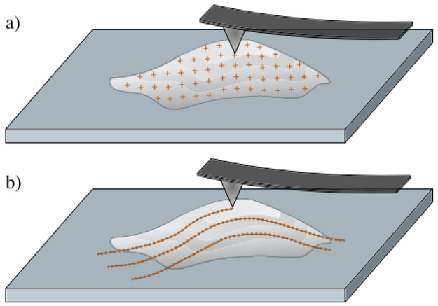
The AFM data for this work was taken from (Merryman et al., 2007), in which information on the experimental methods has been extensively detailed. Briefly, porcine AVICs and PVICs were isolated from the same animal. The AV and PV leaflets were dissected, leaflet surfaces were scraped to remove endothelial cells, and the leaflets were digested and strained to isolate the VICs. Both populations were plated separately in 250 ml culture flasks in complete media. A monolayer of seeded VICs from each valve type were structurally mapped by AFM. VIC stiffness was measured in the so-called tapping mode and the AFM probe was modeled as a conical tip with a probe opening angle of 35°. The apparent stiffness of the cell was calculated based on the Hertzian model. For each VIC type, multiple indentations at different points were made over the surface of the cell and each force-indentation depth curve was fit to determine the apparent stiffness E. In summary, the resulting AFM data contains scalar values of interest y (height, stiffness) measured at discrete positions . In the examples presented in Section 3, the scalar values y are apparent Young’s modulus E (Fig. 1a) and cell height h (Fig. 1b). It should be noted that these techniques are sufficiently general such that they can be directly applied to other experimentally measured scalar quantities of interest.
Figure 1:
a) an AFM probe is used to measure cell stiffness by indenting the cell at discrete grid points; b) an AFM probe is used to measure cell height by tracing over the surface of the cell.
2.2. Moran’s I
One standard single variable measurement of spatial autocorrelation in a data set is Global Moran’s I (Mitchel, 2005; Moran, 1950). Given a single cell with stiffness sampled by AFM indentation at n locations, I is defined as
| (1) |
where yi is the scalar variable of interest, is the mean of all yi, wij is defined as a matrix of weights in which immediate neighbors have value 1 with wii = 0, and S0 is defined as
| (2) |
If there is no spatial autocorrelation, then I → 0. Negative spatial correlation corresponds to −1 < I < 0 and positive spatial autocorrelation corresponds to 0 < I < 1. To interpret I, we test for statistical significance by comparing the measured value of I to the null hypothesis that the values in the data set are not spatially correlated (Mitchel, 2005; Moran, 1950). To do this, we compute the expected value E[I] and variance V[I] for the uncorrelated case
| (3) |
where E[I2] is computed as
| (4) |
with
| (5) |
| (6) |
| (7) |
Then, the z-score of the observed value of I under the null hypothesis is
| (8) |
and statistically significant zI indicates that we can reject the null hypothesis of no spatial autocorrelation. At a p-value of 0.001, we reject the null hypothesis when ∣zi∣ > 3.291.
2.3. Empirical semivariograms
In addition to single variable measurements of spatial autocorrelation, we can visualize spatial variability in AFM data by creating an empirical semivariogram. A semivariogram is a plot that shows the variation in measured data as a function of the distance between data points (Matheron, 1963). For each pair of data points, point i and point j, the distance between them is ∥xi – xj∥ and the variation between them is defined as (Fig. 2) (Diblasi and Bowman, 2001). The raw data is divided into bins N with center h and width 2δ as
| (9) |
where xi denotes the position of a data point. Essentially, pairs of points are grouped by similar separation distances. Then the empirical semivariogram is defined as
| (10) |
where the number of points in a bin is ∣N(h±δ)∣ and yi is the scalar quantity measured at each point. Through this equation, captures the average difference between sample pairs at a fixed separation distance. When data is spatially correlated, the semivariogram will show that values of y are more similar when the distance between them is smaller (Fig. 2). When spatial autocorrelation is present, approaches zero as ∥xi–xj∥ approaches zero.
Figure 2:
A semivariogram contains information about correlations in spatially distributed data. Left: scalar value yi is measured at each location xi marked by an orange cross; Right: the value is plotted with respect to the distance between xi and xj for each location pair xi and xj. The example illustrates spatially correlated data because the value approaches 0 as ∥xi – xj∥ approaches 0.
For additional analysis, a semivariogram model can be fitted to an empirical semivariogram when there is sufficient data present. In a semivariogram model, there are three key parameters: the range, the sill, and the nugget. The range indicates the distance over which data points are spatially auto-correlated, the sill indicates the value on the y axis of the semivariogram at the x value range, and the nugget (often set to 0) captures measurement error and variations over distances smaller than the minimum sampling distance. The interested reader is referred to the literature for more information on semivariogram models (Cressie, 1993; Mälicke and Schneider, 2018).
2.4. Gaussian process regression
The two methods introduced in Section 2.2 and Section 2.3 are useful for determining if spatial correlation is present in AFM data. When the data is spatially correlated, it is appropriate to develop a model that can be used to predict the measured values y between the locations where the experimental data is recorded. Gaussian process regression (GPR), often referred to as kriging, is a non-parametric kernel-based supervised learning method that is commonly used to predict spatially correlated measurements (Rasmussen and Williams, 2006). With the AFM data, this means using position xi to predict location specific scalar value yi. This allows for the prediction of yi at locations where xi has not been measured.
Here we describe an established pragmatic strategy to conduct Gaussian process regression. First, we define a training set D of n observed data points, D = {(xi, yi) ∣ i = 1, …, n} where x denotes an input vector, in this case the position of a sample, y denotes a scalar output, in this case either measured height or stiffness. We define an unseen or “test” data set D* of n* points with input x* and output y*. A Gaussian process is defined via a mean function (in this case we scale our data and assume zero mean) and positive definite covariance matrices that relates values with features x that are close together. We define K as the n × n matrix of covariances evaluated at all pairs of training points, define K* as the n × n* matrix of covariances evaluated at all pairs of training and test points, and define K** as the n* × n* matrix of covariances evaluated at all pairs of test points. We assume that observations y are potentially noisy, with y = f(x) + ε where ε is additive independent identically distributed Gaussian noise. Then, we write the joint distribution of the test and training locations under the prior as
| (11) |
where N is a multivariate normal distribution. We use this equation to derive the predicted value of f* in terms of the values which are known as
| (12) |
If we consider a single test point x* where k* is the vector of covariances between the test point and the n training points, the predicted mean and variance of f* are
| (13) |
| (14) |
Essentially, the training data set is used to construct a Gaussian field which is then used to make predictions on the test data set and subsequent unmeasured locations (Fig. 3).
Figure 3:
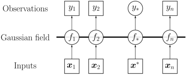
Schematic of a Gaussian process f. The values in squares are known while values in circles are unknown.
Given this structure, the GRP model is fully specified by choosing the kernel function and the optimal kernel hyperparameters. A pragmatic way to choose the kernel and hyperparameters is to separate the available data into test and training data sets and select the GPR model that performs best at predicting the test data given the training data. The model that performs best will have the lowest test error, where test error is a function of the known values y* and the predictions . Additional information on separating between test and training samples for AFM data is given in Appendix Appendix A. Ultimately, GPR will likely lead to a better approximation of cell properties between the measured data points than strategies such as linear interpolation, illustrated in Appendix Appendix B.
3. Results
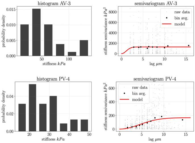
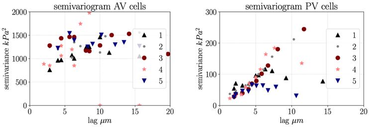
As introduced in Section 1, AFM is commonly used to make spatially distributed measurements of cell stiffness and cell height. Here, we re-visit an experimental analysis of AVICs and PVICs where it was previously shown using standard methods that the two cell types have different average mechanical properties (Merryman et al., 2007). From our analysis, we obtain novel insights into the characteristics of AVICs and PVICs. First, we report global Moran’s I and associated z-score zI, for measurements of scalar stiffness represented by apparent elastic modulus E for five aortic valve cells and six pulmonary valve cells (Table 1). None of the five AVICs showed statistically significant spatial correlation in stiffness (p < 0.001) at the length scale of sampling while six out of six PVICs showed statistically significant spatial autocorrelation. We then show a representative histogram and semivariogram for an AVIC with low spatial autocorrelation and a PVIC with high spatial autocorrelation (Fig. 4). Though the histograms look qualitatively similar, the semivariograms look qualitatively different. This is consistent with the empirical semivariogram plots for the other AVICs and PVICs (Fig. 5). Overall, AVICs show much higher variance for every lag distance, and the decrease in variance at small lag distances is much less pronounced than in the PVICs. Though the sample size is relatively small, the difference between the two cell types is consistent, both in the present study and in related studies.
Table 1:
Moran’s I and zI for Aortic Valve (AV) cells and Pulmonary Valve (PV) cells. The cells marked with ★ show statistically significant spatial autocorrelation with p < 0.001 at the length scale of sampling. We note that AV-2 shows statistically significant spatial autocorrelation with p < 0.05.
| cell no. | I | zi | cell no. | I | zi |
|---|---|---|---|---|---|
| AV-1 | 0.095 | 1.15 | ★ PV-1 | 0.42 | 6.33 |
| AV-2 | 0.27 | 2.39 | ★ PV-2 | 0.50 | 7.68 |
| AV-3 | −0.012 | 0.092 | ★ PV-3 | 0.57 | 9.25 |
| AV-4 | −0.082 | −0.31 | ★ PV-4 | 0.70 | 10.29 |
| AV-5 | 0.023 | 0.11 | ★ PV-5 | 0.39 | 6.24 |
Figure 4:
Upper left: histogram for an AVIC; Upper right: semivariogram for an AVIC where there is no statistically significant spatial correlation (Table 1); Lower left: histogram for a PVIC; Lower right: semivariogram for a PVIC where there is statistically significant spatial correlation (Table 1).
Figure 5:
Left: empirical semivariograms for five AVICs; right: empirical semivariograms for five PVICs. For the AVICs, low lag distance does not correspond to low semivariance. For the PVICs, low lag distance corresponds to low semivariance which indicates that values are spatially correlated.
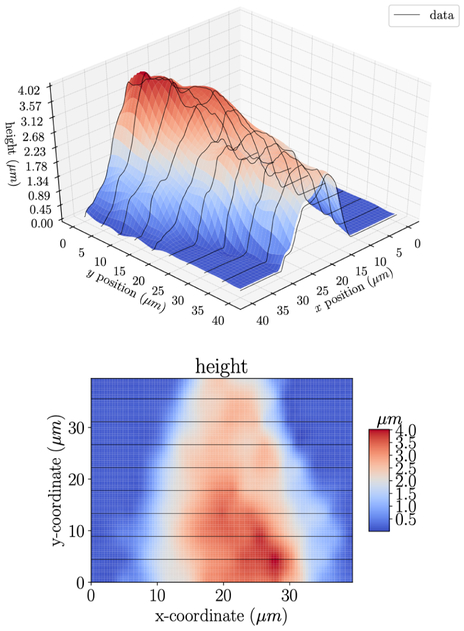
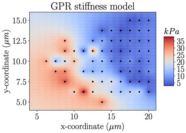
Next, we show the results of using Gaussian process regression to interpolate both height data and stiffness data. First, we show the interpolated heights for a single cell measured by AFM (Fig. 6). Mean absolute test error under 0.2 μm, reported in Appendix Appendix A, was a good approximation for the error with this method. In addition, we show the interpolated stiffness values for a single cell measured by AFM (Fig. 7). Using leave one out cross validation, where all but one data points are included in the model at a time, we can get an understanding of model error on unseen data. For the cell shown, PV-4, which had high spatial autocorrelation, the mean absolute error was under 3 kPa. Additional analysis of this error is given in Appendix Appendix B. For the cells which show no significant spatial correlation, i.e. the AVIC cells, GPR is not a good strategy to model spatial variations in stiffness because stiffness will not be well predicted by position.
Figure 6:
Gaussian process regression interpolation of height data from an AFM study on an aortic valve cell. The black lines indicate the raw experimental data while the surface is the GPR model. Note that the z axis is magnified.
Figure 7:
Gaussian process regression interpolation of stiffness data from an AFM study on a pulmonary valve cell. The black markers indicate the locations where experimental data is available. Based on further analysis given in Appendix Appendix B, the mean absolute error of this method on unseen data (in this case held out test data) is under 3 kPa.
4. Discussion
4.1. Major findings
The methods described in this paper are simple yet powerful tools to interpret and model spatial heterogeneity in AFM data. With the simple methods described in Section 2, we are able to both quantify experimentally observed spatial autocorrelation and introduce a strategy towards better capturing spatially varying data. When we compute Moran’s I for stiffness measurements in multiple AVICs and PVICs, following the method in Section 2.2, we are able to show that there are differences in spatial autocorrelation between the two cell types. Creating empirical semivariograms, following the method in Section 2.3, further exposes the fundamental distinction between the two cell types and illustrate the distance over which PVIC stiffness is correlated.
For the experimental measurements that display spatial autocorrelation, Gaussian process regression is a suitable method for interpolating data points. As emphasized in Section 2.4, care must be taken when considering the separation of test and training data. The pragmatic approach put forward here for dealing with the directionally dependent spacing of AFM height data is appealing because of its simplicity. Furthermore, we show an example of GPR being used to interpolate cell stiffness in PVICs. We anticipate that GPR and similar enhanced interpolation strategies will be key to creating realistic computational cell models that account for spatial heterogeneity in cell geometry and properties. When cell properties are not spatially correlated, alternative methods must be introduced to create representative cell models (Ostoja-Starzewski, 2006).
The present findings reinforce and extend previous results that show differences in the mean cell stiffness, αSMA levels, stress fiber stiffness, and extracellular matrix remodeling capabilities between aortic and pulmonary VICs Merryman et al. (2006, 2007); Sakamoto et al. (2016, 2017). In particular, previous studies have found via micropipette aspiration and AFM indentation that PVICs are less stiff than AVICs, AVICs express higher αSMA levels, intrinsically stronger stress fibers, and will typically remodel collagen gels at an accelerated rate. In this work, it was observed that PVICs exhibit much higher levels of spatial correlation in stiffness than their AVIC counterparts (Fig. 5). Essentially, AVICs have a more heterogeneous stiffness. This indicates that some sub-cellular stress-fiber formation activity is likely quite different between the two cell types. One possible explanation for this is that the stress fiber architecture of AVIC form more focal adhesion compared to the “smoother” spatial features of the PVICs. The underlying mechanism driving this difference could be connected to highly localized stress fiber formation in AVICs. We also note that another mechanisms driving this difference may be that AVICs and PVICs responds differently to cell culture conditions due to different degrees of deviation from their native chemical and mechanical environment. Future research will be needed to clarify these insights and compare the behavior of these isolated cells to cells in the native tissue.
4.2. Broader findings
Putting this in a broader perspective, distinguishing between cells types and detecting changes in cell state and behavior is critical for understanding tissue and organ scale function (Ayoub et al., 2017; Rego et al., 2018). Given that VICs are present in all heart valves, yet likely subject to dramatically different valve-specific mechanical loading conditions throughout their lifetime (Ayoub et al., 2018), quantitative methods for determining the difference between cell types are quite meaningful. With this enhanced strategy for quantifying experimental data, it is possible to both detect these differences and more robustly consider their implications in the broader context of multiscale modeling (Lee et al., 2017; Lejeune and Linder, 2018; Lejeune et al., 2019). Furthermore, this clear demonstration of spatial heterogeneity within individual cells shows that experiments with techniques such as micropipette aspiration may be missing critical information about the heterogeneous distribution of mechanical properties within the cell (Sakamoto et al., 2016).
Looking forward, capturing and modeling the spatial variation in cell properties is an important step towards understanding both cell mechanics and cell-substrate/ cell-matrix interaction. Fundamentally, this methodology will lead to a better understanding of how sub-cellular components come together and contribute to the mechanical behavior of the whole cell. And, it will contribute to our understanding of how spatially heterogeneous cell behavior ultimately influences tissue function. In addition, information on spatial heterogeneity of cell stiffness will lead to enhanced computational models for calculating the forces that cells experience that, unlike many approaches, will not assume cell stiffness is homogeneous. Computational models will be particularly useful for comparing isolated cells to cells in the native tissue environment. Furthermore, additional understanding of the inherent heterogeneity in biological samples will interface well with methods for rapidly acquiring AFM measurements (Hartman and Andersson, 2017; Huang and Andersson, 2012).
4.3. Conclusions
In conclusion, applying tools from spatial statistics to AFM data will provide substantial new insight and lead to a deeper understanding of the properties of biological cells. We were able to demonstrate that pulmonary valve interstitial cells display higher levels of spatial autocorrelation of stiffness than aortic valve interstitial cells. Thus, the addition of spatial statistics can contribute to our fundamental understanding of the differences between these cell types. The methods presented in this paper are also only a small subset of what is available in the spatial statistics literature. For example, Geary’s C and Getis-Ord Gi* are other single variable measurements of spatial autocorrelation (Geary, 1954; Getis and Ord, 1992), and AFM indentation may be used to approximate indentation parameters beyond apparent elastic modulus (Putman et al., 1994). Furthermore, there are extensions of these techniques to understand correlations in both space and time (Sherman, 2011). Biomechanics researchers working with spatially heterogeneous AFM data should consider these approaches in their analysis.
Acknowledgements
This work was funded by the Peter O’Donnell, Jr. Postdoctoral Fellowship at the Institute for Computational Engineering and Sciences at The University of Texas at Austin to EL and NIH grants HL073021, HL142504, and HL119297 to MSS.
Appendix
Appendix A. Separating test and training data for Gaussian Process Regression
A pragmatic strategy for constructing a GPR model is to separate data into a test set and a training set and evaluate model performance as the error on the test set. Much of this workflow is accomplished by a package such as sklearn-learn (Pedregosa et al., 2011). Here we note that it is important to consider what a meaningful split of test and training data is given the nature of the available data. More specifically, consider the AFM height measurements where the scanning probe is moved in a line along the sample surface (Fig. 1). As the tip passes over the cell, multiple data points are recorded with a fixed y-value so the data is quite dense in the x-direction. The tip then passes over another line with a fixed y-value such that the distance between data points is much greater in the y-direction than in the x. If we first consider the AFM height data in one y plane, where the data available is quite dense and uniformly spaced, separating test and training data is straightforward. To demonstrate this, we show the decrease in mean absolute test error as the number of training samples is increased and the resulting closer match between the predicted height of the GPR model and the measured height (Fig. A.8).
Figure A.8:
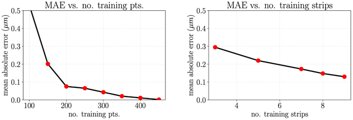
Left: the mean absolute error (MAE) of the test predictions decreases as the number of training points increases; Center: GPR model fit with five sample points compared to raw data; Right: GPR model fit with 50 sample points compared to raw data.
Next, we consider the AFM height data in both the x and y planes. If we separate the test and training data without considering that the data is unevenly spaced, the reported test error is artificially low and the GPR parameters may be tuned such that the model is overfitting (Fig. A.9 left). Instead, to get a more realistic impression of test error and to select the GPR model parameters that will best predict unseen data, we must separate test and training error by grouping entire “strips” of data with identical y-coordinates corresponding to one pass of the AFM tip probe. When we do this, we see that the test error decreases with each additional “strip” of data and is notably higher than with the previous uninformed test and training data separation method (Fig. A.9 right). Furthermore, the best performing kernel may be different than the case where no special consideration is given to the separation of test and training data. The resulting GPR model can then be used to interpolate height data in the regions between each pass of the AFM tip (Fig. 6 right). When the data is evenly spaced in both dimensions, as is the case with the AFM stiffness data available, this additional consideration is not necessary.
Figure A.9:
Left: MAE of the test predictions approaches zero as the number of naively selected training points increases; Right: MAE of the test prediction decreases as the number of strips of training points increases.
Appendix B. Comparing Gaussian Process Regression to linear interpolation
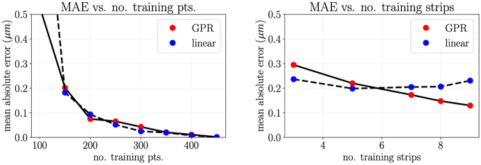
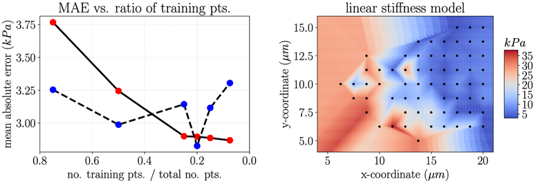
When the AFM data is quite densely spaced, for example in the x-direction of height measurements, the strategy for inferring values between measured data points is less important. However, when the spacing between data points is larger, for example in the y-direction of height measurements and the grid of stiffness measurements, critically evaluating how to infer these values matters. To illustrate this, we compare the mean absolute error (MAE) in height prediction computed with GPR and linear interpolation with respect to the number of training points (Fig. B.10 left) and the number of training strips (Fig. B.10 right). Though there is no apparent difference between the two methods for the incorrect test and training data separation, discussed in Appendix Appendix A, there is a notable difference for the correct test and training data separation. Interpolation with GPR results in a lower MAE, and the MAE for GPR appears to decrease with respect to the addition of more training data in a way that the linear interpolation strategy does not. Similar behavior is observed for interpolating stiffness, where MAE reliably decreases with the addition of more training data for GPR but not for linear interpolation (Fig. B.11 left). Of course, there are many other potential strategies besides GPR and linear interpolation (Friedman et al., 2001). For future endeavors in computational modeling of cells based on AFM data, we recommend critically evaluating multiple data-specific strategies for interpolating between measured data points. Noting the difference between GPR (Fig. 7) and linear interpolation (Fig. B.11 right) emphasizes this point.
Figure B.10:
Left: Comparison between MAE of the test predictions for GPR and linear interpolation as the number of naively selected training points increases; Right: Comparison between MAE of the test predictions for GPR and linear interpolation as the number of strips of training points increases.
Figure B.11:
Left: Comparison between MAE of the test predictions for GPR and linear interpolation as the fraction of data included in the training set increase; Right: Plot of linear interpolation of stiffness (the nearest interpolated point is used to fill in the extrapolated regions).
Footnotes
Conflict of interest
The authors declared that there are no conflicts of interest.
Publisher's Disclaimer: This is a PDF file of an unedited manuscript that has been accepted for publication. As a service to our customers we are providing this early version of the manuscript. The manuscript will undergo copyediting, typesetting, and review of the resulting proof before it is published in its final citable form. Please note that during the production process errors may be discovered which could affect the content, and all legal disclaimers that apply to the journal pertain.
References
- Ayoub S, Ferrari G, Gorman RC, Gorman JH III, Schoen FJ, Sacks MS, 2011. Heart valve biomechanics and underlying mechanobiology. Comprehensive Physiology 6, 1743–1780. [DOI] [PMC free article] [PubMed] [Google Scholar]
- Ayoub S, Lee CH, Driesbaugh KH, Anselmo W, Hughes CT, Ferrari G, Gorman RC, Gorman JH, Sacks MS, 2017. Regulation of valve interstitial cell homeostasis by mechanical deformation: implications for heart valve disease and surgical repair. Journal of The Royal Society Interface 14, 20170580. [DOI] [PMC free article] [PubMed] [Google Scholar]
- Ayoub S, Tsai KC, Khalighi AH, Sacks MS, 2018. The three-dimensional microenvironment of the mitral valve: insights into the effects of physiological loads. Cellular and Molecular Bioengineering 11, 291–306. [DOI] [PMC free article] [PubMed] [Google Scholar]
- Cressie NAC, 1993. Statistics for Spatial Data. Wiley. [Google Scholar]
- Cross SE, Jin YS, Tondre J, Wong R, Rao J, Gimzewski JK, 2008. Afm-based analysis of human metastatic cancer cells. Nanotechnology 19, 384003. [DOI] [PubMed] [Google Scholar]
- Diblasi A, Bowman A, 2001. On the use of the variogram in checking for independence in spatial data. Biometrics 57, 211–218. [DOI] [PubMed] [Google Scholar]
- Friedman J, Hastie T, Tibshirani R, 2001. The elements of statistical learning. volume 1 Springer series in statistics New York. [Google Scholar]
- Gavara N, 2017. A beginner’s guide to atomic force microscopy probing for cell mechanics. Microscopy research and technique 80, 75–84. [DOI] [PMC free article] [PubMed] [Google Scholar]
- Geary RC, 1954. The contiguity ratio and statistical mapping. The incorporated statistician 5, 115–146. [Google Scholar]
- Getis A, Ord JK, 1992. The analysis of spatial association by use of distance statistics. Geographical analysis 24, 189–206. [Google Scholar]
- Goodchild MF, 1986. Spatial autocorrelation. volume 47 Geo Books. [Google Scholar]
- Haase K, Pelling AE, 2015. Investigating cell mechanics with atomic force microscopy. Journal of The Royal Society Interface 12, 20140970. [DOI] [PMC free article] [PubMed] [Google Scholar]
- Hartman B, Andersson SB, 2017. Feature tracking for high speed afm: Experimental demonstration, in: 2017 American Control Conference (ACC), IEEE; pp. 773–778. [Google Scholar]
- Huang P, Andersson SB, 2012. Fast scanning in afm using non-raster sampling and time-optimal trajectories, in: 2012 IEEE 51st IEEE Conference on Decision and Control (CDC), IEEE; pp. 5073–5078. [Google Scholar]
- Lee CH, Zhang W, Feaver K, Gorman RC, Gorman JH, Sacks MS, 2017. On the in vivo function of the mitral heart valve leaflet: insights into tissue-interstitial cell biomechanical coupling. Biomechanics and modeling in mechanobiology 16, 1613–1632. [DOI] [PMC free article] [PubMed] [Google Scholar]
- Lejeune E, Dortdivanlioglu B, Kuhl E, Linder C, 2019. Understanding the mechanical link between oriented cell division and cerebellar morphogenesis. Soft matter. [DOI] [PubMed] [Google Scholar]
- Lejeune E, Linder C, 2017. Quantifying the relationship between cell division angle and morphogenesis through computational modeling. Journal of theoretical biology 418, 1–7. [DOI] [PubMed] [Google Scholar]
- Lejeune E, Linder C, 2018. Understanding the relationship between cell death and tissue shrinkage via a stochastic agent-based model. Journal of Biomechanics 73, 9–17. [DOI] [PubMed] [Google Scholar]
- Luo Q, Kuang D, Zhang B, Song G, 2016. Cell stiffness determined by atomic force microscopy and its correlation with cell motility. Biochimica et Biophysica Acta (BBA)-General Subjects 1860, 1953–1960. [DOI] [PubMed] [Google Scholar]
- Mälicke M, Schneider HD, 2018. mmaelicke/scikit-gstat: Geostatistical variogram toolbox (version v0.2.2). [Google Scholar]
- Matheron G, 1963. Principles of geostatistics. Economic geology 58, 1246–1266. [Google Scholar]
- Mathur AB, Collinsworth AM, Reichert WM, Kraus WE, Truskey GA, 2001. Endothelial, cardiac muscle and skeletal muscle exhibit different viscous and elastic properties as determined by atomic force microscopy. Journal of biomechanics 34, 1545–1553. [DOI] [PubMed] [Google Scholar]
- Merryman WD, Liao J, Parekh A, Candiello JE, Lin H, Sacks MS, 2007. Differences in tissue-remodeling potential of aortic and pulmonary heart valve interstitial cells. Tissue engineering 13, 2281–2289. [DOI] [PubMed] [Google Scholar]
- Merryman WD, Youn I, Lukoff HD, Krueger PM, Guilak F, Hopkins RA, Sacks MS, 2006. Correlation between heart valve interstitial cell stiffness and transvalvular pressure: implications for collagen biosynthesis. American Journal of Physiology-Heart and Circulatory Physiology 290, H224–H231. [DOI] [PubMed] [Google Scholar]
- Mitchel A, 2005. The ESRI Guide to GIS analysis, Volume 2: Spartial measurements and statistics. ESRI Guide to GIS analysis. [Google Scholar]
- Moran PA, 1950. Notes on continuous stochastic phenomena. Biometrika 37, 17–23. [PubMed] [Google Scholar]
- Nguyen N, Shao Y, Wineman A, Fu J, Waas A, 2016. Atomic force microscopy indentation and inverse analysis for non-linear viscoelastic identification of breast cancer cells. Mathematical biosciences 277, 77–88. [DOI] [PubMed] [Google Scholar]
- Ostoja-Starzewski M, 2006. Material spatial randomness: From statistical to representative volume element. Probabilistic engineering mechanics 21, 112–132. [Google Scholar]
- Pedregosa F, Varoquaux G, Gramfort A, Michel V, Thirion B, Grisel O, Blondel M, Prettenhofer P, Weiss R, Dubourg V, Vanderplas J, Passos A, Cournapeau D, Brucher M, Perrot M, Duchesnay E, 2011. Scikit-learn: Machine learning in Python. Journal of Machine Learning Research 12, 2825–2830. [Google Scholar]
- Putman C, Van der Werf KO, de Grooth BG, van Hulst NF, Greve J, 1994. Viscoelasticity of living cells allows high resolution imaging by tapping mode atomic force microscopy. Biophysical journal 67, 1749–1753. [DOI] [PMC free article] [PubMed] [Google Scholar]
- Radmacher M, Tillamnn R, Fritz M, Gaub H, 1992. From molecules to cells: imaging soft samples with the atomic force microscope. Science 257, 1900–1905. [DOI] [PubMed] [Google Scholar]
- Rasmussen CE, Williams CK, 2006. Gaussian processes for machine learning. The MIT Press. [Google Scholar]
- Rego BV, Khalighi AH, Drach A, Lai EK, Pouch AM, Gorman RC, Gorman JH III, Sacks MS, 2018. A noninvasive method for the determination of in vivo mitral valve leaflet strains. International journal for numerical methods in biomedical engineering 34, e3142. [DOI] [PubMed] [Google Scholar]
- Rego BV, Sacks MS, 2017. A functionally graded material model for the transmural stress distribution of the aortic valve leaflet. Journal of biomechanics 54, 88–95. [DOI] [PMC free article] [PubMed] [Google Scholar]
- Rigato A, Rico F, Eghiaian F, Piel M, Scheuring S, 2015. Atomic force microscopy mechanical mapping of micropatterned cells shows adhesion geometry-dependent mechanical response on local and global scales. ACS nano 9, 5846–5856. [DOI] [PMC free article] [PubMed] [Google Scholar]
- Ripley BD, 2005. Spatial statistics. volume 575 John Wiley & Sons. [Google Scholar]
- Sacks MS, Khalighi A, Rego B, Ayoub S, Drach A, 2017. On the need for multi-scale geometric modelling of the mitral heart valve. [DOI] [PMC free article] [PubMed] [Google Scholar]
- Sakamoto Y, Buchanan RM, Sacks MS, 2016. On intrinsic stress fiber contractile forces in semilunar heart valve interstitial cells using a continuum mixture model. Journal of the mechanical behavior of biomedical materials 54, 244–258. [DOI] [PMC free article] [PubMed] [Google Scholar]
- Sakamoto Y, Buchanan RM, Sanchez-Adams J, Guilak F, Sacks MS, 2017. On the functional role of valve interstitial cell stress fibers: a continuum modeling approach. Journal of biomechanical engineering 139, 021007. [DOI] [PMC free article] [PubMed] [Google Scholar]
- Sherman M, 2011. Spatial statistics and spatio-temporal data: covariance functions and directional properties. John Wiley & Sons. [Google Scholar]
- Stein ML, 1999. Statistical Interpolation of Spatial Data: Some Theory for Kriging. Springer. [Google Scholar]
- Steiniger S, Hunter AJ, 2012. Free and open source gis software for building a spatial data infrastructure. Geospatial free and open source software in the 21st century, 247–261. [Google Scholar]
- Yeow N, Tabor RF, Garnier G, 2017. Atomic force microscopy: From red blood cells to immunohaematology. Advances in colloid and interface science 249, 149–162. [DOI] [PubMed] [Google Scholar]


