Abstract
Circular RNAs (circRNAs), with their crucial roles in gene regulation and disease development, have become rising stars in the RNA world. To understand the regulatory function of circRNAs, many studies focus on the interactions between circRNAs and RNA-binding proteins (RBPs). Recently, the abundant CLIP-seq experimental data has enabled the large-scale identification and analysis of circRNA–RBP interactions, whereas, as far as we know, no computational tool based on machine learning has been proposed yet. We develop CRIP (CircRNAs Interact with Proteins) for the prediction of RBP-binding sites on circRNAs using RNA sequences alone. CRIP consists of a stacked codon-based encoding scheme and a hybrid deep learning architecture, in which a convolutional neural network (CNN) learns high-level abstract features and a recurrent neural network (RNN) learns long dependency in the sequences. We construct 37 data sets including sequence fragments of binding sites on circRNAs, and each set corresponds to an RBP. The experimental results show that the new encoding scheme is superior to the existing feature representation methods for RNA sequences, and the hybrid network outperforms conventional classifiers by a large margin, where both the CNN and RNN components contribute to the performance improvement.
Keywords: circular RNA, RNA–protein interaction, deep learning, codon-based encoding
INTRODUCTION
Circular RNAs (circRNAs) are a special type of noncoding RNAs, whose structures are characterized by nonlinear back-splicing. Although circRNAs are categorized as noncoding RNAs, their potential to code for proteins has been reported recently (Pamudurti et al. 2017). Compared to linear RNA molecules, circRNAs are more stable and conserved across species (Jeck et al. 2013). Natural circRNAs were discovered 20 years ago, whereas their important roles in gene regulation and disease development have attracted public attention only in recent years (Hansen et al. 2013a; Li et al. 2015).
Benefiting from the high-throughput sequencing techniques, a large number of circRNA loci have been discovered in human genomes. Various databases and computational methods have been developed for circRNAs. For instance, circBase provides visualization tools for browsing a large number of circRNAs at the genome scale and identifying circRNAs in sequencing data (Glažar et al. 2014). CIRCpedia also allows users to search, browse, and download circRNAs with expression profiles in various cell types/tissues including disease samples (Wang et al. 2017). CircR2Disease focuses on the associations between circRNAs and diseases (Fan et al. 2018), and CircInteractome houses the RBP/miRNA-binding sites on human circRNAs (Dudekula et al. 2016).
According to previous studies, circRNAs play their regulatory functions via sponging microRNAs (miRNAs) (Hansen et al. 2013a,b; Memczak et al. 2013) and RNA-binding proteins (RBPs) (Du et al. 2016; Xia et al. 2016). To detect the interactions between proteins and RNAs, high-throughput techniques have been developed, including both in vivo and in vitro experiments (Ray et al. 2013; Van Nostrand et al. 2016). Based on the high-throughput data, a lot of computational tools have been developed. For instance, Li et al. (2017b) applied a soft-clustering method, RBPgroup, to various CLIP-seq data sets, and grouped RBPs that specifically bind to the same RNAs. Li et al. (2017a) reported an approach circScan to identify regulatory interactions between circRNAs and RBPs by discovering back-splicing reads from cross-linking and immunoprecipitation followed by CLIP-seq data. In recent years, the identification of protein–RNA interactions based on machine learning methods has been a hot topic in the bioinformatics field (Li et al. 2013). The existing methods fall into two categories, predicting the binding sites in the protein chains and RNA chains, respectively. The prediction in the RNA chains is more difficult because of the limited information source (mainly the RNA sequences), whereas for proteins, functional annotation knowledge or signal peptide could be utilized (Zhang et al. 2010; Yan et al. 2016).
The prediction of protein–RNA-binding sites is essentially a classification problem, involving both feature representations for sequences and classification models. Traditionally, RNA sequence classification adopts handcrafted features, which are mainly extracted from statistical properties. For instance, k-tuple nucleotide composition (Zhang et al. 2011) is the most basic method, which lays the foundation for a series of statistical feature extraction methods of RNAs. Note that RNAs have four different nucleotides, “A (adenine),” “G (guanine),” “C (cytosine),” and “U (uracil)”; thus, k-tuples have 4k different combinations, which means that each RNA sequence corresponds to a 4k-dimensional feature vector. This type of feature can capture the short-range or local sequence order information (Chen et al. 2014).
In the past decade, with the rise of deep learning, sequence encoding methods have attracted more and more attention. One-hot encoding is a simple and common feature representation method, which has been widely used in biological sequence classification (Baldi et al. 2002). For RNA/DNA sequences, each nucleotide is encoded as a four-dimensional binary vector, which can work with both traditional classifiers and deep learning models. Furthermore, researchers have incorporated the secondary structure of RNAs into the one-hot encoding method (Park et al. 2017).
In addition to the feature representation, various machine learning methods have been proposed in the prediction of molecular interactions. For instance, support vector machines (SVMs) and random forests (RFs) have been applied to protein–protein prediction (Shen et al. 2007) and RNA–protein prediction (Muppirala et al. 2011). Deep learning models have also emerged—for example, DeepBind based on convolutional neural networks (CNNs) (Alipanahi et al. 2015), iDeep based on fusing multiple features (Pan and Shen 2017), and iDeepE based on local and global CNNs (Pan and Shen 2018).
Despite the progress on predicting interactions between linear RNAs and RBPs, to the best of our knowledge, computational tools for identifying the interactions between circRNAs and RBPs have not been reported yet. Although the existing methods for linear RNAs could be applied, customized tools for circRNAs are needed for the following reasons. First, the mechanisms of circRNAs interacting with RBPs are different from those of other types of RNAs, thus the existing methods may not generalize well to circRNAs. Second, circRNAs have limited information for the prediction. For linear RNAs, besides the sequences, secondary structures information is usually extracted and incorporated into the predictor. Compared to linear RNAs, which have free ends and diversified secondary structure elements, circRNAs are more topologically constrained (a covalently closed continuous loop). Third, there is still room to improve the current predictors for RNA–protein interactions: (i) The conventional one-hot representation may lose much information of sequence patterns because of the low dimensionality and simple encoding scheme; and (ii) the capabilities of deep learning models have not been fully exploited.
In this study, we propose a deep learning–based model for predicting RBP-binding sites on circRNAs using sequences alone, named CRIP. The contributions include:
Construct benchmark data sets of circRNA segments binding to RBPs, and propose the specific predictor for the identification of RBP-binding sites on circRNAs.
Design a new encoding scheme to represent RNA sequences, and apply it to the prediction of RBP-binding sites on both circRNAs and linear RNAs.
Use a hybrid deep neural network to further improve the prediction performance.
RESULTS
As the information source for predicting circRNA–RBP interactions is limited, the feature extraction from circRNA sequences is crucial to the prediction system. Instead of using the traditional one-hot encoding method, we propose a stacked codon-based encoding method to get an initial representation for the RNA sequences. Then we adopt a CNN to learn high-level features from the initial representation and a long short-term memory (LSTM) network to capture the long dependency within the sequences. The outputs of all the time steps are concatenated and fed into two fully connected layers to yield the final output probability. The whole pipeline is shown in Figure 1.
FIGURE 1.
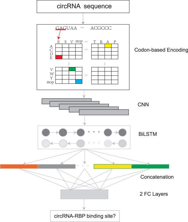
Flowchart of CRIP. CRIP represents RNA sequences by stacked codon-based encoding method. The encoded vectors are fed into a CNN module followed by a BiLSTM module and further classified via two fully connected layers.
In the following sections, we first investigate the contributions of feature encoding and deep learning models, respectively. Then, we compare CRIP with the existing methods for predicting RNA–protein interactions. Last, we discuss the performance difference between the predictions of linear RNAs and circRNAs.
Both the new feature encoding scheme and hybrid DNN contribute to the performance improvement
Investigation on feature encoding
The methods for representing RNA sequences fall into two categories (i.e., feature engineering and sequence encoding), which work with traditional machine learning methods and deep learning methods, respectively. For instance, in Shen et al. (2007) and Muppirala et al. (2011), k-mer frequencies were used as features and classified by SVMs and RFs, whereas some recent methods—for example, DeepBind (Alipanahi et al. 2015), iDeep (Pan and Shen 2017), and iDeepS (Pan et al. 2018)—adopted one-hot encoding and deep learning models as classifiers.
With the increasing applications of deep learning in sequence analysis, traditional feature extraction methods have been largely replaced by sequence encoding methods. However, the classic one-hot encoding has obvious drawbacks. For RNA/DNA sequences, each nucleotide is encoded as a four-dimensional binary vector. Such a low-dimensional feature representation may be incompetent to characterize the sequence information well; in particular, the sequence context information is not encoded in the one-hot encoding method.
To incorporate context information and get an expanded vector space retaining more sequence features, we propose a new method, called stacked codon–based encoding.
Inspired by the coding potential of circRNAs (Pamudurti et al. 2017), we map each group of three consecutive nucleotides (i.e., 3-mer) in the circRNA sequences into a pseudo–amino acid. The mapping is similar to the translation of codons, except that the mapping is conducted in an overlapping manner because of the indeterminacy of the starting site. Also, because this is not a real translation process, we allow stop codons in the middle of sequences. As we extract 3-mers from RNA sequences using a sliding window with step size 1, the stacked codon–based encoding method can be regarded as a variant of the k-mer method (k = 3). Because there are 64 combinations of 3-mers and only 21 different symbols (20 amino acids plus a stop codon), each amino acid may correspond to multiple codons. This method not only reduces the feature dimensionality of a classic k-mer method but also groups the 3-mers with common biological properties. Finally, we encode the “amino acid” sequences by the conventional one-hot method—that is, each symbol is converted into a 21-D binary vector, where only one element is nonzero. (The new method is formularized in Materials and Methods.)
To demonstrate the advantage of the stacked codon encoding method, we consider another encoding scheme, called IUPAC (Cornishbowden 1985), which provides another alphabet consisting of 16 characters. IUPAC considers the genetic variation; thus, each symbol in its alphabet corresponds to a polymorphic status of nucleic acids, like “A or C” and “not G”, as shown in Supplemental Table S1 (Johnson 2010). In this paper, the IUPAC method refers to the extended one-hot encoding using the IUPAC alphabet.
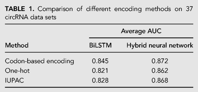
We compare the average AUCs of classic one-hot, IUPAC encoding, and the stacked codon-based encoding in Table 1. These encoding methods work with two different classifiers, namely, BiLSTM (i.e., the RNN part in the hybrid neural network) and the hybrid neural network, respectively. In both cases, our method achieves the best performance, and IUPAC outperforms one-hot slightly. Obviously, our method and IUPAC have larger alphabets than the conventional one-hot encoding, and the extended encoding space is helpful to retain sequence features. As can be seen, benefiting from the CNN module, all the three encoding methods get improved accuracy, and the performance gap becomes smaller compared to using only the LSTM component, suggesting that the deep learning architecture can compensate for the initial simple features.
TABLE 1.
Comparison of different encoding methods on 37 circRNA data sets
Investigation on learning models
As our model includes a CNN module and a BiLSTM module, to evaluate the contribution of each module in the hybrid neural network, we examine the performance of individual modules. The results are shown in Figure 2.
FIGURE 2.
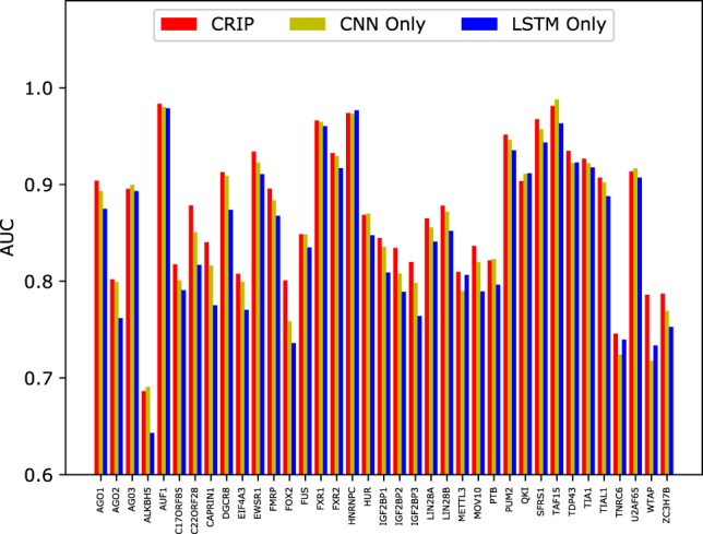
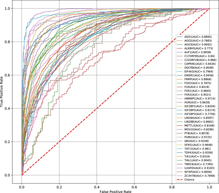
The AUCs of the LSTM module, CNN module, and the hybrid model on 37 circRNA data sets.
Apparently, the single modules do not perform as well as the hybrid model, which has an average AUC of 0.872. The ROC curves of CRIP on 37 data sets are shown in Figure 3. The CNN module is better than the BiLSTM module (0.861 vs. 0.845). The results suggest that CNN can extract more accurate sequence information for the detection of RNA–protein interactions.
FIGURE 3.
The ROC curves obtained by CRIP for 37 circRNA data sets.
CRIP outperforms the existing predictors designed for linear RNAs
Comparison with traditional machine learning methods
Regardless of structure, the identification of RBP-binding sites for any types of RNAs relies on the same information source (i.e., RNA sequences). Thus, we apply previous methods designed for linear RNAs to circRNAs. In Muppirala et al. (2011), the authors proposed RPISeq-SVM and RPISeq-RF to identify RNA–protein interactions, which used two classic shallow learning models, SVMs and RFs. And the RNA sequence features were represented by normalized 4-mer composition. Here we implement these two methods, which are trained and evaluated using the same 37 circRNA data sets as CRIP. The results are shown in Figure 4.
FIGURE 4.
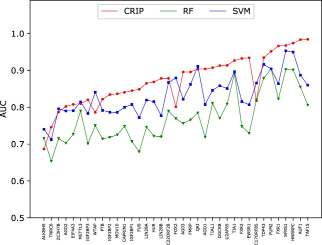
Comparison of AUCs between CRIP and the predictors based on traditional machine learning models on 37 circRNA data sets.
The advantages of CRIP over the traditional learning methods are obvious. Of the 37 data sets, CRIP achieves the best results on 30 data sets. The average AUC of CRIP is 0.872, which is 4.6% higher than that of the SVM (0.834), and 13.4% higher than that of RF (0.769), demonstrating the advantages of the proposed deep model over traditional learning methods.
Comparison with the existing deep learning methods
To further assess the performance of CRIP, we compare it with the deep learning–based predictors, including DeepBind (Alipanahi et al. 2015) and iDeepS (Pan and Shen 2018). Here iDeep is excluded in the comparison because it requires annotation information of gene regions and clip-cobinding (Pan and Shen 2017). DeepBind utilizes only sequence features and adopts a sequence CNN, whereas iDeepS integrates both sequence and secondary structure information and adopts a similar model architecture as CRIP. Because these two methods were designed for linear RNAs rather than circRNA, to perform a fair comparison, we conduct the experiments on the benchmark sets of linear RNAs, including 31 data sets (Pan and Shen 2017).
As shown in Figure 5, CRIP achieves the best results for most of the RBPs. For some RBPs, like the Argonaute family of proteins (AGO), CRIP performs much better than the two other methods. iDeepS has a slight advantage over DeepBind because the secondary structure information incorporated in iDeepS improves the prediction accuracy. On average, CRIP obtains an AUC value of 0.856, which is higher than that of DeepBind (0.835) and iDeepS (0.839). The results demonstrate that CRIP not only applies to linear RNAs, but also improves the average AUC by ∼0.02 compared with the state-of-the-art deep models designed for linear RNAs.
FIGURE 5.
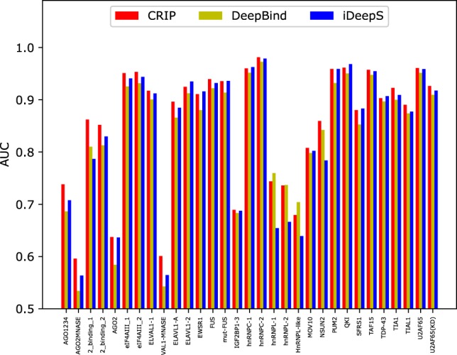
Performance comparison of the AUCs of DeepBind, iDeepS, and CRIP on 31 linear RNA data sets.
The models trained on linear RNAs could not simply be applied to circRNAs
Previous studies have used both shallow and deep learning models for predicting RNA–protein interactions, but none of them was designed for circRNAs. Note that there are some RBPs shared by circRNAs and other types of RNAs, thus we compare the RBPs used in this study and in previous studies (Pan and Shen 2018; Pan et al. 2018). There are 11 RBPs common to linear RNAs and circRNAs; we first check whether the predictors trained on linear RNAs can be generalized to circRNAs.
For each circRNA test set of the 11 shared RBPs, we compare the performance of CRIP with iDeep*.6 Figure 6 shows the prediction results of iDeep* and CRIP for the 11 common RBPs. As can be seen, CRIP outperforms iDeep* on all of the 11 data sets. Especially for FUS, HNRNPC, and MOV10, CRIP improves the AUC by >10%, indicating that the training sequences in iDeep* (linear RNAs) may be very different from the test sequences (circRNAs), and that these two types of RNAs may differ in the interaction mechanisms with the same RBPs. The results demonstrate the necessity of developing a specific predictor for identifying binding sites on circRNA sequences, not only for new RBPs but also for the shared RBPs with linear RNAs.
FIGURE 6.
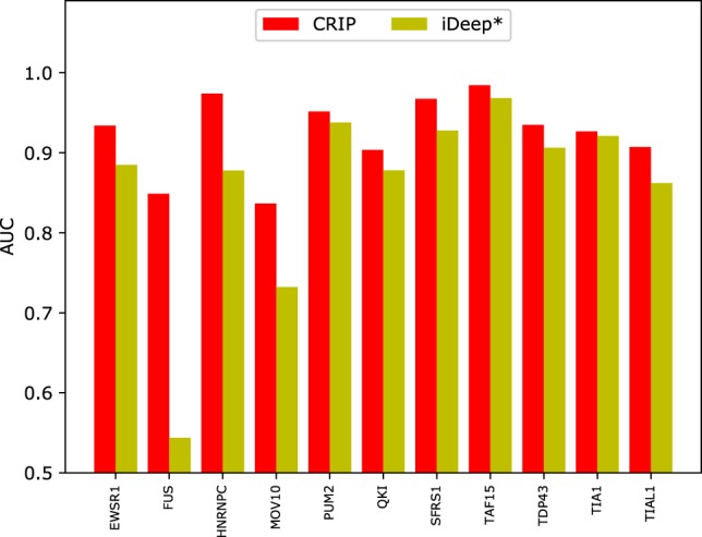
Comparison of AUCs of CRIP and iDeep* on the common RBPs. iDeep* is trained on linear RNAs and evaluated on the circRNA test set. CRIP is both trained and tested on circRNAs.
Linear RNAs and circRNAs binding to the same RBPs differ in their prediction accuracy
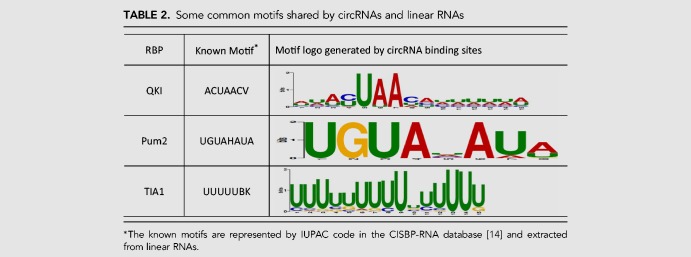
Compared with linear RNAs, circRNAs have their distinct structure and mechanism for binding to proteins, which motivates us to develop a new tool for identifying circRNA–protein interactions. As mentioned earlier in the subsection “CRIP outperforms the existing predictors designed for linear RNAs,” the proposed method is also applicable to any type of RNA, and circRNAs share some RBPs with linear RNAs. Thus, we compare the prediction performance of CRIP on the common RBPs for linear RNAs and circRNAs, as shown in Figure 7. As can be seen, the AUC values of linear RNAs and circRNAs differ a lot for some RBPs (e.g., FUS and SFRS1), and the AUCs for circRNAs are generally lower (on eight of 11 RBPs). The reasons for the performance difference are manifold. As a machine learning–based method, the performance of CRIP heavily relies on the scale of training data. In the linear RNA data sets, the number of training samples is fixed to be 5000 for each RBP. In contrast, when we construct the circRNA data set, we extract fragments from all binding sites, and the data sets vary in scale. Thus, if there are a lot of circRNA-binding sites for an RBP, the corresponding data set will have abundant training samples. Generally, a large training set will lead to good performance. For instance, the FUS and HNRNPC data sets of circRNA-binding sites are the two biggest, with 20,000 and 14,224 positive samples, respectively. CRIP achieves much better prediction performance on circRNAs than on linear RNAs for these two RBPs (the AUCs for the FUS data set are 0.930 and 0.849 for circRNAs and linear RNAs, respectively). However, there are a few exceptions. For the QKI data set, CRIP also performs better on circRNAs than on linear RNAs (0.960 vs. 0.904), whereas the number of positive training samples is only 1033, indicating that other factors also affect the prediction performance. Through a motif search using the MEME suite, we identify a conserved and concentrated pattern, “ACUAAC,” on the circRNAs binding to QKI. This motif has been verified and was included in the CISBP-RNA database (Ray et al. 2013). Similarly, we also find two other conserved patterns that are consistent with the motifs in CISBP-RNA: namely, “UGUA” for the binding to Pum2 and “UUUU” for the binding to TIA1 (Table 2). These two data sets have only 2829 and 2202 positive samples, respectively, whereas their accuracies are very close to those of their corresponding sets on linear RNAs. From these observations, we conclude that conserved motifs may also help improve model accuracy.
FIGURE 7.
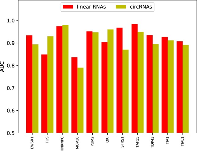
Comparison of AUCs for common RBPs shared by linear RNAs and circRNAs, in which the AUCs for linear RNAs and circRNAs are both obtained by CRIP using sequence information.
TABLE 2.
Some common motifs shared by circRNAs and linear RNAs
CRIP is able to detect RBP-binding sites on full-length circRNAs
In this section, we assess the capability of CRIP for predicting RBP-binding sites on full-length circRNAs. For each RBP, we randomly select 20 circRNAs with full-length sequences, half of which are bound to the RBP and half are not. Because the training and test sequences of CRIP are 101-bp segments, when testing for a new circRNA, we first segment the whole sequence into segments without overlap, and then we predict the binding potential for each segment to determine whether the segment contains a binding site or not. Therefore, all the 740 (37 × 20) circRNAs are segmented into fragments of length 101 (these fragments have been removed from the training set). CRIP outputs a probability of being a binding site for each segment. Then the output probabilities of all segments are averaged for each circRNA. To assess the performance of CRIP, we compute the Pearson correlation score between the average probability obtained by CRIP and the true probability for a segment being a binding site
on the circRNA. The correlation scores are listed in Supplemental Table S2. The score averaged over 37 RBP data sets is 0.48, and 10 of them are >0.8, showing a strong positive correlation between the predicted probability and the true probability. Generally, the higher the percentage of the segments predicted to be bound by the given RBP, the more chances this circRNA will interact with the RBP.
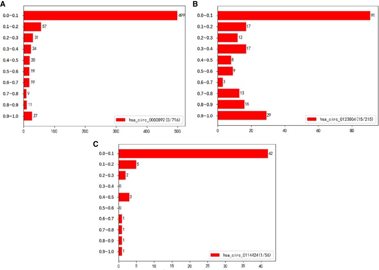
Take the RBP AUF1 as an example. Given the model trained for AUF1, the test results of CRIP on three circRNAs—hsa_circ_0000892, hsa_circ_0123804, and hsa_circ_0114424—are shown in Figure 8. They have very different lengths and are segmented into 716, 215, and 56 fragments of length 101 without overlap, respectively. According to the circRNA Interactome database (Dudekula et al. 2016), hsa_circ_0000892 has no segment binding to AUF1, whereas hsa_circ_0123804 and hsa_circ_0114424 have 15 and one segments binding to AUF1, respectively. As for hsa_circ_0123804, which has a close interaction with AUF1, many more segments are assigned with high probabilities compared with two other circRNAs. Using the default threshold (0.5) of classification, the false-positive percentages of hsa_circ_0000892 and hsa_circ_0114424 are 11.9% (85/716) and 5.4% (3/56), respectively. If using a higher cutoff, we can get a much lower false-positive rate. A major reason for the false positives is the procedure of training data generation.
FIGURE 8.
Prediction probability distributions on full-length circRNAs. The numbers before and after “/” denote the number of positive segments and the total number of segments, respectively.
Following the practice of previous studies, when preparing the training and test data sets of CRIP, we segment the original sequences of circRNAs into pieces of length 101. The segments containing the peaks of CLIP-seq reads are regarded as positive samples, and the negative samples are randomly selected from the remaining segments. The positive-to-negative ratio is 1:1, whereas the binding sites on RNA sequences are very rare (i.e., there are many more negative samples than positive samples). CRIP can provide a helpful prediction on whether or not the given circRNA and RBP interact and also the specific binding sites. A future development direction of CRIP is to reduce the false-positive rate when handling full-length circRNAs.
DISCUSSION
The stacked codon encoding versus random encoding
The success of CRIP lies in the enriched feature representation and powerful deep learning model. The coding potential of circRNAs inspired us to develop a codon-based encoding method. Although most circRNAs are still noncoding, the codon-based encoding outperforms the classic one-hot encoding by a large margin. A major reason is the expanded feature space, as the classic one-hot has only four symbols, whereas the codon-based encoding has 21 symbols.
Unlike the conventional one-hot method which encodes nucleotides one by one, the new encoding method traverses the 3-mers sequentially in an overlapping manner, just like the traditional k-mer feature extraction. Then, it encodes the 3-mers into binary vectors according to the codons for amino acids. Benefiting from the context information retained in the 3-mers and the expanded feature space, the new codon-based encoding method produces more informative representations.
The codons provide us a guideline on how to design the symbols and their corresponding triplets. Actually, the combinations of nucleotides can be arbitrarily mapped to a new alphabet, thus resulting in a new encoding scheme. To demonstrate the superiority of the codon-based mapping over random mappings, we construct six random encoding systems for comparison. The first three systems have the same number of symbols (21) as the codon-based encoding, whereas the other three systems have 10 symbols (i.e., a greater reduction on the original 3-mer space). Supplemental Table S3 shows the average AUCs across 10 RBP data sets of the seven encoding systems. Generally, the 10-symbol encoding methods perform worse than 21-symbol methods, suggesting that further reduction of the encoded feature space may hurt the discrimination accuracy. Among the seven encoding schemes, the codon-based method performs the best. Especially, we find that the codon-based method has more advantage on the data sets with low prediction accuracy. For example, on ALKBH5, the AUC obtained by codon-based encoding is 0.771, whereas the highest AUC by other systems is only 0.688. The experimental results demonstrate that the 3-nt combinations defined by codons are superior to random combinations defined in other encoding systems.
Motif analysis
To further explore the sequence patterns of RBP-binding sites on circRNAs, we search motifs from the positive sequence fragments using the MEME suite (Bailey et al. 2009). The motifs are extracted for each RBP data set, and the most significant motif of each RBP is shown in Supplemental Table S4, in which the width of motifs ranges from 8 to 15. As mentioned earlier in the subsection “Linear RNAs and circRNAs binding to the same RBPs differ in the prediction accuracy,” we find that some circRNAs have the same motifs as linear RNAs when binding to the same RBPs, indicating the two types of RNAs may share a common binding mechanism. We also find that the binding sites for some RBPs exhibit a common pattern (i.e., “GAAGAAG”), including AGO2, ALKBH5, CAPRIN1, LIN28B, and IGF2BP3. Actually, it is a common motif related to RNA modification (Dominissini et al. 2016; Li et al. 2016).
Despite the common motifs, for the same RBP, binding sites on circRNAs and linear RNAs may have large sequence diversity. A typical example is the circRNAs and linear RNAs binding to FUS. The model trained on linear RNAs has a very low prediction accuracy on circRNAs (Fig. 6), whereas when using CRIP trained on circRNAs, the accuracy becomes much higher than that of linear RNAs. Therefore, it would be interesting to explore the different binding mechanisms that lead to performance variance.
Limitations and potential applications of CRIP
CRIP is an RBP-specific model because the binding preference of individual RBPs is specific. Thus, for an RBP not in the trained models, CRIP cannot be directly used to predict circRNA targets for this RBP. However, if this RBP has homologous RBPs in the trained models, the trained model of its homologous RBP might be used to predict targets for this RBP.
There exist some potential applications of CRIP. RBPs have been discovered to play important roles in circRNA production. To identify those RBPs related to circNRA biogenesis, we need to first predict the interactions between circRNAs and all available RBPs. As some RBPs—for example, FUS (Errichelli et al. 2017) and QKI (Conn et al. 2015)—have been experimentally verified to be involved in circRNA biogenesis, through the analysis on the binding sequence patterns from these verified interactions, we can identify novel RBPs involved in circRNA biogenesis.
Conclusion
This study aims to identify circRNA–protein interactions by using a machine learning model. By treating the task as a binary classification problem, we propose a new sequence encoding scheme and a hybrid neural network model. The idea of the new encoding method is to convert RNA triplets into pseudo–amino acids based on nucleotide codons in an overlapping manner and represent the pseudo–amino acids via one-hot encoding. And the hybrid neural network consists of a CNN module and a BiLSTM module. The goal of using a hybrid model is to combine the advantages of both the deep architectures and obtain better high-level abstraction features for the classification. The results show that both the new sequence encoding method and the hybrid model contribute to the performance improvement. Compared to the existing predictors, our model has an advantage in the prediction accuracy. We believe that this tool will contribute to uncovering functions of circRNAs.
MATERIALS AND METHODS
Data preparation
To assess the prediction performance of CRIP, we construct a benchmark set of RBP-binding sites on circRNAs. The bound sequences are extracted from the circRNA Interactome database (https://circinteractome.nia.nih.gov/), which houses more than 120,000 human circRNA sequences (Dudekula et al. 2016). Considering that our model is based solely on circRNA sequences and that a high sequence similarity may cause biased results for machine learning methods, we use the CD-HIT package (Fu et al. 2012) with a threshold of 0.8 to eliminate redundant sequences. Finally, we have a total of 32,216 circRNAs associated with 37 RBPs.
For each RBP, we build a classification model, in which the positive samples are derived from verified binding sites on circRNAs. Following our previous work (Pan and Shen 2017), from each binding site corresponding to the CLIP-seq read peak, we extract a 101-bp segment by extending 50 nt upstream and 50 nt downstream from the center of the binding site. The negative samples are extracted from the remaining fragments of the circRNAs, with the same length as positive samples. To examine the impact of segment length, we experiment with two other lengths, namely, 201-bp and 501-bp. We find that longer fragments lead to an obvious drop in the prediction accuracy. Generally, the longer the fragment, the more decrease in the accuracy. There are two potential reasons: (i) The model is unable to handle very long sequences because of the nature of the LSTM; and (ii) long segments contain much noise. According to our statistics of the data sets, the average length of the known binding sites on circRNA sequences is 47, and most of them are shorter than 101. Thus, 101 is a proper choice. The longer segments (e.g., 201- or 501-bp) may contain a large proportion of nonbinding nucleotides, which may distract learning the informative features from binding sites.
The positive samples and negative samples are filtered to remove redundant sequences with a cutoff of 0.8 using CD-HIT. The positive-to-negative ratio is 1:1, and the detailed data statistics are listed in Supplemental Table S5.
In addition, because CRIP is also applicable to linear RNAs, we compare the performance of CRIP with the existing tools on the prediction of interactions between linear RNAs and RBPs, using previously published benchmark sets of linear RNAs—that is, the same data set used in iONMF (Stražar et al. 2016) and iDeep (Pan and Shen 2017), retrieved from DoRiNA (Blin et al. 2015) and iCount (http://icount.biolab.si/). There are 31 data sets derived from CLIP-seq data, corresponding to 31 experiments and covering 19 RBPs. The positive and negative samples are generated in the same way as described above, and each of the 31 data sets has 5000 training samples and 1000 test samples.
Stacked codon–based encoding
Let S be an RNA sequence of a length L. It will be converted into a pseudo–amino acid sequence, whose alphabet is A = {A, C, D, E, F, G, H, I, K, L, M, N, P, Q, R, S, T, V, W, Y, Z}, where Z denotes the stop codon. S is represented by a 21 × (L − 2)-D matrix M (there are a total of L − 2 overlapping codons for a sequence of the length L). The jth column of the matrix is a one-hot vector for the jth letter in the converted sequence S′, where . Then the elements of M are represented by
| (1) |
where is the jth character of S′, denotes the index of in the alphabet A, and .
As illustrated in Figure 1, the corresponding pseudo–amino acid sequence of the input sequence GAGUAA is ESVZ, where GAG codes for E, AGU codes for S, GUA codes for V, and UAA is a stop codon. Because the indexes of E, S, V, and Z in the alphabet are 4, 16, 18, and 21, respectively, the generated matrix M is 21 × (L − 2)-D, and M4, 1, M16, 2, M18, 3, and M21, 4 are equal to 1, and other elements are zero.
The CNN layers
The CNN has been demonstrated to have a powerful capability to extract high-level abstract features, not only for image processing but also for natural language processing tasks (Yin et al. 2017). In this study, we also use a CNN as a feature extractor, whose input is the sequence encoding (i.e., the matrix M described in the previous subsection). Assume the size of M is d × l, where d is the dimensionality of the one-hot vectors (d = 21 for the stacked codon–based encoding) and l is the length of the converted pseudo–amino acid sequence. We take a one-dimensional convolution along the sequence. For the convolutional layer, we set the length of a filter as hf, which means that the filters are operated on hf words/tokens. Let Xi be the original encoding matrix for the segment of the input sequence processed by the sliding kernels at the ith time step, which is actually a submatrix of M, consisting of the ith to (i + hf − 1)th columns of M. For convenience, we take the transposed submatrix of M as Xi. Then the size of Xi is (i + hf − 1) × d. The corresponding outputs of all Xi passing through the jth sliding kernel turns out to be a column vector yj. Each element, is defined as
| (2) |
where g(·) is an ReLU function, n is the number of the filters, W is the convolutional filter (), and b is the bias. In the pooling layer, we choose an average pooling over the sequence with the length of hp. The output of the pooling layer for the jth filter is a column vector defined as zj, where the mth element is computed by
| (3) |
Let Z be the matrix whose column vectors are zj (i.e., the high-level features learned by the CNN model). Z is fed to the subsequent BiLSTM model for classification.
The BiLSTM layer
Through the convolutional filters and average pooling layers, the CNN module learns and integrates local information of RNA sequences. Then we stitch the data of all the channels of each subunit into a new feature vector. To further exploit the sequence information, we adopt a bidirectional long- and short-term memory network (BiLSTM). Compared with traditional recurrent neural networks (RNNs), LSTM has advantages in addressing the vanishing/exploding gradient problem and long-term dependency. In particular, BiLSTM exploits the contextual information on both sides. Let st and be the hidden states for the forward and backward computation at the tth time step. The calculation of st and relies on st−1 and , respectively, as defined in Eqs. (4) and (5):
| (4) |
where U and W are the weight matrices for the input and the hidden state, respectively, and zt is the input vector in the tth step(i.e., the tth row vector of Z), and
| (5) |
where U′ and W′ are the weight matrices for the input and the hidden state used in the backward computation, respectively. To integrate contextual information, the output for tth step is defined as
| (6) |
where V and V′ are the transformation matrices of the preceding and following context for the current time step.
Output concatenation and the fully connected layers
By convention, only the outputs of the last LSTM are fed to the fully connected layer for final classification. In this study, we find that the outputs of previous time steps also contain some informative signals for the classification. Therefore, we concatenate the output vectors of all the time points:
| (7) |
In addition, because the concatenated output has a high dimensionality, we add two fully connected layers to gradually reduce the dimensionality for the final classification, and the softmax layer maps all outputs to probabilities:
| (8) |
| (9) |
| (10) |
where g is the ReLU function, and are the weight matrices, and and are the bias terms.
Experimental settings
In CRIP, the convolution layers have 102 filters of size 7 × 21, and the kernel size is fixed to be 7. We also test different sizes (i.e., 3, 5, 9, 11) and a combination of kernels. The kernel size 7 yields a slightly higher AUC than other kernel sizes, and the combination of kernels performs a little bit better than the single-kernel methods, whereas the performance difference is not significant (Supplemental Table S6). In this model, different kernels of the CNN may extract similar high-level features and their combination may obtain redundant features. The kernel size 7 is a moderate size for extracting features from RNA sequences.
For each data set, we extract 20% of the data as the test set and adopt fivefold cross-validation within the training set to select parameters. The batch size 50 and training epoch number 30 achieve the optimum results. The source code and data sets are available at https://github.com/kavin525zhang/CRIP.
SUPPLEMENTAL MATERIAL
Supplemental material is available for this article.
Supplementary Material
ACKNOWLEDGMENTS
This work was supported by the National Key Research and Development Program of China (no. 2018YFC0910500), the National Natural Science Foundation of China (nos. 61972251, 61725302, 61671288, 61603161), and the Science and Technology Commission of Shanghai Municipality (nos. 16ZR1448700, 16JC1404300, 17JC1403500).
Footnotes
Article is online at http://www.rnajournal.org/cgi/doi/10.1261/rna.070565.119.
Because circRNAs only have sequence information, we retrain the iDeep (Pan and Shen 2017) using linear RNA sequence information alone and name it iDeep*.
REFERENCES
- Alipanahi B, Delong A, Weirauch MT, Frey BJ. 2015. Predicting the sequence specificities of DNA- and RNA-binding proteins by deep learning. Nat Biotechnol 33: 831 10.1038/nbt.3300 [DOI] [PubMed] [Google Scholar]
- Bailey TL, Boden M, Buske FA, Frith MC, Grant CE, Clementi L, Noble WS. 2009. MEME Suite: tools for motif discovery and searching. Nucleic Acids Res 37: 202–208. 10.1093/nar/gkp335 [DOI] [PMC free article] [PubMed] [Google Scholar]
- Baldi P, Brunak S, Stolovitzky GA. 2002. Bioinformatics: the machine learning approach. Phys Today 55: 57–58. 10.1063/1.2408440 [DOI] [Google Scholar]
- Blin K, Dieterich C, Wurmus R, Rajewsky N, Landthaler M, Akalin A. 2015. DoRiNA 2.0–upgrading the doRiNA database of RNA interactions in post-transcriptional regulation. Nucleic Acids Res 43: 160–167. 10.1093/nar/gku1180 [DOI] [PMC free article] [PubMed] [Google Scholar]
- Chen W, Lei TY, Jin DC, Lin H, Chou KC. 2014. PseKNC: a flexible web server for generating pseudo k-tuple nucleotide composition. Anal Biochem 456: 53–60. 10.1016/j.ab.2014.04.001 [DOI] [PubMed] [Google Scholar]
- Conn SJ, Pillman K, Toubia J, Conn V, Salmanidis M, Phillips CA, Roslan S, Schreiber AW, Gregory PA, Goodall GJ. 2015. The RNA binding protein quaking regulates formation of circRNAs. Cell 160: 1125–1134. 10.1016/j.cell.2015.02.014 [DOI] [PubMed] [Google Scholar]
- Cornishbowden A. 1985. Nomenclature for incompletely specified bases in nucleic acid sequences: recommendations 1984. Nucleic Acids Res 150: 1–5. [DOI] [PMC free article] [PubMed] [Google Scholar]
- Dominissini D, Nachtergaele S, Moshitch-Moshkovitz S, Peer E, Kol N, Ben-Haim MS, Dai Q, Segni AD, Salmondivon M, Clark WC, et al. 2016. The dynamic N1-methyladenosine methylome in eukaryotic messenger RNA. Nature 530: 441 10.1038/nature16998 [DOI] [PMC free article] [PubMed] [Google Scholar]
- Du WW, Yang W, Chen Y, Wu Z, Foster FS, Yang Z, Yang BB. 2016. Foxo3 circular RNA promotes cardiac senescence by modulating multiple factors associated with stress and senescence responses. Eur Heart J 38: 1402–1412. 10.1093/eurheartj/ehw001 [DOI] [PubMed] [Google Scholar]
- Dudekula DB, Panda AC, Grammatikakis I, De S, Abdelmohsen K, Gorospe M. 2016. Circinteractome: a web tool for exploring circular RNAs and their interacting proteins and microRNAs. RNA Biol 13: 34–42. 10.1080/15476286.2015.1128065 [DOI] [PMC free article] [PubMed] [Google Scholar]
- Errichelli L, Dini Modigliani S, Laneve P, Colantoni A, Legnini I, Capauto D, Rosa A, Santis RD, Scarfo R, Peruzzi G, et al. 2017. FUS affects circular RNA expression in murine embryonic stem cell-derived motor neurons. Nat Commun 8: 14741 10.1038/ncomms14741 [DOI] [PMC free article] [PubMed] [Google Scholar]
- Fan C, Lei X, Fang Z, Jiang Q, Wu FX. 2018. CircR2Disease: a manually curated database for experimentally supported circular RNAs associated with various diseases. Database 2018: bay044 10.1093/database/bay044 [DOI] [PMC free article] [PubMed] [Google Scholar]
- Fu L, Niu B, Zhu Z, Wu S, Li W. 2012. CD-HIT. Bioinformatics 28: 3150–3152. 10.1093/bioinformatics/bts565 [DOI] [PMC free article] [PubMed] [Google Scholar]
- Glažar P, Papavasileiou P, Rajewsky N. 2014. Circbase: a database for circular RNAs. RNA 20: 1666–1670. 10.1261/rna.043687.113 [DOI] [PMC free article] [PubMed] [Google Scholar]
- Hansen TB, Kjems J, Damgaard CK. 2013a. Circular RNA and mir-7 in cancer. Cancer Res 73: 5609–5612. 10.1158/0008-5472.CAN-13-1568 [DOI] [PubMed] [Google Scholar]
- Hansen TB, Jensen TI, Clausen BH, Bramsen JB, Finsen B, Damgaard C, Kjems J. 2013b. Natural RNA circles function as efficient microRNA sponges. Nature 495: 384–388. 10.1038/nature11993 [DOI] [PubMed] [Google Scholar]
- Jeck WR, Sorrentino JA, Wang K, Slevin MK, Burd CE, Liu J, Marzluff WF, Sharpless NE. 2013. Circular RNAs are abundant, conserved, and associated with Alu repeats. RNA 19: 141–157. 10.1261/rna.035667.112 [DOI] [PMC free article] [PubMed] [Google Scholar]
- Johnson AD. 2010. An extended IUPAC nomenclature code for polymorphic nucleic acids. Bioinformatics 26: 1386–1389. 10.1093/bioinformatics/btq098 [DOI] [PMC free article] [PubMed] [Google Scholar]
- Li JH, Liu S, Zhou H, Qu LH, Yang JH. 2013. starBase v2.0: decoding miRNA-ceRNA, miRNA-ncRNA and protein-RNA interaction networks from large-scale CLIP-Seq data. Nucleic Acids Res 42: D92–D97. [DOI] [PMC free article] [PubMed] [Google Scholar]
- Li Y, Zheng Q, Bao C, Li S, Guo W, Zhao J, Chen D, Gu J, He X, Huang S. 2015. Circular RNA is enriched and stable in exosomes: a promising biomarker for cancer diagnosis. Cell Res 25: 981–984. 10.1038/cr.2015.82 [DOI] [PMC free article] [PubMed] [Google Scholar]
- Li X, Xiong X, Wang K, Wang L, Yi C. 2016. Transcriptome-wide mapping reveals reversible and dynamic N1-methyladenosine methylome. Nat Chem Biol 12: 311 10.1038/nchembio.2040 [DOI] [PubMed] [Google Scholar]
- Li B, Zhang X, Liu S, Liu S, Sun W, Lin Q, Luo YX, Zhou KR, Zhang CM, Tan YY, et al. 2017a. Discovering the interactions between circular RNAs and RNA-binding proteins from CLIP-seq data using circScan. bioRxiv 115980 10.1101/115980 [DOI] [Google Scholar]
- Li YE, Xiao M, Shi B, Yang YC, Wang D, Wang F, Marcia M, Lu ZJ. 2017b. Identification of high-confidence RNA regulatory elements by combinatorial classification of RNA–protein binding sites. Genome Biol 18: 169 10.1186/s13059-017-1298-8 [DOI] [PMC free article] [PubMed] [Google Scholar]
- Memczak S, Jens M, Elefsinioti AL, Torti F, Krueger J, Rybak A, Maier L, Mackowiak SD, Gregersen LH, Munschauer M, et al. 2013. Circular RNAs are a large class of animal RNAs with regulatory potency. Nature 495: 333–338. 10.1038/nature11928 [DOI] [PubMed] [Google Scholar]
- Muppirala UK, Honavar VG, Dobbs D. 2011. Predicting RNA-protein interactions using only sequence information. BMC Bioinformatics 12: 489 10.1186/1471-2105-12-489 [DOI] [PMC free article] [PubMed] [Google Scholar]
- Pamudurti NR, Bartok O, Jens M, Ashwal-Fluss R, Stottmeister C, Ruhe L, Hanan M, Wyler E, Perezhernandez D, Ramberger E, et al. 2017. Translation of circRNAs. Mol Cell 66: 9–21. 10.1016/j.molcel.2017.02.021 [DOI] [PMC free article] [PubMed] [Google Scholar]
- Pan X, Shen HB. 2017. RNA-protein binding motifs mining with a new hybrid deep learning based cross-domain knowledge integration approach. BMC Bioinformatics 18: 136 10.1186/s12859-017-1561-8 [DOI] [PMC free article] [PubMed] [Google Scholar]
- Pan X, Shen HB. 2018. Predicting RNA-protein binding sites and motifs through combining local and global deep convolutional neural networks. Bioinformatics 34: 3427–3436. 10.1093/bioinformatics/bty364 [DOI] [PubMed] [Google Scholar]
- Pan X, Rijnbeek P, Yan J, Shen HB. 2018. Prediction of RNA-protein sequence and structure binding preferences using deep convolutional and recurrent neural networks. BMC Genomics 19: 511 10.1186/s12864-018-4889-1 [DOI] [PMC free article] [PubMed] [Google Scholar]
- Park S, Min S, Choi H, Yoon S. 2017. Deep recurrent neural network-based identification of precursor microRNAs. Adv Neural Inf Process Syst 2017: 2891–2900. [Google Scholar]
- Ray D, Kazan H, Cook KB, Weirauch MT, Najafabadi HS, Li X, Gueroussov S, Albu M, Zheng H, Yang A, et al. 2013. A compendium of RNA-binding motifs for decoding gene regulation. Nature 499: 172–177. 10.1038/nature12311 [DOI] [PMC free article] [PubMed] [Google Scholar]
- Shen J, Zhang J, Luo X, Zhu W, Yu K, Chen K, Li YX, Jiang HL. 2007. Predicting protein–protein interactions based only on sequences information. Proc Natl Acad Sci 104: 4337–4341. 10.1073/pnas.0607879104 [DOI] [PMC free article] [PubMed] [Google Scholar]
- Stražar M, Žitnik M, Zupan B, Ule J, Curk T. 2016. Orthogonal matrix factorization enables integrative analysis of multiple RNA binding proteins. Bioinformatics 32: 1527–1535. 10.1093/bioinformatics/btw003 [DOI] [PMC free article] [PubMed] [Google Scholar]
- Van Nostrand EL, Pratt GA, Shishkin AA, Gelboin-Burkhart C, Fang MY, Sundararaman B, Blue SM, Nguyen TB, Surka C, Elkins K, et al. 2016. Robust transcriptome-wide discovery of RNA-binding protein binding sites with enhanced clip (eCLIP). Nat Methods 13: 508 10.1038/nmeth.3810 [DOI] [PMC free article] [PubMed] [Google Scholar]
- Wang Y, Mo Y, Gong Z, Yang X, Yang M, Zhang S, Xiong F, Xiang B, Zhou M, Liao QZ, et al. 2017. Circular RNAs in human cancer. Mol Cancer 16: 25 10.1186/s12943-017-0598-7 [DOI] [PMC free article] [PubMed] [Google Scholar]
- Xia S, Feng J, Lei L, Hu J, Xia L, Wang J, Xiang Y, Liu LJ, Zhong S, Han L, et al. 2016. Comprehensive characterization of tissue-specific circular RNAs in the human and mouse genomes. Brief Bioinform 18: 984–992. 10.1093/bib/bbw081 [DOI] [PubMed] [Google Scholar]
- Yan J, Friedrich S, Kurgan L. 2016. A comprehensive comparative review of sequence-based predictors of DNA-and RNA-binding residues. Brief Bioinform 17: 88–105. 10.1093/bib/bbv023 [DOI] [PubMed] [Google Scholar]
- Yin W, Kann K, Mo Y, Schütze H. 2017. Comparative study of CNN and RNN for natural language processing. arXiv 1702.01923. [Google Scholar]
- Zhang T, Zhang H, Chen K, Ruan J, Shen S, Kurgan L. 2010. Analysis and prediction of RNA-binding residues using sequence, evolutionary conservation, and predicted secondary structure and solvent accessibility. Curr Protein Pept Sci 11: 609–628. 10.2174/138920310794109193 [DOI] [PubMed] [Google Scholar]
- Zhang Y, Wang X, Kang L. 2011. A k-mer scheme to predict piRNAs and characterize locust piRNAs. Bioinformatics 27: 771–776. 10.1093/bioinformatics/btr016 [DOI] [PMC free article] [PubMed] [Google Scholar]
Associated Data
This section collects any data citations, data availability statements, or supplementary materials included in this article.


