Resting state connectivity differences in eyes open versus eyes closed conditions

Abstract

Functional magnetic resonance imaging data are commonly collected during the resting state. Resting state functional magnetic resonance imaging (rs‐fMRI) is very practical and applicable for a wide range of study populations. Rs‐fMRI is usually collected in at least one of three different conditions/tasks, eyes closed (EC), eyes open (EO), or eyes fixated on an object (EO‐F). Several studies have shown that there are significant condition‐related differences in the acquired data. In this study, we compared the functional network connectivity (FNC) differences assessed via group independent component analysis on a large rs‐fMRI dataset collected in both EC and EO‐F conditions, and also investigated the effect of covariates (e.g., age, gender, and social status score). Our results indicated that task condition significantly affected a wide range of networks; connectivity of visual networks to themselves and other networks was increased during EO‐F, while EC was associated with increased connectivity of auditory and sensorimotor networks to other networks. In addition, the association of FNC with age, gender, and social status was observed to be significant only in the EO‐F condition (though limited as well). However, statistical analysis did not reveal any significant effect of interaction between eyes status and covariates. These results indicate that resting‐state condition is an important variable that may limit the generalizability of clinical findings using rs‐fMRI.

1. INTRODUCTION

Resting state functional magnetic resonance imaging (rs‐fMRI) is a data collection method that does not require participants to engage in a specific task. This allows rs‐fMRI to be acquired from a wide range of populations including patient groups, participants with intellectual disabilities, pediatric groups, and even unconscious patients (Smitha et al., 2017). Since Biswal, Yetkin, Haughton, and Hyde (1995) initially observed that temporal correlation of low frequency fluctuations in rs‐fMRI (<0.1 Hz) can provide an estimate of functional connectivity (FC), research on rs‐fMRI has greatly increased (Agcaoglu et al., 2018; Agcaoglu, Miller, Mayer, Hugdahl, & Calhoun, 2016; Allen et al., 2011; Cetin et al., 2016; Haak, Marquand, & Beckmann, 2018; Hart et al., 2018; Park, Friston, Pae, Park, & Razi, 2018; Rashid et al., 2018; Smitha et al., 2017).

Rs‐fMRI is commonly scanned in at least one of three different conditions, eyes closed (EC), eyes open (EO), and eyes fixated on a target (EO‐F), usually a crosshair. In the EC case, participants are asked to closed their eyes and stay awake during the scanning; in the EO case, the participants are asked to keep their eyes open; and in the EO‐F case, the participants are asked to keep their eyes fixated on an object, usually a crosshair presented at the center of the screen, during scanning. Several previous studies have focused on the difference in fMRI assessed brain activation during these scanning conditions. For example, Patriat et al. (2013) analyzed FC differences in EC, EO, and EO‐F conditions as well as reliability and consistency between multiple scans of the same scanning conditions; they found higher FC in auditory networks in EC condition and greater reliability in EO‐F condition in default‐mode, attention and auditory networks; and greater reliability in visual networks in EO conditions. Liu, Dong, Zuo, Wang, and Zang (2013) evaluated split half reproducibility for EO and EC conditions using three metrics including amplitude of low frequency fluctuations, regional homogeneity and seed‐based correlation, and found that reproducible patterns of EO‐EC differences can be detected in all three measures. Yan et al. (2009) found significantly higher FC in default‐mode network (DMN) in both EO and EO‐F conditions compared to EC. Van Dijk et al. (2010) found significantly higher FC in DMN and attentional networks for EO‐F case compared to EC, but they did not find any significant differences when comparing EO‐F and EO conditions. There have been a few studies analyzing functional network connectivity (FNC) utilizing group independent component analysis (gICA) on the same small EEG‐fMRI dataset (25 participants); Wu, Eichele, and Calhoun (2010) found higher FNC in EO case, compared to EC case, and Allen, Damaraju, Eichele, Wu, and Calhoun (2018) investigated dynamic FNC states for EO versus EC conditions, found association between dynamic connectivity in concurrently collected EEG and fMRI data and a large effect of vigilance on FNC.

In this study, we investigated FNC differences between EO‐F and EC cases on a large fMRI dataset (173 participants) of children scanned via a multiband sequence with a short sampling rate. This study makes three key contributions: first, to our knowledge, this is the only study that compares these resting state conditions in such a large dataset. Second, we investigate the effects of various covariates (e.g., age, gender, and social status score) on EO‐F and EC cases. Third, we perform a comprehensive (whole brain) analysis of connectivity using gICA and FNC between all pairs of brain networks.

2. METHODS AND MATERIALS

2.1. Participants

In this study, we used resting state fMRI scans of EO‐F and EC conditions collected from 182 participants from two different sites (Mind Research Network [MRN]/New Mexico and University of Nebraska Medical Center/Nebraska). Participants were asked to stare at a fixation cross during the eyes open scanning and to close their eyes but remain awake during the eyes closed condition. Initially, 358 different scans were used in the gICA state. We removed participants who had only EO‐F or EC scans available, resulting in 346 scans from 173 participants (age range from 9.1 to 15.5 years, 11.95 ± 1.78). The included participant had maximum mean frame displacement (MFD) of 0.3 mm, and mean of MFD was 0.074 mm with a standard deviation of 0.03 mm. Demographic information of the subjects was summarized in Table 1.

Table 1.

Demographic information of the participants, the dataset included 173 subjects (89 males) with age range 9.1–15.5 years old

	# of subjects		%
Gender	173		100
Male	89		51.45
Female	84		48.55
Age (years)	Mean	SD	Min	Max
Male	12.03	1.88	9.1	15.5
Female	11.89	1.66	9.2	15.1

2.2. Imaging parameters

Imaging data at the MRN site were collected on a 3T Siemens Tim Trio scanner and a 3T Siemens Skyra scanner was used at the Nebraska site. A total of 650 volumes of echo planar imaging BOLD data were collected per condition and participant with a TR of 0.46 s, TE = 29 ms, FA = 44°, and a slice thickness of 3 mm with no gap. Rs‐fMRI scans were acquired using a standard gradient‐echo echo planar imaging paradigm; MRN site: FOV of 246 × 246 mm (82 × 82 matrix), 56 sequential axial slices; Nebraska: FOV of 268 × 268 mm (82 × 82 matrix), 48 sequential axial slices. The order of the EO‐F and EC sessions were counter‐balanced across participants at each site.

2.3. Preprocessing

The data were preprocessed using a combination of toolboxes (AFNI, http://afni.nimh.nih.gov, SPM, http://www.fil.ion.ucl.ac.uk/spm, GIFT, http://mialab.mrn.org/software/gift), and custom scripts written in MATLAB. Rigid body motion correction was performed using the INRIAlign (Freire & Mangin, 2001) toolbox in SPM to correct for subject head motion followed by slice‐timing correction to account for timing differences in slice acquisition. Then the fMRI data were despiked using 3dDespike algorithm in AFNI (https://afni.nimh.nih.gov) to mitigate the impact of outliers. The fMRI data were subsequently warped to a Montreal Neurological Institute (MNI) template (http://www.mni.mcgill.ca) and resampled to 3 mm³ isotropic voxels, the first four volumes of each session were discarded to account for the T1 equilibrium effect. Because participants consisted of children with an age range of 9.1–15.5, we rewarped the data to a study specific template computed as the average of the first time point from each scan. Next we smoothed the data to 6 mm full width at half maximum (FWHM).

2.4. Group independent component analysis

The preprocessed functional data was analyzed with gICA implemented in the GIFT software (Calhoun & Adali, 2012; Calhoun, Adali, Pearlson, & Pekar, 2001; Calhoun, Adali, Pearlson, & Pekar, 2002) and decomposed into 150 spatially independent components. Prior to gICA, a scan specific principle component analysis (PCA) was applied to reduce the dimensionality across the 646 time points to 200 maximally variable directions. The reduced data were concatenated across time and a group PCA was applied to further reduce the dimensionality to 150 (Erhardt et al., 2011). One hundred and fifty independent components were estimated from the group PCA reduced matrix using the infomax algorithm (Bell & Sejnowski, 1995). We repeated the ICA algorithm 20 times in ICASSO (Himberg, Hyvarinen, & Esposito, 2004; http://www.cis.hut.fi/projects/ica/icasso) to ensure stability of the estimation, and the most central run was selected from the resulting 20 runs (Ma et al., 2011). A spatially constrained ICA algorithm (Du et al., 2016; Du & Fan, 2013) was used to estimate subject specific spatial maps (SMs) and time courses (TCs) from the group maps, called group information guided ICA (GIG‐ICA) as implemented in the GIFT software.

2.5. Post‐gICA processing

Subject specific SMs and TCs were postprocessed with methods similar to that described in a previous study (Allen et al., 2011). We calculated one sample t‐test maps for each SM across all participants and then thresholded these maps to obtain regions of peak connectivity for the corresponding component. We also computed mean power spectra of the corresponding TCs. Later, these components were analyzed based on criteria such as peak activated voxel location in gray matter, showing less overlap with known vascular, susceptibility, ventricular and edge regions corresponding to head motion by visually and using AFNI whereami function; and 51 components out of 150 were identified as the resting state networks (RSNs). These 51 RSNs were also grouped based on their anatomical and functional properties by visual observation and using AFNI whereami function; including 4 sub cortical networks (SC), 3 auditory networks (Aud), 8 sensorimotor networks (SM), 18 visual networks (Vis), 4 default‐mode networks (DMN), 12 cognitive control networks (CC), and 2 cerebellar networks (Cb).

The subject specific TCs were detrended, motion parameters were regressed (including their derivatives, their squares, and derivatives of their squares), and then despiked, which involved detecting spikes as determined by AFNI's 3dDespike algorithm and replacing spikes by values obtained from third order spline fit to neighboring clean portions of the data.

2.6. Functional network connectivity

FNC is a measure that shows the average FC among different RSNs during scanning, calculated as the pairwise correlation between RSN time courses. TCs were filtered using a fifth‐order Butterworth low‐pass filter with a high frequency cutoff of 0.15 Hz since correlation among brain networks is primarily driven by the low frequency fluctuations in BOLD fMRI data (Cordes et al., 2001). We calculated FNC matrix for each subject for eyes open and eyes closed cases separately, and averaged over subjects. We estimated covariance from the regularized precision matrix or the inverse covariance matrix (Smith et al., 2011). Following the graphical LASSO method of Friedman, Hastie, and Tibshirani (2008), we placed a penalty on the L1 norm of the precision matrix to promote sparsity. The regularization parameter lambda (λ) was optimized separately for each subject by evaluating the log‐likelihood of the unseen data in a cross‐validation framework. The unseen data was the windowed covariance matrices from the same subject, using a Gaussian window of size 323 with alpha parameter of 1. This resulted in a penalty parameter of 0.1 for all subjects, and final FNC were calculated using all 646 time courses. FNC matrix was initially organized similar to Allen et al. (2014) as the main modules of subcortical, auditory, sensorimotor, visual, default‐mode, cognitive control, and cerebellar. Then, we applied the Louvain algorithm from the brain connectivity toolbox https://sites.google.com/site/bctnet) to arrange the RSN ordering within these main modules.

2.7. Eyes open‐ eyes closed FNC differences

We compared the FNC differences between EO‐F and EC cases with a paired t‐test and corrected for multiple comparisons with false discovery rate (FDR) of 0.01. Before calculating the paired t‐test, we regressed out motion (as the mean frame displacement) to minimize any effect. We also confirmed there was no significant motion difference for EO‐F and EC cases (paired t‐test, p = 0.7443).

2.8. Effect of age, gender, and social status scores on FNCs

We analyzed how age, gender, and social status scores affected the network connectivity with a regression model and corrected for multiple comparison with FDR of 0.05. We also added site and mean frame displacements as nuisance covariates. Gender was coded as 1 for males and 0 for females. We applied this model to the EO‐F and EC cases separately. We used the Barratt simplified measure of social status, which was available for 156 subjects to measure social status.

3. RESULTS

3.1. Resting state networks

The gICA revealed 51 RSNs which were grouped based on their anatomical and functional properties, including 4 sub corticals (SC), 3 auditory (Aud), 8 sensorimotor (SM), 18 visual (Vis), 4 default‐mode networks (DMN), 12 cognitive control (CC), and 2 cerebellum (Cb). These networks are displayed in Figure 1 and corresponding anatomical regions and peak locations are presented in Table 2.

Figure 1.

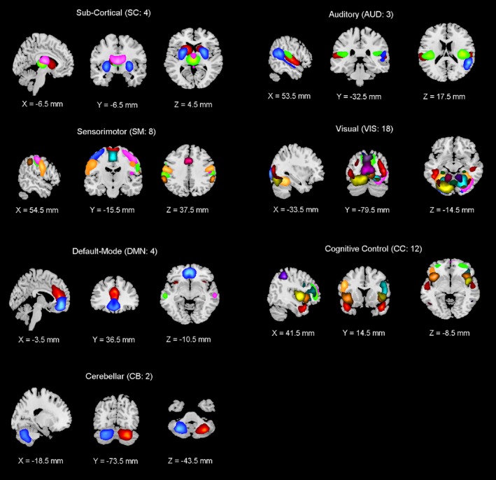
51 resting state components are presented as subgroups based on their anatomical and functional properties, including 4 sub‐cortical (SC), 3 auditory (Aud), 8 sensorimotor (SM), 18 visual (Vis), 4 default‐mode networks (DMN), 12 cognitive control (CC), and 2 cerebellum (Cb) [Color figure can be viewed at http://wileyonlinelibrary.com]

Table 2.

Anatomical regions associated with the RSNs presented in Figure 1 and MNI coordinates of the peaks. L = Left, R = Right, G = gyrus, Inf = Inferior, Temp = Temporal

IC#	Nv	Tmax	Coord.	BA
Sub‐Cortical Networks
85
L putamen	1,463	141.63	−18 10 4
R putamen	735	82.27	20 12 0
54
R putamen	1,224	135.54	26 4 −2
L putamen	1,197	147.24	−28 0 −2
58
R thalamus	1,033	170.69	2 −20 6
68
L thalamus	1,430	141.33	−4 −12 12
Auditory Networks
62
L superior Temp G	2,267	84.25	−52 −18 6	22
R superior Temp G	2,029	87.45	60 −12 0	22
145
R superior Temp G	3,713	104.6	56 −44 18	13
L middle Temp G	1,378	51.41	−58 −54 12	22
125
R insula lobe	1908	119.75	42 −18 12	13
L superior Temp G	1,795	107.6	−46 −24 12	41
Sensorimotor Networks
9
L paracentral lobule	2,599	94.33	0 −24 72	6
8
L postcentral G	1828	94.76	−46 −30 54	2
R postcentral G	383	37.47	54 −20 48	1
98
L Inf parietal lobule	2,438	96.03	−54 −30 46	2
R supramarginal G	1,621	76.73	60 −20 40	3
26
R postcentral G	2,515	96.98	44 −30 58	2
L postcentral G	507	37.30	−42 −38 60	40
2
L postcentral G	1,080	91.31	−54 −8 34	6
R postcentral G	1,014	90.70	60 −6 30	6
73
L paracentral lobule	4,219	125.8	0 −24 54	6
L rolandic operculum	157	40.96	−40 −26 18	13
124
L Inf parietal lobule	1,073	76.71	−58 −42 42	40
R supramarginal G	873	73.92	60 −38 40	40
77
L SMA	4,587	101.23	0 6 52	6
R insula lobe	516	53.27	48 10 −2	22
Visual Networks
131
L Inf Temp G	2,183	74.55	−52 −50 −12	37
R fusiform G	1,668	60.82	44 −30 −18	20
76
R calcarine G	2,756	81.86	18 −102 −2	18
34
L cuneus	3,412	82.78	2 −80 24	18
42
R fusiform G	1,510	72.64	32 −78 −14	19
L cerebellum	569	36.52	−40 −68 −20	19
71
L fusiform G	1920	77.93	−30 −56 −14	19
R fusiform G	1,422	69.95	30 −48 −18	37
91
R lingual G	4,008	91.16	24 −72 −12	19
111
L lingual G	2,891	109.15	0 −78 4	18
69
L cerebellum	1,662	143.19	−6 −50 −2	30
82
R cerebellum	1,674	142.59	8 −50 −2	30
70
L lingual G	2,152	76.07	−18 −86 −18	18
33
R calcarine G	3,313	115.61	8 −68 10	30
59
R lingual G	2,465	127.29	12 −56 10	30
L middle occipital G	293	41.29	−42 −80 30	19
130
R middle occipital G	3,229	97.50	38 −84 6	19
L middle occipital G	3,092	82.44	−36 −86 6	19
100
Cerebellar vermis	1,270	192.57	2 −42 4	29
129
Cerebellar vermis	1,448	140.21	6 −56 0
38
L precuneus	3,174	79.17	0 −66 58	7
R superior frontal G	241	32.07	30 4 60	6
37
L posterior cingulate cortex	2019	141.39	0 −54 30	31
L angular G	509	45.23	−52 −68 28	39
27
R middle cingulate cortex	2,693	88.57	−4 −24 28	23
L Inf parietal lobule	207	35.50	−36 −62 48	7
Default Mode Networks
123
R anterior cingulate cortex	4,398	118.94	2 42 10	32
R insula lobe	538	59.55	36 18 −12	47
49
L mid orbital G	2,941	115.46	0 48 −6	10
L middle Temp G	253	39.78	−58 −14 −18	21
90
L angular G	2,579	91.98	−52 −62 30	39
L middle frontal G	2,269	52.91	−42 18 46	8
101
R middle frontal G	2,450	57.54	30 18 54	8
R Inf parietal lobule	1892	99.84	54 −56 40	40
Cognitive Control Networks
83
L middle Temp G	2,105	93.39	−46 6 −30	21
R medial Temp pole	1,588	96.98	48 10 −26	21
114
L sup. Medial frontal G	3,955	103.29	0 60 22	10
L Temp pole	733	40.71	−36 22 −20	47
63
R middle frontal G	6,987	115.49	32 58 4	10
R Inf parietal lobule	72	26.70	50 −50 48	40
48
L sup. Medial frontal G	2,744	86.68	0 66 18	10
R cerebellum	77	31.19	48 −72 −38
120
L. inf. front. G. (P. triangularis)	4,236	91.65	−48 30 18	46
R. inf. front. G. (P. triangularis)	855	52.20	50 22 28	46
146
R. inf. front. G. (P. opercularis)	7,279	114.14	50 18 6	45
L insula lobe	590	46.17	−34 24 −2	13
119
L insula lobe	2,186	116.66	−40 18 −6	47
R insula lobe	1,381	88.71	44 16 −2	47
96
L Inf parietal lobule	3,989	78.25	−24 −72 46	7
L precentral G	711	47.22	−52 10 34	9
102
R Inf parietal lobule	3,397	82.40	44 −42 48	40
R. inf. front. G. (P. opercularis)	1,660	51.33	54 12 30	9
133
R rolandic operculum	2,745	102.29	54 4 4	22
L rolandic operculum	766	51.31	−54 0 4	22
55
R superior parietal lobule	3,916	71.19	18 −54 66	7
R cerebellum	106	33.04	26 −44 −48
136
L angular G	6,603	74.10	−52 −78 28	39
R middle occipital G	807	58.53	44 −78 34	19
Cerebellar Networks
84
R cerebellum	4,173	150.37	30 −68 −38
110
L cerebellum	3,906	126.64	−30 −66 −38

3.2. Eyes open eyes closed group differences

The FNCs for EO‐F and EC cases are displayed in Figure 2 as one sample t‐statistics and thresholded with 0.01 levels FDR. Both FNC matrices show similar patterns; SC‐SC, Aud‐Aud, Vis‐Vis, DMN‐DMN, and Cb‐Cb domains were almost entirely positively correlated with Vis‐Vis having the highest correlation. CC‐CC showed both anti‐correlated and correlated networks. Vis‐SM and Vis‐Aud networks showed different patterns; for EO‐F these networks were mostly anti‐correlated, while they were mostly correlated in EC case. Paired t‐test results are presented in Figure 3, which revealed significant differences in a variety of networks comparing EO‐F and EC. Blue regions indicate that numerical correlation values that are lower for EO‐F comparing to EC, and red regions indicate vice versa; we observe more blue regions than red regions. When we tested for the differences in connectivity (either positive or negative), connectivity within the Vis network showed the most significant differences; most of Vis‐Vis was more connected (positively) in EO‐F case and Vis‐SC, Vis‐DMN, and Vis‐Cb had higher connectivity (positive or negative) in EO‐F cases. Vis‐Aud and Vis‐SM also had significant conditional differences and directional differences, negatively connected in EO‐F while positively connected in EC. Vis network 76 (calcarine fissure)‐other Vis networks and Vis network 37 (posterior cingulate cortex)‐other Vis networks, as well as SC‐SC and SM‐SM had lower connectivity in EO‐F. Connectivity between Aud‐DMN, Aud‐CC, Aud‐Cb and SM‐DMN, SM‐CC, SM‐Cb were also lower (either positively connected or negatively connected) in EO‐F comparing to EC. Finally, DMN‐DMN, Aud‐Aud, and Cb‐Cb did not exhibit any significant conditional differences.

Figure 2.

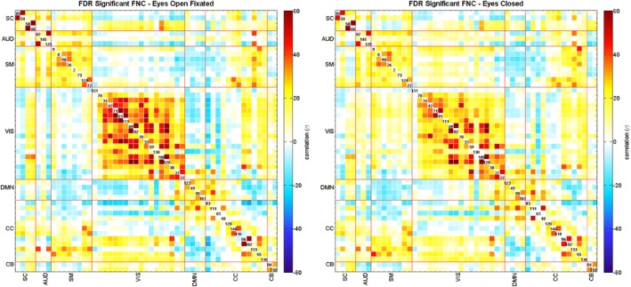
The FNC matrix for all participants, displayed as one sample t‐statistics, thresholded with 0.01 levels FDR. The eyes open––fixated condition is shown on the left and the eyes closed condition is on the right [Color figure can be viewed at http://wileyonlinelibrary.com]

Figure 3.

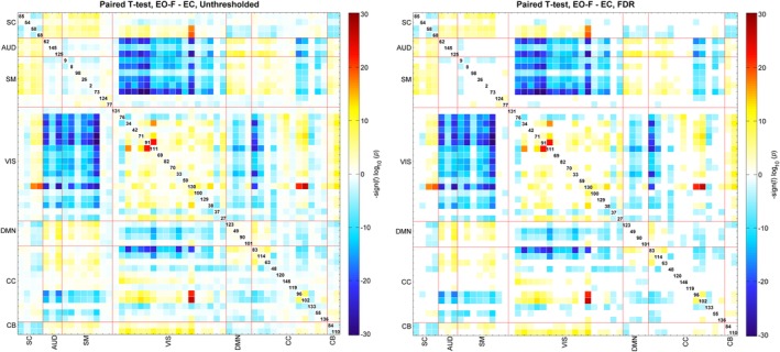
Paired t‐test results for EO‐F and EC FNCs, displayed as −sign(t‐statistics)*log10(p‐value) and on the right 0.01 levels FDR survivors. Blue color shows the regions that have higher correlation in EO‐F case and red color shows the regions that have higher correlation in EC case [Color figure can be viewed at http://wileyonlinelibrary.com]

3.3. Age, gender, and social score effects

We also evaluated the effect of age, gender and social status score on the FNC for EO‐F and EC conditions. We found some FDR‐significant effects for pairs of EO‐F FNC; however, we did not find any FDR‐significant effects for age, gender or social score in the EC condition. The pattern of age effects mostly suggested a decrease in FNC with increasing age in the EO‐F case, and seven pairs of FNC survived multiple comparisons correction. Recall that participants were typically‐developing school age children ranging from 9.1 to 15.5 years old. The pairs surviving multiple comparisons correction were all connectivity of Vis networks and mostly showed a decrease in connectivity with increasing age (Figure 4). FNC between RSN130 (middle occipital gyrus) and networks containing cerebellar regions showed a decrease in connectivity with increasing age; FNC of RSN130 (middle occipital gyrus) with RSN100 and RSN129 (both cerebellar vermis) and RSN84 (right cerebellum). Also FNC between RSN42 (fusiform gyrus and left cerebellum) and RSN100 (cerebellar vermis) also showed a decrease with increasing age. FNC pairs of RSN33 (calcarine gyrus) with RSN38 (left precuneus) and RSN27 (middle cingulate cortex) showed an increase with increasing age. Gender effects were also significant in the EO‐F condition for the FNC pairs of CC network RSN114 (left superior medial frontal gyrus and left temporal pole) with Vis networks, indicating higher correlation in females compared to males (Figure 5). Finally, social status score had a significant effect on FNCs of Cb and Vis networks, suggesting an increase in connectivity with higher social status, and SM networks 26 (right postcentral gyrus) and 2 (left postcentral gyrus) showed a significant decrease in connectivity with increasing social score (Figure 6).

Figure 4.

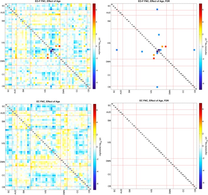
Regression results of the age effect, top figures are for the EO‐F and bottom figures for the EC condition. The results are displayed as −sign(beta)*log10(p‐value). The FDR‐significant results (0.05) are shown to the right. Blue colors show the regions that have lower correlation with increasing age and red colors show the regions that have higher correlation with increasing age [Color figure can be viewed at http://wileyonlinelibrary.com]

Figure 5.

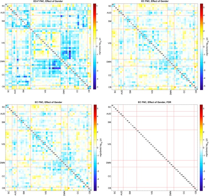
Regression results of the gender effect, top figures are for the EO‐F and bottom figures for the EC condition. The results are displayed as −sign(beta)*log10(p‐value). The FDR‐significant results (0.05) are shown to the right. Blue colors show the regions that have higher correlation in females and red colors show the regions that have higher correlation in males [Color figure can be viewed at http://wileyonlinelibrary.com]

Figure 6.

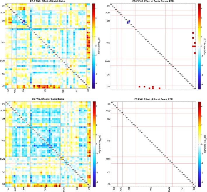
Regression results of the social status score effect, top figures are for the EO‐F and bottom figures for the EC case. The results are displayed as −sign(beta)*log10(p‐value). FDR‐significant results (0.05) are shown to the right. Blue colors show the regions that have lower correlation with increasing social status score and red colors show the regions that have higher correlation with increasing social status score [Color figure can be viewed at http://wileyonlinelibrary.com]

4. DISCUSSION

In this study, we investigated FNC differences using a high ICA model order for resting state EO‐F and EC within a large fMRI dataset. Our results indicated that connectivity within the visual networks showed the most dramatic change between the two different rs‐fMRI conditions, which is intuitive given the vast differences in visual input. The EO‐F condition had significantly more connectivity of Vis networks to themselves and other networks (except for the Aud and SM networks, which had lower connectivity in EO‐F condition), while EC was associated with significantly higher connectivity of Aud and SM networks to other networks. The increase in connectivity of Vis networks is consistent with the interpretation of more organized activation in the visual networks during visual processing, which increases both positive and negative connectivity. The increase in connectivity of SM and Aud networks associated with closing the eyes is consistent with the notion that having closed eyes allows the brain to focus more on other senses like audio and sensation, and thereby increasing connectivity to other networks. This suggests that a similar dynamic change in sensory sensitivity may occur in healthy children and is consistent with the hypothesis of compensation plasticity which states a superior ability in the use of the remaining senses in the early blind population (Liu et al., 2007). However future studies will need to evaluate this more directly.

Our findings are both consistent and inconsistent with previous studies. For instance, Liu et al. (2013) compared FC using seed based analysis with two seeds, left middle occipital gyrus (MOG) and left primary sensory motor cortex (PSMC). They found significantly increased connectivity with the left MOG in the bilateral superior and inferior parietal lobules, widespread regions in the visual cortex, and the right precentral gyrus in EO relative to EC, and found decreased FC with the left MOG mainly within the bilateral PSMC, paracentral lobule, and auditory cortex. These findings were mainly consistent with our results; the Vis network RSN130 in our analysis contains the middle occipital gyrus and it had increased correlation with other Vis network, SC networks and CC networks 96 and 102 (left and right inferior parietal lobule); and showed a significant decrease in FNC with SM and Aud networks during EO‐F relative to EC. On the other hand, Patriat et al. (2013) found that connectivity with a visual seed was significantly modulated by eye condition in a study of 25 participants, which is similar to our results, but they also found greater positive connectivity in the EC case between left visual cortex and higher order visual cortical regions, visual association areas, superior parietal cortex and supramarginal gyrus, while we found greater connectivity in the EO‐F condition. These inconsistent results could be due to the smaller number of participants in the other studies and/or also methodological differences; for example, Patriat et al. (2013) used a seed based analysis.

Another interesting result of our study is that we found significant associations between FNC and age, gender, and social status score only for the EO‐F case. Of note, the association with the EO‐F case was itself limited. This may be due to the fact that the EO‐F represents both a more controlled condition and a condition in which individuals are likely less drowsy. The variability in the EC condition may be greater as a result of participants being in a more drowsy state or to the fact that its less controlled nature may lead to more mind wandering. Of note, Wang, Han, Nguyen, Guo, and Guo (2017) reached higher reliability of FC by removing volumes with high sleepiness, and Patriat et al. (2013); Zou et al. (2015) reported higher test–retest reliability in EO or EO‐F conditions compared to EC. In addition to that, (Allen et al., 2018) reported that according to EEG data; subjects are more likely to get into drowsy/early‐sleep states during EC comparing to EO condition. Future studies should investigate this further and evaluating time‐varying connectivity (Calhoun, Miller, Pearlson, & Adali, 2014) to study these aspects in greater detail.

5. LIMITATION

We should consider some limitations regarding the study. First, we did not have any quantitative metric regarding how well the participant kept their eyes on fixation during the scanning or have a mechanism to check if participant were able to stay awake during the screening. These may introduce some confound to the results. Also, we used an ICA model order of 150, but it would also be interesting to evaluate FNCs differences in EO‐F and EO conditions with higher and lower model orders. Additionally, even though substantial efforts were taken to eliminate confound related to motion and site, residual motion or site related effects could still be present. Finally, we calculated FDR threshold for each covariate separately.

6. CONCLUSION

In conclusion, our study indicated that resting state FNC is significantly affected by the condition (eyes open fixated vs. closed) during scanning. Opening eyes and maintaining fixation was associated with an increase in connectivity of Vis networks to other networks (except from Aud and SM networks which had lower connectivity in EO‐F condition) and themselves, while closing the eyes was linked to a significant increase in connectivity of Aud and SM networks to other networks. Also, we observed EO‐F FNC showed significant association with covariates such as age, gender, and social status scores, but the EC case did not; this could be due to the fact that EO‐F is a more controlled condition that reduces the experimental variability, such as drowsiness, and increases field focus. FNC between Vis and Cb networks increased with higher social status and also FNC between visual areas (middle occipital gyrus) and regions containing cerebellar areas decreased with increasing age. Overall these findings indicated that resting‐state condition has significant effects on the estimated FNC, especially on Vis, Aud, and SM, and suggested that the EO‐F condition may be a better choice for FNC studies that aim to analyze associations with demographic and behavioral covariates.

Agcaoglu O, Wilson TW, Wang Y‐P, Stephen J, Calhoun VD. Resting state connectivity differences in eyes open versus eyes closed conditions. Hum Brain Mapp. 2019;40:2488–2498. 10.1002/hbm.24539

REFERENCES

- Agcaoglu, O. , Miller, R. , Damaraju, E. , Rashid, B. , Bustillo, J. , Cetin, M. S. , … Calhoun, V. D. (2018). Decreased hemispheric connectivity and decreased intra‐ and inter‐ hemisphere asymmetry of resting state functional network connectivity in schizophrenia. Brain Imaging and Behavior, 12(3), 615–630. 10.1007/s11682-017-9718-7 [DOI] [PMC free article] [PubMed] [Google Scholar]
- Agcaoglu, O. , Miller, R. , Mayer, A. R. , Hugdahl, K. , & Calhoun, V. D. (2016). Increased spatial granularity of left brain activation and unique age/gender signatures: A 4D frequency domain approach to cerebral lateralization at rest. Brain Imaging and Behavior, 10(4), 1004–1014. 10.1007/s11682-015-9463-8 [DOI] [PMC free article] [PubMed] [Google Scholar]
- Allen, E. A. , Damaraju, E. , Eichele, T. , Wu, L. , & Calhoun, V. D. (2018). EEG signatures of dynamic functional network connectivity states. Brain Topography, 31(1), 101–116. 10.1007/s10548-017-0546-2 [DOI] [PMC free article] [PubMed] [Google Scholar]
- Allen, E. A. , Damaraju, E. , Plis, S. M. , Erhardt, E. B. , Eichele, T. , & Calhoun, V. D. (2014). Tracking whole‐brain connectivity dynamics in the resting state. Cerebral Cortex, 24(3), 663–676. 10.1093/cercor/bhs352 [DOI] [PMC free article] [PubMed] [Google Scholar]
- Allen, E. A. , Erhardt, E. B. , Damaraju, E. , Gruner, W. , Segall, J. M. , Silva, R. F. , … Calhoun, V. D. (2011). A baseline for the multivariate comparison of resting‐state networks. Frontiers in Systems Neuroscience, 5, 2 10.3389/fnsys.2011.00002 [DOI] [PMC free article] [PubMed] [Google Scholar]
- Bell, A. J. , & Sejnowski, T. J. (1995). An information maximization approach to blind separation and blind Deconvolution. Neural Computation, 7(6), 1129–1159. 10.1162/neco.1995.7.6.1129 [DOI] [PubMed] [Google Scholar]
- Biswal, B. , Yetkin, F. Z. , Haughton, V. M. , & Hyde, J. S. (1995). Functional connectivity in the motor cortex of resting human brain using echo‐planar MRI. Magnetic Resonance in Medicine, 34(4), 537–541. [DOI] [PubMed] [Google Scholar]
- Calhoun, V. D. , & Adali, T. (2012). Multisubject independent component analysis of fMRI: A decade of intrinsic networks, default mode, and neurodiagnostic discovery. IEEE Reviews in Biomedical Engineering, 5, 60–73. 10.1109/RBME.2012.2211076 [DOI] [PMC free article] [PubMed] [Google Scholar]
- Calhoun, V. D. , Adali, T. , Pearlson, G. D. , & Pekar, J. J. (2001). A method for making group inferences from functional MRI data using independent component analysis. Human Brain Mapping, 14(3), 140–151. [DOI] [PMC free article] [PubMed] [Google Scholar]
- Calhoun, V. D. , Miller, R. , Pearlson, G. , & Adali, T. (2014). The chronnectome: Time‐varying connectivity networks as the next frontier in fMRI data discovery. Neuron, 84(2), 262–274. 10.1016/j.neuron.2014.10.015 [DOI] [PMC free article] [PubMed] [Google Scholar]
- Calhoun, Vince , Adali, Tülay , Pearlson, Godfrey , & Pekar T, J. (2002). Group ICA of functional MRI data: Separability, stationarity, and inference. Proceedings of the International Conference on ICA and BSS.
- Cetin, M. , Houck, J. , Rashid, B. , Agcaoglu, O. , Stephen, J. , Sui, J. , … Calhoun, V. (2016). Multimodal classification of schizophrenia patients with MEG and fMRI data using static and dynamic connectivity measures. Frontiers in Neuroscience, 10(466). 10.3389/fnins.2016.00466 [DOI] [PMC free article] [PubMed] [Google Scholar]
- Cordes, D. , Haughton, V. M. , Arfanakis, K. , Carew, J. D. , Turski, P. A. , Moritz, C. H. , … Meyerand, M. E. (2001). Frequencies contributing to functional connectivity in the cerebral cortex in "resting‐state" data. AJNR. American Journal of Neuroradiology, 22(7), 1326–1333. [PMC free article] [PubMed] [Google Scholar]
- Du, Y. , Allen, E. A. , He, H. , Sui, J. , Wu, L. , & Calhoun, V. D. (2016). Artifact removal in the context of group ICA: A comparison of single‐subject and group approaches. Human Brain Mapping, 37(3), 1005–1025. 10.1002/hbm.23086 [DOI] [PMC free article] [PubMed] [Google Scholar]
- Du, Y. , & Fan, Y. (2013). Group information guided ICA for fMRI data analysis. NeuroImage, 69, 157–197. 10.1016/j.neuroimage.2012.11.008 [DOI] [PubMed] [Google Scholar]
- Erhardt, E. B. , Rachakonda, S. , Bedrick, E. J. , Allen, E. A. , Adali, T. , & Calhoun, V. D. (2011). Comparison of multi‐subject ICA methods for analysis of fMRI data. Human Brain Mapping, 32(12), 2075–2095. 10.1002/hbm.21170 [DOI] [PMC free article] [PubMed] [Google Scholar]
- Freire, L. , & Mangin, J. F. (2001). Motion correction algorithms may create spurious brain activations in the absence of subject motion. NeuroImage, 14(3), 709–722. 10.1006/nimg.2001.0869 [DOI] [PubMed] [Google Scholar]
- Friedman, J. , Hastie, T. , & Tibshirani, R. (2008). Sparse inverse covariance estimation with the graphical lasso. Biostatistics, 9(3), 432–441. 10.1093/biostatistics/kxm045 [DOI] [PMC free article] [PubMed] [Google Scholar]
- Haak, K. V. , Marquand, A. F. , & Beckmann, C. F. (2018). Connectopic mapping with resting‐state fMRI. NeuroImage, 170, 83–94. 10.1016/j.neuroimage.2017.06.075 [DOI] [PubMed] [Google Scholar]
- Hart, B. , Cribben, I. , Fiecas, M. , & Alzheimer's Disease Neuroimaging, Initiative . (2018). A longitudinal model for functional connectivity networks using resting‐state fMRI. NeuroImage, 178, 687–701. 10.1016/j.neuroimage.2018.05.071 [DOI] [PubMed] [Google Scholar]
- Himberg, J. , Hyvarinen, A. , & Esposito, F. (2004). Validating the independent components of neuroimaging time series via clustering and visualization. NeuroImage, 22(3), 1214–1222. 10.1016/j.neuroimage.2004.03.027 [DOI] [PubMed] [Google Scholar]
- Liu, D. , Dong, Z. , Zuo, X. , Wang, J. , & Zang, Y. (2013). Eyes‐open/eyes‐closed dataset sharing for reproducibility evaluation of resting state fMRI data analysis methods. Neuroinformatics, 11(4), 469–476. 10.1007/s12021-013-9187-0 [DOI] [PubMed] [Google Scholar]
- Liu, Y. , Yu, C. , Liang, M. , Li, J. , Tian, L. , Zhou, Y. , … Jiang, T. (2007). Whole brain functional connectivity in the early blind. Brain, 130(Pt 8), 2085–2096. 10.1093/brain/awm121 [DOI] [PubMed] [Google Scholar]
- Ma, S. , Correa, N. M. , Li, X. L. , Eichele, T. , Calhoun, V. D. , & Adali, T. (2011). Automatic identification of functional clusters in FMRI data using spatial dependence. IEEE Transactions on Biomedical Engineering, 58(12), 3406–3417. 10.1109/TBME.2011.2167149 [DOI] [PMC free article] [PubMed] [Google Scholar]
- Park, H. J. , Friston, K. J. , Pae, C. , Park, B. , & Razi, A. (2018). Dynamic effective connectivity in resting state fMRI. NeuroImage, 180(Pt B), 594–608. 10.1016/j.neuroimage.2017.11.033 [DOI] [PMC free article] [PubMed] [Google Scholar]
- Patriat, R. , Molloy, E. K. , Meier, T. B. , Kirk, G. R. , Nair, V. A. , Meyerand, M. E. , … Birn, R. M. (2013). The effect of resting condition on resting‐state fMRI reliability and consistency: A comparison between resting with eyes open, closed, and fixated. NeuroImage, 78, 463–473. 10.1016/j.neuroimage.2013.04.013 [DOI] [PMC free article] [PubMed] [Google Scholar]
- Rashid, B. , Blanken, L. M. E. , Muetzel, R. L. , Miller, R. , Damaraju, E. , Arbabshirani, M. R. , … Calhoun, V. (2018). Connectivity dynamics in typical development and its relationship to autistic traits and autism spectrum disorder. Human Brain Mapping, 0(0), 3127–3142. 10.1002/hbm.24064 [DOI] [PMC free article] [PubMed] [Google Scholar]
- Smith, S. M. , Miller, K. L. , Salimi‐Khorshidi, G. , Webster, M. , Beckmann, C. F. , Nichols, T. E. , … Woolrich, M. W. (2011). Network modelling methods for FMRI. NeuroImage, 54(2), 875–891. 10.1016/j.neuroimage.2010.08.063 [DOI] [PubMed] [Google Scholar]
- Smitha, K. A. , Akhil Raja, K. , Arun, K. M. , Rajesh, P. G. , Thomas, B. , Kapilamoorthy, T. R. , & Kesavadas, C. (2017). Resting state fMRI: A review on methods in resting state connectivity analysis and resting state networks. The Neuroradiology Journal, 30(4), 305–317. 10.1177/1971400917697342 [DOI] [PMC free article] [PubMed] [Google Scholar]
- Van Dijk, K. R. A. , Hedden, T. , Venkataraman, A. , Evans, K. C. , Lazar, S. W. , & Buckner, R. L. (2010). Intrinsic functional connectivity as a tool for human connectomics: Theory, properties, and optimization. Journal of Neurophysiology, 103(1), 297–321. 10.1152/jn.00783.2009 [DOI] [PMC free article] [PubMed] [Google Scholar]
- Wang, J. , Han, J. , Nguyen, V. T. , Guo, L. , & Guo, C. C. (2017). Improving the test‐retest reliability of resting state fMRI by removing the impact of sleep. Frontiers in Neuroscience, 11, 249 10.3389/fnins.2017.00249 [DOI] [PMC free article] [PubMed] [Google Scholar]
- Wu, L. , Eichele, T. , & Calhoun, V. D. (2010). Reactivity of hemodynamic responses and functional connectivity to different states of alpha synchrony: A concurrent EEG‐fMRI study. NeuroImage, 52(4), 1252–1260. 10.1016/j.neuroimage.2010.05.053 [DOI] [PMC free article] [PubMed] [Google Scholar]
- Yan, C. , Liu, D. , He, Y. , Zou, Q. , Zhu, C. , Zuo, X. , … Zang, Y. (2009). Spontaneous brain activity in the default mode network is sensitive to different resting‐state conditions with limited cognitive load. PLoS One, 4(5), e5743 10.1371/journal.pone.0005743 [DOI] [PMC free article] [PubMed] [Google Scholar]
- Zou, Q. , Miao, X. , Liu, D. , Wang, D. J. , Zhuo, Y. , & Gao, J. H. (2015). Reliability comparison of spontaneous brain activities between BOLD and CBF contrasts in eyes‐open and eyes‐closed resting states. NeuroImage, 121, 91–105. 10.1016/j.neuroimage.2015.07.044 [DOI] [PubMed] [Google Scholar]