An average sliding window correlation method for dynamic functional connectivity

Abstract

Sliding window correlation (SWC) is utilized in many studies to analyze the temporal characteristics of brain connectivity. However, spurious artifacts have been reported in simulated data using this technique. Several suggestions have been made through the development of the SWC technique. Recently, it has been proposed to utilize a SWC window length of 100 s given that the lowest nominal fMRI frequency is 0.01 Hz. The main pitfall is the loss of temporal resolution due to a large window length. In this work, we propose an average sliding window correlation (ASWC) approach that presents several advantages over the SWC. One advantage is the requirement for a smaller window length. This is important because shorter lengths allow for a more accurate estimation of transient dynamicity of functional connectivity. Another advantage is the behavior of ASWC as a tunable high pass filter. We demonstrate the advantages of ASWC over SWC using simulated signals with configurable functional connectivity dynamics. We present analytical models explaining the behavior of ASWC and SWC for several dynamic connectivity cases. We also include a real data example to demonstrate the application of the new method. In summary, ASWC shows lower artifacts and resolves faster transient connectivity fluctuations, resulting in a lower mean square error than in SWC.

1. INTRODUCTION

Functional magnetic resonance imaging (fMRI) (Friston et al., 1995) allows for a noninvasive way of investigating temporal changes of localized brain activations (Friston et al., 1998; Friston, Holmes, Price, Buchel, & Worsley, 1999). Since its early years, event‐related neural activations have been detected using fMRI in response to varied types of stimuli and task‐based experiments (Friston et al., 1999; Josephs & Henson, 1999). In addition, spontaneous activations occurring while subjects are not engaged in goal‐directed external tasks (also known as resting state) have been consistently observed through the brain (Biswal, Zerrin Yetkin, Haughton, & Hyde, 1995; Cordes et al., 2000). These resting state activations were discovered in localized brain areas forming a consistent set of resting state networks (RSNs) with highly replicable activation patterns (Damoiseaux et al., 2006). One of the first and most widely used methods to study the relationship between RSN activations is temporal correlation which is considered as an assessment of functional connectivity (FC) between two RSNs (Allen et al., 2011; Biswal et al., 1995; Horwitz, 2003; Toro, Fox, & Paus, 2008). These ideas lead to the discovery of FC abnormalities in brain function linked to neuropsychiatric disorders (Calhoun, Maciejewski, Pearlson, & Kiehl, 2008; Greicius, 2008; Woodward & Cascio, 2015).

Many studies make one FC assessment for the whole duration of the fMRI scan assuming a static FC. This view has been challenged by evidence that FC does fluctuate with time even in resting state experiments when no particular external attention is required (Chang & Glover, 2010; Sakoğlu et al., 2010; Sakoglu & Calhoun, 2009a; Sakoglu & Calhoun, 2009b) and that resting state FC changes are related to a succession of mental states occurring within the duration of an fMRI scan (Allen et al., 2014; Chang, Liu, Chen, Liu, & Duyn, 2013). Two major measures can be considered: static functional connectivity (sFC) or dynamic functional connectivity (dFC) that considers the existence of spontaneous fluctuations of FC. One of the main differences among these two FC assessments is the time scale employed. Functional connectivity estimated over a long period of time (generally above 5 min) corresponds to sFC, while a relatively short time window between 30 and 100 s has been proposed as a comparatively good window length for dFC (Wilson et al., 2015). Temporal variation in dFC is commonly obtained by sliding the time window (advancing the position) at a regular interval of typically one step, which has been used in other fields previously (Schulz & Huston, 2002), a procedure commonly known as sliding window correlation (SWC). Other window‐based methods of dFC estimation have been developed; however, there is evidence that their performance is similar to SWC for typical window lengths (larger than 30 s) (Xie et al., 2018). SWC has become a common technique to assess dFC (Hutchison et al., 2013; Sakoğlu et al., 2010; Shakil, Lee, & Keilholz, 2016), offering both easy implementation and easy interpretation. In the current state of the art, window length selection remains one of the most discussed topics and further development is necessary to determine the best choice for this parameter (Preti, Bolton, & Van De Ville, 2017).

In spite of evidence for the existence of temporal FC fluctuations, an important concern in the field is to identify whether estimated dFC is effectively due to real changes of FC or corresponds to a static signal corrupted by unrelated nuisances and artifacts. The relatively short temporal span of SWC makes it particularly sensitive to nuisances such as scanner drift, head motion, and physiological noise (Hutchison et al., 2013). Statistical tests for the detection of dynamicity in estimated time series of FC have been proposed based on different factors such as variance (Hindriks et al., 2016; Sakoğlu et al., 2010), Fourier‐transformed time‐series (Handwerker, Roopchansingh, Gonzalez‐Castillo, & Bandettini, 2012) and nonlinear statistics (Zalesky, Fornito, Cocchi, Gollo, & Breakspear, 2014). Most statistical procedures look to test the null hypothesis H₀ that FC does not change with time. Once H₀ has been rejected, the next important step is to reduce variability due to random noise and nuisances without compromising the estimation of the true dFC.

In addition to scanner drift, head motion, and physiological noise (Hutchison et al., 2013), SWC outcomes can be affected by the selection of the window length parameter (Sakoğlu et al., 2010; Shakil et al., 2016). Window length is expected to be large enough to allow for a robust estimation of the correlation coefficient, but also small enough to detect transient variations (Hutchison et al., 2013; Sakoğlu et al., 2010). Some studies warn about the existence of spurious fluctuations in the SWC method proposing a rule of thumb to reduce these nuisances that sets the SWC window length to 1/f₀ s or larger, where f₀ corresponds to the smaller frequency in the spectrum (Leonardi & Van De Ville, 2015; Zalesky & Breakspear, 2015). The spectrum of interest for fMRI has been proposed to start at 0.01 Hz after studying frequencies dominated by neuronal activity and away from physiological noise such as cardiac and respiratory activity (Chen & Glover, 2015; Fransson, 2005). At the higher end, it has been found that neuronal information is concentrated in the range below 0.10 Hz (Cordes et al., 2001), but evidence suggests that important contributions of lower amplitude exist for frequencies above 0.10 Hz (Chen & Glover, 2015). Because of the rule of thumb 1/f₀, it has been suggested that dFC will suffer from spurious artifacts unrelated to the true signal if the window length is chosen below 100 s (Leonardi & Van De Ville, 2015). Although choosing larger window lengths is an option, time scales well beyond a minute (i.e., including the 100 s mark) may suppress frequency content that characterizes dFC (Zalesky & Breakspear, 2015). Instead of a large time scale, this work proposes to perform an average SWC (ASWC) seeking a better dFC estimation and reducing the window length. In general, averaging repeated measures of correlation coefficients is a way of increasing the accuracy of estimated correlation (Corey, Dunlap, & Burke, 1998; Silver & Dunlap, 1987). This idea derives from the basic statistical principle that the standard error of the average decreases as the number of observations increases. The proposed procedure is to average a predefined number of consecutive SWCs and then advance one step and average the next set of SWCs. Through theoretical mathematical characterization and simulation experiments, we demonstrate that ASWC time scales of about 94 s (windowing plus averaging) are enough to reduce spurious artifacts and account for the 0.01 Hz frequency cut‐off. Optimal SWC and ASWC configurations are compared and the effect of reduced sensitivity to dFC variations is demonstrated through simulations.

2. ANALYSIS OF AVERAGE SLIDING WINDOW CORRELATION

2.1. Background

Leonardi and Van De Ville (Leonardi & Van De Ville, 2015) proposed an approximate model to warn about the presence of artifacts in the SWC approach. Their theoretical development utilizes properly normalized cosines $x\left[k\right]=\sqrt{2}\cos \left(\mathit{\text{ωkTR}}\right)$ and $y\left[k\right]=\sqrt{2}\cos \left(\mathit{\text{ωkTR}}+\theta \right)$ of angular frequency ω = 2πf (where the frequency f is measured in Hertz) and a phase difference of θ. The two cosines are evaluated at time points kTR where the constant TR is specific to the fMRI scanning protocol and k ∈ {0, 1, 2, …}. The purpose of factor $\sqrt{2}$ is to normalize variances C_xx and C_yy to one. Under the condition that C_xx = C_yy = 1, it follows that covariance equals correlation ${\rho }_{\mathit{xy}}=C_{\mathit{xy}}/\sqrt{C_{\mathit{xx}}{C}_{\mathit{yy}}}=C_{\mathit{xy}}$. Furthermore, the phase difference θ is related to correlation by ρ_xy = cos(θ) if the correlation is calculated over a window length 1/f (i.e., over a period of the cosines). To study the effects caused by other windowing conditions, we define the SWC length as h = 2ΔTR where Δ ∈ {1, 2, …} is a predefined number of time points. For a more detailed explanation of the setting h = 2ΔTR see the Supporting Information Appendix S1 Part 1. Defining $\overline{x}\left[n\right]$ and $\overline{y}\left[n\right]$ as the cosine averages at point n over the interval [(n − Δ)TR, (n + Δ)TR], the covariance at each point n can be written as

$$C_{\mathit{xy}}\left[n\right]=\frac{\mathit{TR}}{h}\sum _{k=n-\Delta +1}^{n+\Delta }x\left[k\right]y\left[k\right]-\overline{x}\left[n\right]\overline{y}\left[n\right].$$ (1)

A closed‐form equation for the covariance term was then obtained after approximating the sum using integrals (see Supporting Information Appendix S1 Part 3) resulting in (Leonardi & Van De Ville, 2015)

$$C_{\mathit{xy}}\left[n\right]=\cos \left(\theta \right)+\frac{1}{\mathit{h\omega }}\cos \left(2\mathit{\text{ωnTR}}+\theta \right)\sin \left(2\omega \Delta \mathit{TR}\right)-\frac{8}{h^2{\omega }^2}\cos \left(\mathit{\text{ωnTR}}\right)\cos \left(\mathit{\text{ωnTR}}+\theta \right){\sin }^2\left(\omega \Delta \mathit{TR}\right).$$ (2)

Simulation results of this model are summarized in Figure 1. Figure 1a shows two properly normalized cosines used for further simulation. Figure 1b displays the outcome of varying the SWC length h and sliding the window at different time points nTR replicating the same simulation experiments found through the literature (Leonardi & Van De Ville, 2015; Zalesky & Breakspear, 2015). As the SWC length h increases the terms at the right of cos(θ) in (2) vanish and the covariance approaches the correlation. The suggestion of limiting h to 1/f_min can be understood by recognizing that artifacts have their largest dynamic range in the interval 0 < h < 1/f (between 0 and 40 s in Figure 1b). Notice that larger window lengths (i.e., 1/f < h) result in smaller artifact fluctuations. Also notice that, in spite of artifact reduction, the observed nuisance fluctuations are not guaranteed to disappear for 1/f < h. This fact is demonstrated by the second artifact lobe, occurring at h = 48 s in Figure 1b. In this work, we propose the use of ASWC to further reduce artifacts. Averaging has been performed in Figure 1c for the second lobe of artifacts in Figure 1b (h = 48 s), briefly illustrating how artifacts can be reduced through ASWC. In the following sections, we will make a theoretical characterization of the artifact reduction shown in Figure 1c to better explain the effects of ASWC.

Figure 1.

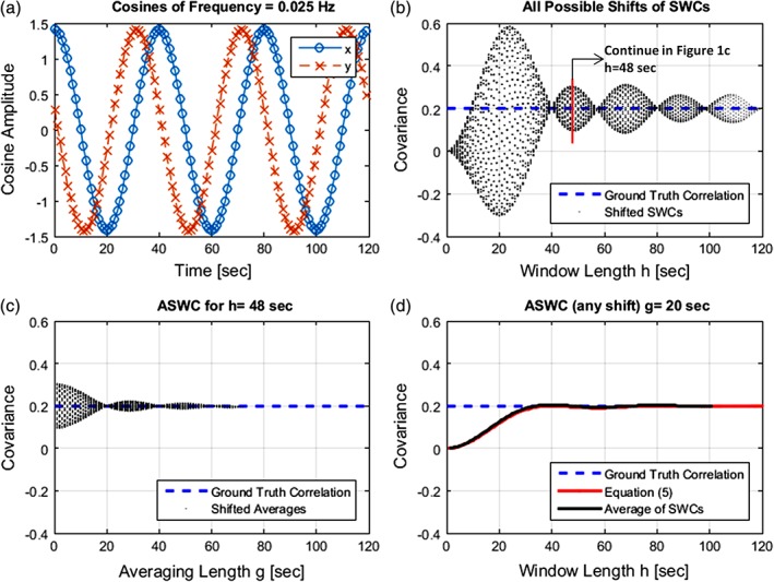
Averaging of the cosine model for a simulated correlation of 0.2. (a) The two cosines at the upper left plot were generated assuming a TR = 1 s, a frequency of f = 0.025 Hz and a phase difference given by θ = arccos(0.2). (b) Sliding window correlations (SWCs) were estimated at all possible shifts of one TR and for SWC lengths from 2 to 120 s. For a given window length, the SWC value depends on the time shift. SWCs for all time shifts are plotted on the upper right figure using small black dots. In this example, following the recommended SWC length (Leonardi & Van De Ville, 2015) will result in f_min = 0.025 Hz and h_min ≥ 1/f_min = 40 s. However, this figure shows that artifacts are still strong around approximately h = {50, 70, ⋯}. (c) The bottom left plot shows the effect of averaging for the window length h = 48 s, point where the stronger artifacts occur for that lobe. Spurious variability of SWCs disappears at the averaging length g =1/2f = 20 s. (d) the bottom right plot shows the resulting SWC value (black line) as a function of h at averaging length g = 20 s. The SWC values are independent of the time shift selected. For comparison, the asymptotic averaging result g → ∞ obtained in quation 5 is displayed in red. The two average settings g = 1/2f and g → ∞ lead to the same result [Color figure can be viewed at http://wileyonlinelibrary.com]

2.2. Mathematical characterization of ASWC

As displayed in Figure 1, mismatches between window length h and frequency f introduce spurious fluctuations unless tuning h = 1/f is achieved. This tuning is obtained from setting ωΔTR = π and solving for h = 2ΔTR, which complies with the rule of thumb h ≥ 1/f (Leonardi & Van De Ville, 2015) and sets the two sine functions in (2) to zero. As the frequency spectrum of real data is generally not composed of a singleton frequency, imperfect tuning is likely to exist along with spurious fluctuations from untuned frequencies. Given that spurious fluctuation artifacts might be unavoidable, the next option is to minimize the impact of artifacts. One possibility to address the lack of tuning is to consider large window lengths given the factor 1/h in (2), which predicts improved estimation accuracy as h increases. This procedure is not convenient as larger window lengths decrease the sensitivity of detecting transient fluctuations of FC (Hutchison et al., 2013). Instead of increasing h as a method of decreasing artifacts, we consider the option of taking g consecutive SWCs and averaging them to improve the estimation of correlation. To mathematically characterize ASWC, we define the averaging interval g = 2∇TR from m − ∇ to m + ∇ (where ∇ is a parameter used to select the averaging length) and perform a similar integral approximation as that proposed in (Leonardi & Van De Ville, 2015). We thus define the average correlation ${\overline{C}}_{\mathit{xy}}\left[m\right]$ at a time point defined by m over the averaging interval [(m − ∇)TR, (m + ∇)TR] as

$${\overline{C}}_{\mathit{xy}}\left[m\right]=\frac{\mathit{TR}}{g}\sum _{m-\nabla +1}^{m+\nabla }{C}_{\mathit{xy}}\left[m\right]\approx \frac{1}{g}\underset{\left(m-\nabla \right)\mathit{TR}}{\overset{\left(m+\nabla \right)\mathit{TR}}{\int }}{C}_{\mathit{xy}}\left(t\right)\mathit{dt}.$$ (3)

After performing the integral (3) described in the Supporting Information Appendix S1 Part 4, the averaging equation can then be written as

$${\overline{C}}_{\mathit{xy}}\left[m\right]=\cos \left(\theta \right)\mathrm{K}\left(h,\omega ,\mathit{TR}\right)+\cos \left(2\mathit{\text{ωmTR}}+\theta \right)\mathrm{\Psi }\left(g,h,\omega ,\mathit{TR}\right)$$ (4)

where

$$\mathrm{K}\left(h,\omega ,\mathit{TR}\right)=\left(1-\frac{4}{h^2{\omega }^2}{\sin }^2\left(\omega \Delta \mathit{TR}\right)\right)$$

and

$$\mathrm{\Psi }\left(g,h,\omega ,\mathit{TR}\right)=\frac{2}{\mathit{gh}{\omega }^2}\sin \left(2\omega \nabla \mathit{TR}\right)\sin \left(\omega \Delta \mathit{TR}\right)\left[\cos \left(\omega \Delta \mathit{TR}\right)-\frac{2}{\mathit{h\omega }}\sin \left(\omega \Delta \mathit{TR}\right)\right].$$

The first term cos(θ)K(h, ω, TR) of (4) describes the effects that are independent of averaging length g and averaging position m since none of the factors cos(θ) and K(h, ω, TR) include g or m. On the other hand, the second term of (4) cos(2ωmTR + θ)Ψ(g, h, ω, TR) describes sinusoidal type artifacts containing a frequency 2ω twice higher than that of the original signal. This term can be zeroed by setting it at sin(2ω ∇ TR) = 0, which results in Ψ(g, h, ω, TR) = 0. This condition can be met if 2ω ∇ TR = kπ where k ∈ {…, −2, −1, 0, 1, 2, …}. As g = 2 ∇ TR and ω = 2πf, solving 2ω ∇ TR = kπ for g results in g = k/(2f). Figure 1c shows an averaging simulation where the different points of sin(2ω ∇ TR) = 0 can be observed. This means for example that if f= 0.025 Hz the specific averaging length is g = 1/(2 * 0.025) s = 20 s to zero the second term in (4). Although a similar analysis could be applied to h by forcing sin(ωΔTR) = 0 in (4), setting h = 1/f causes estimation inaccuracies due to effects described by K(h, ω, TR) that will be explained in the next section. In addition, Figure 1d illustrates how all estimation variability is eliminated once g = k/(2f), including artifacts in the range h ≥ 1/f. Notice that Figure 1d replicates the simulation experiment from Figure 1b, but includes an averaging step of length g = 1/(2f)= 20 s, zeroing all artifacts for h ≥ 1/f. As we have set Ψ(g, h, ω, TR) = 0 in Figure 1d, the observed behavior corresponds to K(h, ω, TR) where the estimation inaccuracy follows a monotonic trend in the range h ≤ 1/f.

Equations developed in this section predict a series of advantageous effects after averaging. The SWC artifact fluctuations due to lack of the tuning h = 1/f (illustrated in Figure 1b) can be completely obliterated by the implementation of the ASWC method with appropriate tuning g = 1/(2f) as predicted by (4) and simulated in Figure 1d. While it is true that real data are characterized by complex frequency spectrums that do not allow for complete artifacts elimination, there is an important reduction of artifacts even for nonmatching averaging lengths. This reduction is illustrated in Figure 1c where a wide range of averaging lengths were tested, showing that artifacts are the strongest for the no averaging case (g=0). The equations we present show that ASWC have weaker artifacts than SWC because of two important factors. First, the strongest SWC artifacts diminish at a rate of 1/h as shown in the second term of (2). In contrast, it is predicted by (4) that artifact reduction in ASWC is stronger through a quadratic factor 1/h² and a factor with combined window and averaging lengths 1/gh. Second, in both SWC and ASWC it is expected that artifact fluctuations diminish as the frequency increases. However, ASWC artifacts decrease quadratically through the factor 1/ω² (ω = 2πf) compared with the SWC artifacts with a slope that depends on 1/ω. Equations also predict an ASWC with advantages over SWC even for non‐ideal matching between configured parameters and frequency. It is evident at this point that studying the effects of frequency is an important next step in this development since real signals likely contain complex frequency content.

2.3. Asymptotic analysis of artifacts and frequency

Our discussion will now move away from the averaging artifact term Ψ(g, h, ω, TR) discussed in the previous subsection and focus on the term K(h, ω, TR) that has a strong dependence with frequency. As previously explained, factor Ψ(g, h, ω, TR) can be zeroed out by tuning the averaging length, but also by taking the asymptote g → ∞. For the current presentation, we introduce the use of the function sinc(x) = sin(πx)/πx to simplify K(h, ω, TR) as K(h, f, TR) = (1 − sinc²(fh)). The derivation of this equation can be found in the Supporting Information Appendix S1 Part 5. When the averaging length approaches the values of interest g → ∞ and g → 1/(2f) leading to Ψ(g, h, ω, TR) = 0, this produces the frequency dependent limit

$$\underset{\begin{array}{c}g\to \infty \\ \mathit{\text{or}}\\ g\to 1/\left(2f\right)\end{array}}{\lim }{\overline{C}}_{\mathit{xy}}\left[m\right]=\cos \left(\theta \right)\left(1-{\mathrm{sinc}}^2\left(\mathit{fh}\right)\right).$$ (5)

For the purpose of simplifying the exposition, we will call (5) the asymptotic behavior of (4). Notice that the results from averaging over a long time scale (i.e., g → ∞) are more compatible with real data than tuning g → 1/(2f). For the moment, we assume that either asymptote will be achieved and ${\overline{C}}_{\mathit{xy}}\left[m\right]$ can be described by cos(θ)(1 − sinc²(fh)). Mathematically, the function is an inverted sinc²(x) where the highest variability occurs at its main lobe with some small side lobes for values x > 1. Figure 2a displays the inverted lobe behavior of (1 − sinc²(x)) for the product x = fh. Notice that achieving (1 − sinc²(fh)) = 1 in (5) allows for a perfect estimation. In this case, deviations from (1 − sinc²(fh)) = 1 describe the estimation error. These deviations from 1 occur because of the side lobes of (1 − sinc²(fh)) that weaken as the product fh increases. The maximum error occurs at the first side lobe (see Figure 2a) where (1 − sinc²(fh)) = 0.9528 (an error of 1 − (1 − sinc²(fh)) = 0.0472) representing the largest estimation error according to (5) for the range fh ≥ 1. Under the studied conditions, this estimation error is less than a 5% error. The effect of this asymptotic behavior for different values of f and h is illustrated in Figure 2b where the neighborhood of fh = 1 (the first wide white band after the dark red area in Figure 2b) results in an exact estimation while some small vanishing lobes (less than 5% error as discussed) are observed for fh > 1.

Figure 2.

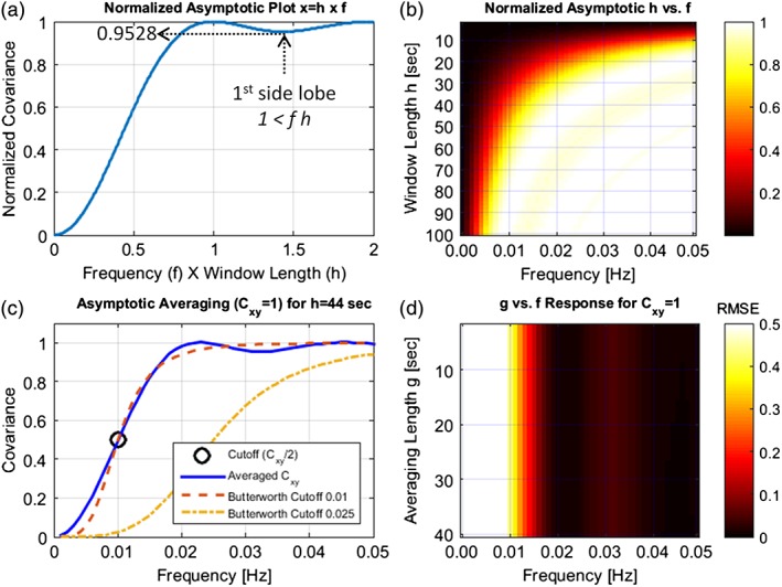
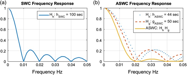
Asymptotic response of ASWCs. (a) The left top plot displays the shape of asymptote (5) described by (1 − sinc²(x)) for the factor x = fh, where f is the frequency and h is the window length. (b) The right top plot illustrates the deleterious effects (perfect covariance estimation (${\overline{C}}_{\mathit{xy}}=1$) is indicated by white areas) predicted by (5) on covariance estimation for a range of values of f and h. This result indicates that low frequencies and low window lengths (dark red areas) must be avoided as they result in the largest deviation from ground truth. (c) The bottom left panel features a 15 min simulation using two identical cosines with ${\overline{C}}_{\mathit{xy}}=1$ for the same window length of 44 s but varying frequency. Since h = 44 s the cutoff frequency estimated by (6) is 0.01 Hz which is indicated by the circle drawn in the plot. The plot also shows how the filter compares to second order Butterworth filters using cutoffs of 0.01 Hz and 0.025 Hz. (d) The bottom right plot shows the root mean square error (RMSE) (averaged over 15 min) after setting h = 44 s for different frequencies and averaging lengths. The largest observed RMSE was 1.27, but fitting the color range to this value left obscured other smaller errors; hence, this plot was instead scaled to the (0, 0.5) range. The figure clearly shows the cut‐off 0.5 at 0.01 Hz, an observation that does not change with the averaging length [Color figure can be viewed at http://wileyonlinelibrary.com]

The next step in our analysis focuses on the interplay between frequency ω = 2πf and window length h. As a first sanity check, let h → ∞ or ω → ∞ to see that K(h, ω, TR) approaches 1; that is a perfect asymptotic estimation according to (5). For the other direction h → 0 or ω → 0, Figure 2a illustrates how small values of h or ω fall within the main inverted lobe with a behavior given by the limit $\underset{h\to 0}{\lim }\mathrm{K}\left(h,\omega ,\mathit{TR}\right)=\underset{\omega \to 0}{\lim }\mathrm{K}\left(h,\omega ,\mathit{TR}\right)=0$. Thus, the power for low frequencies is reduced all the way down to zero similar to a high pass filter. The point of perfect estimation is defined by sinc²(fh) = 0, or fh = 1 → h = 1/f, providing a second sanity check point. Notice that all described conditions h = 1/f, h → ∞ and ω → ∞ agree with the SWC features previously predicted for SWC; see (2) and (Leonardi & Van De Ville, 2015). In contrast to SWC, the ASWC equations predict a high pass filter behavior. In the next section, we theoretically demonstrate that the resulting ASWC filter can be tuned to remove low frequency content, allowing the removal of frequencies below 0.01 Hz.

2.4. ASWC filtering

Here, we refocus our attention on the analysis of the ASWC/SWC problem from the frequency perspective. The approximation in (5) allows tracking the magnitude of covariance for a singleton frequency given that the sliding window length h is constant. This assumption is more relevant in practice since the window length is commonly chosen and left unchanged through the analysis of real data (Allen et al., 2014). For the moment, we will continue assuming the asymptotic behavior (5), where ${\overline{C}}_{\mathit{xy}}\left[m\right]=\cos \left(\theta \right)\left(1-{\mathrm{sinc}}^2\left(\mathit{fh}\right)\right)$. Setting h constant leaves frequency f as the only variable of interest. Figure 2c illustrates how Equation 5 describes a high pass filter type relationship between averaged covariance and frequency with an approximate product hf₀ (where f₀ is the cut‐off frequency)

$$h{f}_0\approx \sqrt{\frac{10}{{\pi }^2}\left(1-\sqrt{1-\frac{6}{5}\left(1-\sqrt{1-\mathrm{\alpha }}\right)}\right)}\approx {\left.0.4441\right|}_{\alpha =1/2}.$$ (6)

The approximation (6) can be obtained using the Taylor expansion of sinc(x) ≈ 1 − π²x²/6 + π⁴x⁴/120 and its derivation is displayed in the Supporting Information Appendix S1 Part 6. We present the whole approximation for the general case where a covariance threshold ${\overline{C}}_{\mathit{th}}$ ($\alpha ={\overline{C}}_{\mathit{th}}/{\overline{C}}_{\mathit{max}}$) is required. For the purposes of filter design, the cut‐off frequency is the point where the filter cuts frequency power in half; thus the value ${\alpha }_{\mathit{cut}-\mathit{off}}={\overline{C}}_{\mathit{th}}/{\overline{C}}_{\mathit{max}}=1/2$. Equation 6 was evaluated for α = 1/2 to provide a simple way of tuning the ASWC window length to the required frequency response.

2.5. Comparing tuned SWC and tuned ASWC

In wide band signals, both techniques SWC and ASWC will suffer from spurious fluctuations due to the existence of non‐tuned frequencies. The important concern we must answer next is, if there are values satisfying the inequality g_ASWC + h_ASWC < h_SWC with reduced power of unavoidable artifact fluctuations. We did this comparison using a simulation spanning frequencies from 0 to 0.10 Hz. Before estimating the SWC, we applied a typical high pass fifth‐order Butterworth filter but did not use the filter for the ASWC. With this procedure, we are using the natural filtering characteristics of ASWC shown in Figure 2c. The Butterworth filter order in the SWC simulation is the same as that previously recommended (Allen et al., 2011). As we are interested in a cut‐off frequency of f₀= 0.01 Hz, we set h_SWC = 1/f₀. Following the recommendation in Equation 6, we set h_ASWC = 0.4441/f₀≈ 44 s. The frequency response for h_ASWC= 44 s is illustrated in Figure 2c As illustrated in Figure 1, the averaging length should be g_ASWC = 1/(2f₀) and adjusting to the current frequency of interest (i.e., 0.01 Hz) gives g_ASWC=50 s. Notice that selected values comply with the inequality g_ASWC + h_ASWC < h_SWC. Figure 3 displays the simulation outcomes where h_SWC= 100 s, h_ASWC= 44 s and g_ASWC= 50 s. According to Equation 6, larger window lengths decrease the ASWC cut‐off, but we need to keep low frequencies of no interest controlled by fixing the cut‐off at 0.01 Hz. Shorter window lengths will move the ASWC cut‐off above 0.01 Hz, thus removing important frequency content. We compared the power of artifact fluctuations by estimating their standard deviations σ_SWC and σ_ASWC for each corresponding method. Figure 3c displays the ratio σ_SWC/σ_ASWC for each frequency. The plots for SWC and ASWC show similar trends for low frequencies, but this trend is in part related to the fifth‐order filter. The frequency cut‐off in ASWC can be clearly observed in Figure 3b at 0.01 Hz, where the predicted covariance is 0.5. At higher frequencies, the fluctuations in ASWC look smaller compared to those from the SWC. The plot for σ_SWC/σ_ASWC in Figure 3c further confirms this observation. Starting from the cut‐off 0.01 Hz, we can see that ASWC has a clear advantage over SWC. At higher frequencies, the ratio σ_SWC/σ_ASWC peaks close to 2¹⁰ and indicates that the standard deviation of SWC fluctuations could be as high as 1,024 times larger than fluctuations in ASWC.

Figure 3.

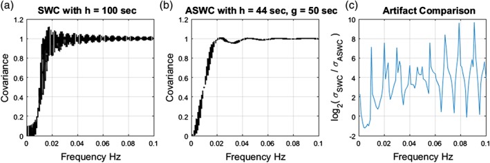
Comparing larger SWC length versus averaging using the same number of samples. The simulation in this plot was performed with a TR = 1 s and estimations were taken over 5 min. In the first panel (a), a window length of h_SWC= 100 s was selected and the result was not averaged. A fifth‐order high pass Butterworth filter with cut‐off 0.01 Hz was applied to remove low frequencies of no interest. We can see the existence of spurious SWCs at frequencies not tuned to 1/100 Hz. In panel (b), time points were redistributed to have a window length of h_ASWC= 44 s and an averaging length of g_ASWC= 50 s. No filter was applied; the simulation used the natural filtering of ASWC described in Figure 2c, a tuned fit the 0.01 Hz cut‐off. (c) The ratio of standard deviations σ_SWC/σ_ASWC has been plot in a logarithmic scale showing that SWC exhibit higher artifact power than ASWC at frequencies higher than the cut‐off 0.01 Hz [Color figure can be viewed at http://wileyonlinelibrary.com]

2.6. Sharp phase transitions

Sliding windows are used in the context of dynamic changes of coherence, but equations so far have been applied to a static constant phase. This is not practical as the focus of dynamic connectivity is to study the temporal changes of correlation ρ_xy. Correlation dynamics can be characterized in the single frequency covariance model by temporal variations of the cosine phase θ. The following analysis presents a theoretical development based on the simple and tractable case of a sharp cosine phase transition and also generalizes to describe a more practical situation.

The next stage is to mathematically characterize phase transitions. The simplest of these transitions is a sharp change at a given time point t₀ = 0. Before t₀, let the two cosines x[k] and y[k] have phases γ and θ respectively, and after t₀, let the phases update to φ and φ. We first reformulate the SWC analysis from (2) in a way that includes the four phases (γ, θ, φ, and ϕ), resulting in

$$\begin{array}{c}{C}_{\mathit{xy}}\left[n\right]=\frac{\mathit{TR}}{h}\sum _{k=n-\Delta +1}^{n+\Delta }x\left[k\right]y\left[k\right]\approx \frac{2}{h}\left[\underset{\left(n-\mathrm{\Delta }\right)\mathit{TR}}{\overset{0}{\int }}\cos \left(\mathit{\omega t}+\gamma \right)\cos \left(\mathit{\omega t}+\theta \right)\mathit{dt}+\underset{0}{\overset{\left(n+\mathrm{\Delta }\right)\mathit{TR}}{\int }}\cos \left(\mathit{\omega t}+\phi \right)\cos \left(\mathit{\omega t}+\varphi \right)\mathit{dt}\right]\\ =\frac{\left(\mathrm{\Delta }-n\right)\mathit{TR}}{h}\cos \left|\gamma -\theta \right|+\frac{\left(\mathrm{\Delta }+n\right)\mathit{TR}}{h}\cos \left|\phi -\varphi \right|+\frac{1}{h}\left[\underset{\left(n-\mathrm{\Delta }\right)\mathit{TR}}{\overset{0}{\int }}\cos \left(2\mathit{\omega t}+\gamma +\theta \right)\mathit{dt}+\underset{0}{\overset{\left(n+\mathrm{\Delta }\right)\mathit{TR}}{\int }}\cos \left(2\mathit{\omega t}+\phi +\varphi \right)\mathrm{d}t\right].\end{array}$$

 

To go from the first line to the second, we used the identity $\cos \left(a+b\right)\cos \left(a+c\right)=\frac{1}{2}\left(\cos \left|b-c\right|+\cos \left(2a+b+c\right)\right)$. The covariance then approximates a weighted sum of the cosines of phase differences plus a term ℶ_h that depends on 1/h. The covariance term can be expressed as

$$C_{\mathit{xy}}\left[n\right]=\frac{\left(\mathrm{\Delta }-n\right)\mathit{TR}}{h}\cos \left|\gamma -\theta \right|+\frac{\left(\mathrm{\Delta }+n\right)\mathit{TR}}{h}\cos \left|\phi -\varphi \right|+{\mathrm{\beth }}_h.$$ (7)

The next step is to average (7) to obtain the ASWC equation. Due to their linearity, averaging the weighted sum $\frac{\left(\mathrm{\Delta }-n\right)\mathit{TR}}{h}\cos \left|\gamma -\theta \right|+\frac{\left(\mathrm{\Delta }+n\right)\mathit{TR}}{h}\cos \left|\phi -\varphi \right|$ does not change the sum. For a more formal analysis see the Supporting Information Appendix S1 Part 7. On the other hand, the artifacts term ℶ_h changes and the averaged result ${\overline{\beth }}_{h,g}$ depends on the window length h and the averaging length g. The ASWC version of the sharp phase transition model is then

$${\overline{C}}_{\mathit{xy}}\left[m\right]=\frac{\left(\mathrm{\Delta }-m\right)\mathit{TR}}{h}\cos \left|\gamma -\theta \right|+\frac{\left(\mathrm{\Delta }+m\right)\mathit{TR}}{h}\cos \left|\phi -\varphi \right|+{\overline{\mathrm{\beth }}}_{h,g}.$$ (8)

Simulations of the sharp phase transition model are presented in Figure 4. In this figure and the other figures ahead in this work, we followed the convention that covariance estimates are positioned in the middle of the computation range. For example, the range in an SWC is [(n − Δ)TR, (n + Δ)TR] and covariance C_xy[n] is defined at the time point nTR. Thus, the first time point suitable for a complete SWC simulation starts at ΔTR. At the other end, simulations stop at ΔTR seconds before the last sample of the sinusoidal time course. In the case of ASWC, the total range of correlation plus averaging is [(m − (∇ + Δ))TR, (m + (∇ + Δ))TR] and the time shifts that apply at both ends of the simulation are defined by (∇ + Δ)TR. Figure 4b displays a simulation result where the influence of the SWC term ℶ_h is evident from the observed spurious fluctuations. However, averaging reduces the spurious artifacts as shown in Figure 4b Simulation results thus suggest that ${\overline{\beth }}_{h,g}$ characterizes weaker artifacts as those described by ℶ_h. In addition, the artifact term ${\overline{\beth }}_{h,g}$ depends on both 1/h and 1/g, hence generally exhibiting a weaker strength than ℶ_h that only depends on 1/h.

Figure 4.

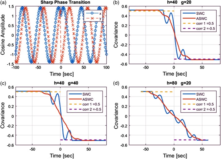
This plot shows a sharp correlation transition from 0.5 to − 0.5. (a) The two cosines (f = 0.025 Hz) suffer a phase change at time t = 0 defining four different phases distributed among the two cosines. The phases were selected to simulate the configured correlations: Cosine in blue shifted phase from π/4 to −π/4 radians, the red cosine from (π/4 − 0.5) to (−π/4 + 0.5) radians. (b) Performing a tuned SWC with h = 40 s shows the effect of the phase transition resulting in sinusoidal‐like artifacts. The effect of averaging with g = 1/2f = 20 s reduces the artifacts, but neither the phase transition nor the weighted averaging trend are removed as predicted in (7) and (8). (c) In this plot we doubled the averaging length (g = 40 s) resulting in little change with respect to the original setup. (d) Larger differences are observed when doubling the window length (h = 80 s). As predicted in (8), changes in the window length will have a larger effect than changes in the averaging length [Color figure can be viewed at http://wileyonlinelibrary.com]

Although the closed form of the artifact terms ℶ_h and ${\overline{\beth }}_{h,g}$ were not developed due to their complexity, we can expect that averaging reduces artifacts following a similar behavior as that described in (2) and (4). We will call the first two terms in (7) and (8) the estimation terms since they allow tracking the covariance variation of the sharp phase transition. Figure 4 displays a sharp phase transition simulation for SWC and ASWC versions of the covariance estimation and assume a perfect tuning for two intervals where correlation is constant. As in the static case of (2) and (4), averaging in Figure 4b decreased the artifact fluctuations present in SWC. The most important result from (8) is that averaging does not change the estimation terms of the sharp edge Equation 8. Thus, the averaging length does not affect the estimation terms and only decreases the strength of the artifact term ${\overline{\beth }}_{h,g}$. This is illustrated by Figure 4b,c where there are small changes in fluctuation but not in the overall estimation when averaging length is doubled. On the contrary, the window length has a key role in defining the weights within the estimation terms. Thus, the window length has a large influence on the estimation. Figure 4d illustrates the loss of estimation sharpness due to doubling the window length. These results indicate that it is more important to reduce the window length h than reduce the averaging length g as h has a greater influence in the estimation.

2.7. A moving average model (beyond sharp phase transitions)

Figure 4 shows the complete obliteration of ASWC sinusoidal artifacts as predicted by (4) for properly tuned window and averaging lengths. The sharp edge transition explains how the selection of a window length can have a large impact in resolving transient changes in phase. Despite predicting artifact reduction after averaging, the sharp phase transition model is limited to one phase transition between two constant phase intervals. Nonetheless, the trend of reduced artifacts can be expected to be similar for more complex configurations. For example, two sharp transitions will eventually be characterized as the weighted sum of the three different phases plus the artifact term, which in our case will depend on the choice of SWC or ASWC. Furthermore, increasing the number of sharp transitions can characterize increasingly smooth changes of phase and correlation through time. After considering a sufficiently large number of transitions, SWC can be described by the weighted average over a large number of time intervals, each with a weight w_k, and a given phase difference θ_k plus an artifact term such that

$$C_{\mathit{xy}}\left[n\right]=\left(\sum _k{w}_k\cos \left({\theta }_k\right)\right)+{\mathrm{\beth }}_h^{\prime }.$$ (9)

Similar to Equation 7, weight values will depend on the size of intervals between sharp transitions. However, let us assume that all sharp edge transitions are equal and of the same length of one TR. In these conditions, all weights are of the same value and the equation above describes a moving average (MA) system plus the corresponding artifact term ${\beth }_h^{\prime }$. In the frequency domain, MA systems behave like a low pass filter. As the frequency response of MA systems is well known (Oppenheim & Schafer, 2010), it is convenient to continue analyzing (9) in the frequency domain without loss of generality. Denote the MA corresponding frequency response as ${}_h{}^{\mathit{SWC}}H\left(f\right)$, where h = 2ΔTR, and by Θ(f) the frequency content of cos(θ_k). Equation 9 can then be expressed as

$$C_{\mathit{xy}}\left(f\right)={}_h{}^{\mathit{SWC}}H\left(f\right)\mathrm{\Theta }\left(f\right)+{\mathrm{\beth }}_h^{\prime }\left(f\right).$$ (10)

where the MA frequency response can be written for any 0 < f < 1/(2TR) as (Oppenheim & Schafer, 2010)

$$\left|{}_h{}^{\mathit{SWC}}H\left(f\right)\right|=\frac{1}{2\mathrm{\Delta }+1}\frac{\sin \left(\mathit{\text{πTRf}}\left(2\mathrm{\Delta }+1\right)\right)}{\sin \mathit{\text{πTRf}}}.$$ (11)

The MA frequency response has a low pass response and it is zero at any point where sin(πTRf(2Δ + 1)) = 0. Using the approximation h_SWC ≈ (2Δ + 1)TR, the first zeroing is obtained at an approximate frequency f₁ = 1/h_SWC. This is illustrated in Figure 5a where the frequency response for the nominal value h_SWC = 100 s has been plotted. At frequency 1/h_SWC it will not be possible to measure any signal as $\left(\sum _k{w}_k\cos \left({\theta }_k\right)\right)=0$ and the only surviving term ${\beth }_h^{\prime }$ represents the artifact fluctuations. Thus, it is of interest to set h_SWC as small as possible to resolve faster fluctuations of correlation.

Figure 5.

Frequency response of the non‐artifact terms for SWC (10) and ASWC (12). The two plots were built for the corresponding nominal values (a) for SWC h_SWC = 100 s the first zeroed frequency corresponding to 0.01 Hz. Correlation variations with this frequency cannot be resolved. (b) For ASWC h_ASWC = 44 s and g_ASWC = 50 s, the first zero frequency is determined by the largest parameter between h_ASWC and g_ASWC which in this case is g_ASWC = 50 s. The frequency 0.01 Hz is not zeroed and within the first lobe resulting in a better frequency resolution. At the same time, ASWC exhibit a higher suppression of side lobes [Color figure can be viewed at http://wileyonlinelibrary.com]

Up to this point, we have not established ASWC as a simple MA of SWC because the MA concept was not needed to develop the ASWC equations for the static correlation case of (4). In the more general case of the SWC in (10), ASWC can be described by applying an additional MA to SWC in (9). The frequency response of the ASWC can be obtained by multiplying a second MA response ${}_g{}^{\mathit{\text{ASWC}}}H\left(f\right)$ corresponding to the averaging part by the first MA response ${}_h{}^{\mathit{\text{ASWC}}}H\left(f\right)$ and corresponding to the sliding window part resulting in

$${\overline{C}}_{\mathit{xy}}\left(f\right)={}_g{}^{\mathit{\text{ASWC}}}H\left(f\right){}_h{}^{\mathit{\text{ASWC}}}H\left(f\right)\mathrm{\Theta }\left(f\right)+{\overline{\mathrm{\beth }}}_{h,g}^{\prime }\left(f\right).$$ (12)

Equation 12 exhibits two zeroing frequencies 1/h_ASWC and 1/g_ASWC. The larger of the two parameters h_ASWC and g_ASWC will determine the characteristics of resolving high frequency content.

The goal of finding settings g_ASWC + h_ASWC < h_SWC has yet another advantage as SWC will be more restrictive with a first zeroed frequency at 1/h_SWC that is lower than those obtained in ASWC with a less restrictive characteristics given by 1/h_ASWC or 1/g_ASWC. Figure 5 shows the comparison for the nominal setting previously suggested where TR= 1 s, h_SWC= 100 s, h_ASWC = 44 s and g_ASWC=50 s. As g_ASWC is larger than h_ASWC the first zero in (12) is given by 1/g_ASWC. Based on these nominal values, ASWC will be able to resolve frequencies in Θ(f) up to 1/g_ASWC= 0.02 Hz, which is a higher limit to that in SWC (up to 0.01 Hz). Higher frequencies than the first zeroing correspond to side lobes exhibiting decreasing magnitude as the frequency increases.

3. WIDE BAND FREQUENCY DATA

All the numerical simulations presented in the previous section were based on single sinusoidal signals, covariance measurements, and designed to aid interpreting covariance‐based derivations. The objective now is to simulate the effectiveness of the presented development for more realistic cases with a wide‐band frequency content. Thus, we applied SWC and ASWC to simulated data with wider spectrum signals and using Fisher transformed correlations instead of covariance. Code and basic data for all simulations and examples are open and can be downloaded at http://mialab.mrn.org/software.

3.1. Simulation

In contrast to the single frequency analysis used in (2) and (4), this particular analysis used a wide frequency band signal simulated by simply adding several cosines with selected frequency, amplitude and phase. We followed the Fourier series approach in the sense that any signal can be represented as a sum of several sinusoidal components. This procedure is especially useful as our purpose is to configure the frequency spectrum to produce controlled changes of correlation through time. The frequency spectrum of interest can be set to be from 0.01 to 0.10 Hz as is often suggested in literature (Cordes et al., 2001; Damoiseaux et al., 2006; Fransson, 2005). Although other researchers have found important higher frequency content, such frequencies have lower magnitude power and thus contribute weakly to the signal (Chen & Glover, 2015). We will consider frequency spectrums below 0.10 Hz with no limitation at the lower end. Simulated signals will then be high pass filtered at 0.01 Hz using a fifth‐order Butterworth filter, which is a procedure recommended for real data. In addition, the frequency spectrum was modulated such that lower frequencies exhibited higher amplitude than higher frequencies similar to observations of spectrums from real data (Kiviniemi, Kantola, Jauhiainen, & Tervonen, 2004; Mantini, Perrucci, Del Gratta, Romani, & Corbetta, 2007). Four different correlation dynamic scenarios were simulated: (a) a static correlation with no changes through time; (b) a transition from positive to negative [−0.9 to 0.9]; (c) for a single period sinusoidal correlation behavior; and (d) a sinusoidal dynamic correlation with a period of 100 s. These controlled correlations were implemented by changing the phase of each Fourier component at each time point. Sliding window correlation was then calculated using a rectangular window on each simulated case followed by the application of Fisher's Z transform. In the case of ASWC, Fisher's transformation was applied before averaging. We set a constant window length of 100 s for the SWC method while comparing different window lengths ranging from 10 to 100 s for the ASWC method. The averaging length was set to half the window length plus one TR following the mathematical tuning suggested in Figure 1.

Simulations were performed for ASWC window/averaging lengths 10/50, 20/50, 44/50, 50/50, and 100/50 s. While the magnitude of each frequency was constant, the phases were chosen at random for one of the time courses. For the other time course, the phases were shifted on each time step following the ground truth connectivity dynamics. As we are interested in tracking deviations from ground truth, we calculated the mean square error (MSE) over the time range of the simulation for ASWC and SWC. We measured the MSE 100 times with a different selection of random phases per iteration and plotted the MSE. Results are displayed in Figure 6 where the plotting areas have been divided in two regions: one where ASWC MSE > SWC MSE and the other one where ASWC MSE < SWC MSE.

Figure 6.

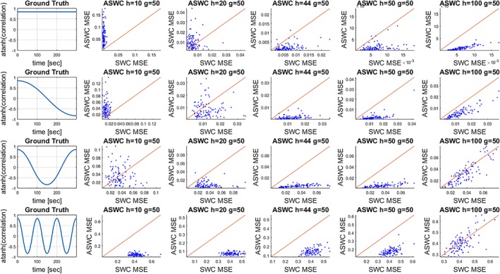
This plot shows the mean square error (MSE) for the ASWC and SWC methods while tracking simulated connectivity dynamics. Four different connectivity dynamics were simulated as representing the ground truth. Time courses were simulated using a cosine summation with randomly selected phases and with phase differences at each time point designed to track the ground truth dynamics. One hundred iterations (each iteration with a different set of random phases) were performed and the MSE displayed for each case. On each ASWC versus SWC plot, a line divides the plotting area in sections where one method has better performance than the other one [Color figure can be viewed at http://wileyonlinelibrary.com]

Simulation results are displayed in Figures 6 and 7. Figure 7 displays the actual estimation at each time point for SWC and ASWC for one of the 100 iterations from Figure 6. A look at the actual estimation in Figure 7 complements the outcomes presented in Figure 6. We included a 44 s window length value from solving (6) for a frequency of 0.01 Hz (0.4441/[0.01 Hz] = 44.41 ≅ 44 s). Averaging length was set using the recommended length g = 1/2f₀ = 50 s. When the connectivity remains approximately constant (the first row in Figure 6 which is the static case), ASWC with window lengths of 44 s and above achieve better performance than a tuned SWC with a window length of 100 s. The case of h_ASWC = 44 s and h_ASWC = 50 s corresponds to ASWC tuned to 0.01 Hz also illustrated in Figure 3 where it was shown to provide better performance than tuned SWC. The first row of Figure 7 allows visualizing how shorter window lengths produce stronger artifacts until ASWC gets properly tuned to a point where the ASWC artifacts are weaker than SWC. For the static case, increasing the window length improves the estimation.

Figure 7.

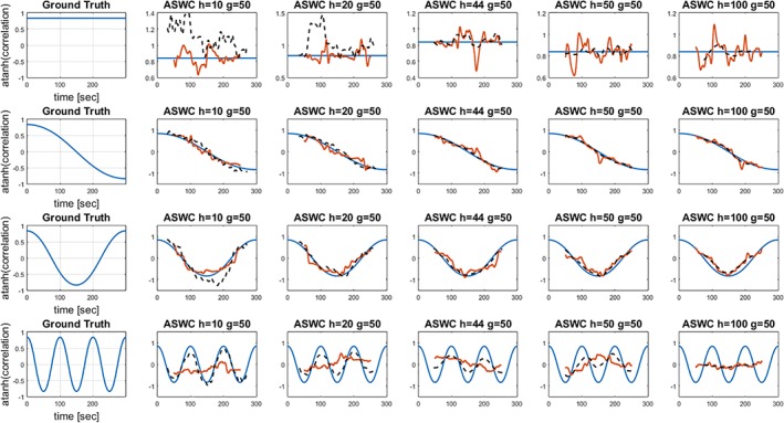
This plot displays one iteration of the simulation from Figure 6. Connectivity estimations for ASWC are displayed by the broken lines in black. Continuous lines in orange represent the SWC estimation. The blue lines represent the ground truth and can be differentiated from the SWC line because they are completely smooth [Color figure can be viewed at http://wileyonlinelibrary.com]

In all other rows of Figure 6, the tuned ASWC case (h_ASWC = 44 s and h_ASWC = 50 s) outperforms SWC. We can explain this by two factors. First, we have shown that tuned ASWC has weaker artifacts than tuned SWC. For the second explanation, we need to take a look at Figure 5 where the phase frequency spectrum response of tuned ASWC with shorter window lengths can resolve higher frequencies than tuned SWC, which requires a larger window length. In other words, as the correlation fluctuates faster, the estimation worsens with a rate that depends on the window length. ASWC has smaller window length and thus results in better performance than SWC.

The last row in Figure 6 shows the results for a dynamic correlation varying with a frequency of 100 Hz. In this case, ASWC outperforms SWC except at the point where SWC and ASWC have the same window length in the last column (h_ASWC = 100 s and h_SWC = 100 s for the last row and last column panel). At shorter window lengths there is more temporal resolution power. The outcome of the last row in Figure 7 shows how the artifacts, although present, are weak for the ASWC method with 10 s window length. As the window length increases, the capability of resolving the 100 Hz frequency diminishes. At the point where h_ASWC = 100 s, both SWC and ASWC show similar performance. This is explained by (10), (12) and Figure 5 in predicting that a correlation frequency of 0.01 Hz cannot be accurately estimated if the window length is 100 s. The last row of Figure 7 illustrates the signal obliteration due to the 100 s window length configured for tuned SWC. As the estimation term ${}_h{}^{\mathit{SWC}}H\left(f\right)\mathrm{\Theta }\left(f\right)$ in (10) is zero at 0.01 Hz, all that we can see during the last row of Figure 7 is the artifact term ${\beth }_h^{\prime }$ of the SWC. When the window length is set to 100 s in the last column and last row of Figure 7, ASWC also exhibits a zero estimation term ${}_g{}^{\mathit{\text{ASWC}}}H\left(f\right){}_h{}^{\mathit{\text{ASWC}}}H\left(f\right)\mathrm{\Theta }\left(f\right)$ from (12) and all that remains is the corresponding artifact term ${\overline{\beth }}_{h,g}^{\prime }$.

3.2. Real data example

Data for this example was borrowed from a previous dynamic connectivity study on polysubstance addiction. We will briefly describe data essentials from the original study, but a more detailed description can be found in Vergara, Weiland, Hutchison, and Calhoun (2018)). Resting state fMRI data were collected on a 3 T Siemens TIM Trio (Erlangen, Germany) scanner. Participants kept their eyes open during the 5‐min resting scan. Echo‐planar EPI sequence images (TR = 2,000 ms, TE = 29 ms, flip angle = 75°) were acquired with an 8‐channel head coil. Each volume consisted of 33 axial slices (64 × 64 matrix, 3.75 × 3.75 mm², 3.5 mm thickness, 1 mm gap). After the necessary preprocessing steps explained in Vergara, Mayer, Damaraju, Hutchison, and Calhoun (2017)) and group independent component analysis, time courses for 39 resting state networks were estimated. All time courses were filtered using a Butterworth band pass filter 0.01 to 0.15 Hz. The SWC technique was then applied with a window length of 100 s. In a separate analysis, the ASWC technique was applied to the filtered time courses with a window length of 44 s and an average length of 50 s. For the 39 retained resting state networks, a total of 741 dynamic functional network connectivity (dFNC) values were estimated for each window. Finally, a k‐means procedure was applied to each technique for SWC and ASWC to detect six different dFNC states in order to identify dFNC state duration, beginning and ending points. We utilized the k‐means clustering outcome to explore the difference between SWC and ASWC. Matching between SWC and ASWC dFNC states was verified by using cross‐correlation with a minimum of 0.997 for paired dFNC states. We used the dFNC states sequence to get an approximation of temporal changes in dFNC. Such changes are not the result of a single SWC from a pair of brain areas, but rather detected using a whole‐brain analysis including 741 pairs of SWC per time point. We assume that dFNC changes from analyzing the whole set are rooted on temporal dFNC variations of the individual SWCs. The dFNC analysis allowed us to find different patterns of temporal dFNC transients to be used as examples.

We pick the three most relevant cases simulated in Figures 6 and 7 static FNC (first row), relatively sharp transition from one dFNC level to a different one (second row), and a periodic dFNC transient where more than one period is available (similar to the fourth row of Figure 7). Interestingly, we found each one of these three cases more than once through the available set of dFNC data. We picked one subject from each case (tuned SWC and tuned ASWC) and one of the 741 FNCs that closely fit the detected dFNC transients. The results are presented in Figure 8 where several observations can be spotted in each case. The standard deviation in the static case is lower in ASWC than SWC similar to the simulation in Figure 3. This outcome in real data is similar to what was observed in the first row of Figure 7, except that true constant correlation is not guaranteed. Yet, fluctuations are weaker for tuned ASWC, indicating a better estimation for this quasi‐static dFNC. The transition case in the second row of Figure 8 exemplifies how these transitions are sharper and suffering from weaker artifacts in ASWC. The sharpness of the estimated transitions can be compared using the differences in slope between ASWC (0.56/[50 s] = 0.0112 s⁻¹) and SWC (0.35/[50 s] = 0.0070 s⁻¹). For comparing the two slopes, we chose a time lapse of 50 s around the 150 s mark where the effect of the transition is prominent and free of artifacts. We also discarded the artifact overshoot occurring in SWC around the 200 s mark as seen in Figure 8. The artifact occurring around 200 s has a weaker amplitude in ASWC, which is consistent with ASWC ability of reducing artifacts for time lapses of approximately constant connectivity. These results closely resemble the outcomes in Figure 4 where a sharp transition was enforced as the ground truth. The last case of rapid fluctuations also shows the advantage of ASWC over SWC. Transient fluctuations were detected with a higher magnitude as predicted by the frequency responses of the MA model. Observed dFNC fluctuations changed at approximately 0.012 Hz. This frequency is close to the zeroing SWC frequency 0.01 Hz (Figure 5); thus, it's strength is highly reduced in SWC estimation. Contrastingly, the strength is higher in ASWC because the zeroing frequency 0.02 Hz is not that close to 0.012 Hz as compared to SWC. This difference between ASWC and SWC also affected the estimated sequence of dFNC states. The sequence of states in ASWC resembles the oscillatory variation of the corresponding ASWC dFNC estimation. However, the SWC state sequence resembles a sharp phase transition in spite of estimating a more oscillatory dFNC. This effect might be a consequence of a sequence of states estimated from a whole‐brain k‐means with weaker signal when compared to ASWC.

Figure 8.

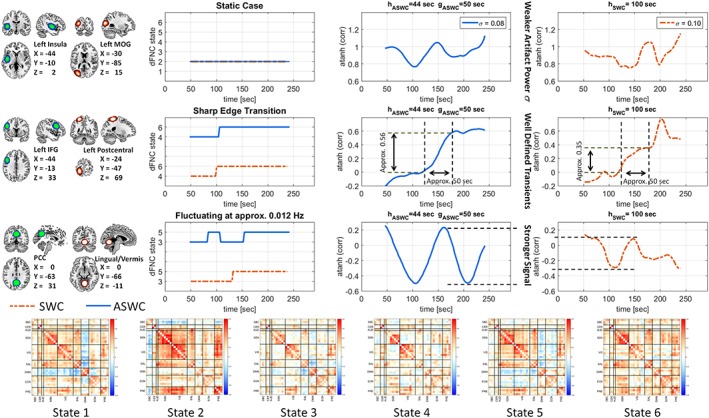
This plot shows several examples from real data. This set of examples closely resembles the simulations in Figure 6 and 7. Although there is no ground truth, we can estimate quasi‐static, quasi‐sharp transitions and fluctuating dFNC using the dynamic state membership functions of each case. Centroid matrices for the six dynamic states are displayed, but a more detailed version is provided in the Supporting Information Appendix S2 Figure. To better illustrate the centroids, brain areas were organized into nine domains: Subcortical (SBC), cerebellum (CER), auditory (AUD), sensorimotor (SEN), visual (VIS), salience (SAL), default mode network (DMN), executive control network (ECN) and precuneus (PRE). Six brain areas are used: Insula, middle occipital gyrus (MOG), inferior frontal gyrus (IFG), postcentral gyrus, posterior cingulate cortex (PCC), and lingual gyrus/cerebellar vermis. Displayed coordinates are in MNI space. Brain areas and dynamic states were extracted from previous work (Vergara et al., 2018). Each row uses data from a different subject where the corresponding pattern was observed. Both SWC and ASWC were tuned to nominal values based on a lower limit frequency of 0.01 Hz. On the static case, ASWC exhibit weaker fluctuations as expected from an appropriate estimation of static connectivity. The single transition case was better defined by ASWC where a smoother and shaper slope was estimated. In the fluctuating dFNC case, ASWC shows a stronger signal than in SWC. The membership function of ASWC was also sensitive to rapid transitions, whereas the SWC membership resembles more the sharp transition case [Color figure can be viewed at http://wileyonlinelibrary.com]

4. DISCUSSION

Several concerns were raised when the first model tracking dynamic connectivity using covariance was made public (Leonardi & Van De Ville, 2015). One controversial assertion was the choice of a window length 1/f₀ according with the lowest frequency f₀ of the BOLD signal. Given that a typical low frequency cutoff is 0.01 Hz, the covariance equation leads to a window length of 100 s (Leonardi & Van De Ville, 2015). As demonstrated by our simulations, a long window length such as 100 s diminishes the ability of accurately resolving the functional connectivity dynamics because of the smoothing nature of performing a correlation over a long period of time. The ASWC method proposed in this work exhibited better performance over SWC at both dFNC extremes: very slow (quasi‐static) and relatively fast temporal fluctuations of connectivity. The cost for ASWC involves an additional processing step that is necessary to perform the averaging in ASWC as compared to SWC, while the pay‐out for this trivial averaging step is a significant improvement in performance.

In addition to proposing a new technique, we have characterized and compared ASWC against SWC through this work. The first model analyzed corresponded to a non‐varying correlation or a static case. This represents the most extreme case of zero fluctuations or frequency zero. The presence of artifacts in the form of spurious fluctuations was the main concern in this static case. Analytical methods predicted artifact reduction in ASWC beyond that obtained with SWC. Real data simulations in Figure 8 corroborate the prediction as fluctuations were weaker in ASWC when no change in dFNC state was estimated. The condition in this case was that averaging length needed tuning using g_ASWC = 1/(2f₀) reducing artifacts for any time‐course frequency f > f₀. Notably, in this static connectivity case time signals can exhibit any frequency while their correlation is constant. Figure 1 shows that complete artifact obliteration is achievable for a single constant sinusoidal signal at f₀. The analysis for frequencies above f₀ revealed a better performance of ASWC over SWC. The simulation in Figure 3 reveals an artifact magnitude of more than 1,000 times larger in SWC compared to ASWC for some frequencies. However, achieving the better performance was dependent on appropriate tuning of the ASWC window length. After analyzing the influence of time signals frequency, it was determined in (6) that the correct tuning was h_ASWC = 0.4441/f₀. This value if about 44.4% times the tuning (h_SWC = 1/f₀) suggested for SWC (Leonardi & Van De Ville, 2015). While the true rewards of a shorter window length in ASWC are not fully observable in the static case, there are obvious advantages in nonstatic cases that we discuss next.

The sharp transition model described sudden changes in connectivity. In this case, the averaging length plays a lesser role. The sharpness resolution is mainly determined by the window length. As tuned h_ASWC is less than half h_SWC, the model roughly predicts twice the ability of resolving sudden changes in connectivity. Simulations in Figure 4 show how doubling the window length, but not the averaging length, doubled the smoothing of the imposed sudden connectivity change. This model does not only describe an idealized situation, but it could also characterize time intervals of quasi‐static dynamic connectivity. These quasi‐static intervals were suggested with the dawn of dynamic connectivity to explain why clustering methods might be able to detect intervals featuring a single dFNC state (Allen et al., 2014). With respect to our current discussion, the quasi‐static case displayed on the second row of Figure 8 was better described by ASWC with better definition of the transition interval and flatter slopes on the quasi‐static extremes. Although the real connectivity is unknown for real data, stronger fluctuations were observed towards the left and right sides of the SWC estimation. As larger artifact fluctuations are expected in SWC for the static connectivity case depicted in Figure 3, we can suspect that SWC lobes not present in ASWC are anything but artifacts.

The most complete description of SWC and ASWC presented in this work was the moving average model (MA model). In this model, we divided the signal in an estimation term and an artifact term. The main interest is to allow for the estimation term to be stronger than the artifact term. In both SWC and ASWC, the estimation terms are described by a moving average system. Moving average systems exhibit a well‐known frequency response which allows making further prediction for SWC and ASWC. The frequencies in the MA model refer to how fast the correlation between two time signals changes, as opposed to the frequency of time signals that were characterized in the static connectivity model. SWC is limited in frequency by the window length which should be tuned to h_SWC = 1/f₀, while ASWC depends on the averaging length tuned at g_ASWC = 1/(2f₀). In simple terms, the MA model indicates that ASWC will resolve faster transients than SWC because the correlation frequency spectrum allows it. Notice that at tuning $\frac{h_{\mathit{SWC}}}{g_{\mathit{\text{ASWC}}}}=2$, ASWC allows for about two times higher frequencies than SWC. Real data and wide‐band simulations agree with this prediction. Figure 7 shows how the simulated ground truth is obliterated in tuned SWC because the correlation fluctuated with a frequency of exactly 1/h_SWC. The fluctuations in this case were related only to the artifact terms of the MA model. Since it is tuned differently, ASWC was able to track the relatively fast simulated changes that SWC could not resolve. The real data example in Figure 8, shows how the connectivity frequency at 0.012 Hz is weaker in SWC compared to ASWC because of its proximity to the zeroing SWC frequency tuned at 0.01 Hz. However, ASWC tuning permits frequencies up to 0.02 Hz (see Figure 5) resulting in a better estimation.

4.1. Limitations

As is the case with other similar studies (Leonardi & Van De Ville, 2015; Zalesky & Breakspear, 2015), the current work does not promise to eliminate all artifact fluctuations, but focuses on reducing their magnitude. Other effects due to the intrinsic characteristics of the hemodynamic response and noise (Hutchison et al., 2013; Lehmann, White, Henson, Cam, & Geerligs, 2017) are not considered in this work. However, ASWC might reduce some of these nuisance effects due to the filtering properties of the MA (Oppenheim & Schafer, 1989).

The improved performance of ASWC over SWC was initially tested through simulations since a ground truth exists for simulated data. A similar attempt to use real data confirmed similar trends as those obtained from simulations. Whether the estimated fluctuations in real data fully represent neuronal activations or are the result of signal nuisances still remains to be confirmed and is a question beyond the topic of this work. However, we might hope that reducing window length artifacts of dFC signals can allow future research in determining ways of cleaning the signal from other nuisances.

4.2. Conclusion

Including an averaging step in the processing of SWC (ASWC) provided a method for reducing artifact fluctuations due to windowing as compared to raw SWC. This reduction in artifacts enhances the ability of the ASWC method to track real dFC fluctuations as compared to the raw SWC method. In contrast to SWC, which requires only setting the window length, there are two parameters to define in ASWC, the window length h_ASWC and the averaging length g_ASWC. The optimal design parameters for ASWC can be written as:

1. Select a design of the lowest allowed frequency f₀ for the time signals to be correlated.

2. Set h_ASWC = 0.4441/f₀ to implement ASWC as a second order high pass filter with cut‐off at f₀.

3. Set g_ASWC = 1/(2f₀) to maximize the reduction of artifacts at f₀ and for higher frequencies f > f₀.

Assuming a cut‐off at f₀= 0.01 Hz, the configuration values are h_ASWC= 44.41 s and g_ASWC= 50 s. Although 50 s seems like a large averaging because g_ASWC + h_ASWC= 94 s, this work showed that temporal resolution depends less on the sum g_ASWC + h_ASWC and is more heavily influenced by the individual lengths g_ASWC and h_ASWC. The important point was to reduce window and averaging lengths (or a combination) for a frequency spectrum that allowed resolving higher frequencies. In summary, an optimally configured ASWC suggests several advantages over the optimal SWC configuration with the recommended length h_SWC= 100 s:

1. A smaller optimal window length h_ASWC = 44.41 s allows for better tracking of temporal dFC fluctuations (Figure 6).

2. The ASWC configuration with h_ASWC= 44.41 s and g_ASWC= 50 s behaves similar to a Butterworth filter at 0.01 Hz, thus aiding in removing nuisance frequencies (Figure 2).

3. Overall, ASWC exhibits less artifact fluctuations when considering a wide range of frequencies of interest at very low frequencies (quasi‐static). See Figure 3 for temporal signals frequency.

4. ASWC presents a correlation frequency spectrum that allows resolving higher frequencies than SWC. See Figure 5 for a comparison of frequency spectrums. See Figures 6 and 7 for simulation results on correlation frequency.

Supporting information

Appendix S1: Supplementary Information.

Appendix S2: Supplementary Figure

Vergara VM, Abrol A, Calhoun VD. An average sliding window correlation method for dynamic functional connectivity. Hum Brain Mapp. 2019;40:2089–2103. 10.1002/hbm.24509

REFERENCES

- Allen, E. A. , Damaraju, E. , Plis, S. M. , Erhardt, E. B. , Eichele, T. , & Calhoun, V. D. (2014). Tracking whole‐brain connectivity dynamics in the resting state. Cerebral Cortex, 24, 663–676. [DOI] [PMC free article] [PubMed] [Google Scholar]
- Allen, E. A. , Erhardt, E. B. , Damaraju, E. , Gruner, W. , Segall, J. M. , Silva, R. F. , … Calhoun, V. D. (2011). A baseline for the multivariate comparison of resting‐state networks. Frontiers in Systems Neuroscience, 5, 2. [DOI] [PMC free article] [PubMed] [Google Scholar]
- Biswal, B. , Zerrin Yetkin, F. , Haughton, V. M. , & Hyde, J. S. (1995). Functional connectivity in the motor cortex of resting human brain using echo‐planar MRI. Magnetic Resonance in Medicine, 34, 537–541. [DOI] [PubMed] [Google Scholar]
- Calhoun, V. D. , Maciejewski, P. K. , Pearlson, G. D. , & Kiehl, K. A. (2008). Temporal lobe and "default" hemodynamic brain modes discriminate between schizophrenia and bipolar disorder. Human Brain Mapping, 29, 1265–1275. [DOI] [PMC free article] [PubMed] [Google Scholar]
- Chang, C. , & Glover, G. H. (2010). Time–frequency dynamics of resting‐state brain connectivity measured with fMRI. NeuroImage, 50, 81–98. [DOI] [PMC free article] [PubMed] [Google Scholar]
- Chang, C. , Liu, Z. , Chen, M. C. , Liu, X. , & Duyn, J. H. (2013). EEG correlates of time‐varying BOLD functional connectivity. NeuroImage, 72, 227–236. [DOI] [PMC free article] [PubMed] [Google Scholar]
- Chen, J. E. , & Glover, G. H. (2015). BOLD fractional contribution to resting‐state functional connectivity above 0.1 Hz. NeuroImage, 107, 207–218. [DOI] [PMC free article] [PubMed] [Google Scholar]
- Cordes, D. , Haughton, V. M. , Arfanakis, K. , Carew, J. D. , Turski, P. A. , Moritz, C. H. , … Meyerand, M. E. (2001). Frequencies contributing to functional connectivity in the cerebral cortex in "resting‐state" data. American Journal of Neuroradiology, 22, 1326–1333. [PMC free article] [PubMed] [Google Scholar]
- Cordes, D. , Haughton, V. M. , Arfanakis, K. , Wendt, G. J. , Turski, P. A. , Moritz, C. H. , … Meyerand, M. E. (2000). Mapping functionally related regions of brain with functional connectivity MR imaging. American Journal of Neuroradiology, 21, 1636–1644. [PMC free article] [PubMed] [Google Scholar]
- Corey, D. M. , Dunlap, W. P. , & Burke, M. J. (1998). Averaging correlations: Expected values and bias in combined Pearson rs and Fisher's z transformations. The Journal of General Psychology, 125, 245–261. [Google Scholar]
- Damoiseaux, J. S. , Rombouts, S. A. , Barkhof, F. , Scheltens, P. , Stam, C. J. , Smith, S. M. , & Beckmann, C. F. (2006). Consistent resting‐state networks across healthy subjects. Proceedings of the National Academy of Sciences of the United States of America, 103, 13848–13853. [DOI] [PMC free article] [PubMed] [Google Scholar]
- Fransson, P. (2005). Spontaneous low‐frequency BOLD signal fluctuations: An fMRI investigation of the resting‐state default mode of brain function hypothesis. Human Brain Mapping, 26, 15–29. [DOI] [PMC free article] [PubMed] [Google Scholar]
- Friston, K. J. , Fletcher, P. , Josephs, O. , Holmes, A. , Rugg, M. D. , & Turner, R. (1998). Event‐related fMRI: Characterizing differential responses. NeuroImage, 7, 30–40. [DOI] [PubMed] [Google Scholar]
- Friston, K. J. , Holmes, A. P. , Poline, J. B. , Grasby, P. J. , Williams, S. C. , Frackowiak, R. S. , & Turner, R. (1995). Analysis of fMRI time‐series revisited. NeuroImage, 2, 45–53. [DOI] [PubMed] [Google Scholar]
- Friston, K. J. , Holmes, A. P. , Price, C. J. , Buchel, C. , & Worsley, K. J. (1999). Multisubject fMRI studies and conjunction analyses. NeuroImage, 10, 385–396. [DOI] [PubMed] [Google Scholar]
- Greicius, M. (2008). Resting‐state functional connectivity in neuropsychiatric disorders. Current Opinion in Neurology, 21, 424–430. [DOI] [PubMed] [Google Scholar]
- Handwerker, D. A. , Roopchansingh, V. , Gonzalez‐Castillo, J. , & Bandettini, P. A. (2012). Periodic changes in fMRI connectivity. NeuroImage, 63, 1712–1719. [DOI] [PMC free article] [PubMed] [Google Scholar]
- Hindriks, R. , Adhikari, M. H. , Murayama, Y. , Ganzetti, M. , Mantini, D. , Logothetis, N. K. , & Deco, G. (2016). Can sliding‐window correlations reveal dynamic functional connectivity in resting‐state fMRI? NeuroImage, 127, 242–256. [DOI] [PMC free article] [PubMed] [Google Scholar]
- Horwitz, B. (2003). The elusive concept of brain connectivity. NeuroImage, 19, 466–470. [DOI] [PubMed] [Google Scholar]
- Xie, H. , Gonzalez‐Castillo, J. , Handwerker, D. A. , Molfese, P. , Bandettini, P. A. , & Mitra, S. (2018). Efficacy of different dynamic functional connectivity methods to capture cognitively relevant information. NeuroImage, 188, 502–514. [DOI] [PMC free article] [PubMed] [Google Scholar]
- Hutchison, R. M. , Womelsdorf, T. , Allen, E. A. , Bandettini, P. A. , Calhoun, V. D. , Corbetta, M. , … Gonzalez‐Castillo, J. (2013). Dynamic functional connectivity: Promise, issues, and interpretations. NeuroImage, 80, 360–378. [DOI] [PMC free article] [PubMed] [Google Scholar]
- Josephs, O. , & Henson, R. N. (1999). Event‐related functional magnetic resonance imaging: Modelling, inference and optimization. Philosophical Transactions of the Royal Society of London. Series B, Biological Sciences, 354, 1215–1228. [DOI] [PMC free article] [PubMed] [Google Scholar]
- Kiviniemi, V. , Kantola, J. H. , Jauhiainen, J. , & Tervonen, O. (2004). Comparison of methods for detecting nondeterministic BOLD fluctuation in fMRI. Magnetic Resonance Imaging, 22, 197–203. [DOI] [PubMed] [Google Scholar]
- Lehmann, B. C. L. , White, S. R. , Henson, R. N. , Cam, C. , & Geerligs, L. (2017). Assessing dynamic functional connectivity in heterogeneous samples. NeuroImage, 157, 635–647. [DOI] [PMC free article] [PubMed] [Google Scholar]
- Leonardi, N. , & Van De Ville, D. (2015). On spurious and real fluctuations of dynamic functional connectivity during rest. NeuroImage, 104, 430–436. [DOI] [PubMed] [Google Scholar]
- Mantini, D. , Perrucci, M. G. , Del Gratta, C. , Romani, G. L. , & Corbetta, M. (2007). Electrophysiological signatures of resting state networks in the human brain. Proceedings of the National Academy of Sciences of the United States of America, 104, 13170–13175. [DOI] [PMC free article] [PubMed] [Google Scholar]
- Oppenheim, A. V. , & Schafer, R. W. (1989). Discrete‐time signal processing (Vol. xv, p. 879). Englewood Cliffs, NJ: Prentice Hall. [Google Scholar]
- Oppenheim, A. V. , & Schafer, R. W. (2010). Discrete‐time signal processing (Vol. xxviii, p. 1108). Upper Saddle River NJ: Pearson. [Google Scholar]
- Preti, M. G. , Bolton, T. A. , & Van De Ville, D. (2017). The dynamic functional connectome: State‐of‐the‐art and perspectives. NeuroImage, 160, 41–54. [DOI] [PubMed] [Google Scholar]
- Sakoglu, U. , Calhoun, V. Dynamic windowing reveals task‐modulation of functional connectivity in schizophrenia patients vs healthy controls; 2009a. p 3675.
- Sakoglu, U. , & Calhoun, V. D. (2009b). Temporal dynamics of functional network connectivity at rest: A comparison of schizophrenia patients and healthy controls. NeuroImage, 47, S169. [Google Scholar]
- Sakoğlu, Ü. , Pearlson, G. D. , Kiehl, K. A. , Wang, Y. M. , Michael, A. M. , & Calhoun, V. D. (2010). A method for evaluating dynamic functional network connectivity and task‐modulation: Application to schizophrenia. Magnetic Resonance Materials in Physics, Biology and Medicine, 23, 351–366. [DOI] [PMC free article] [PubMed] [Google Scholar]
- Schulz, D. , & Huston, J. P. (2002). The sliding window correlation procedure for detecting hidden correlations: Existence of behavioral subgroups illustrated with aged rats. Journal of Neuroscience Methods, 121, 129–137. [DOI] [PubMed] [Google Scholar]
- Shakil, S. , Lee, C. H. , & Keilholz, S. D. (2016). Evaluation of sliding window correlation performance for characterizing dynamic functional connectivity and brain states. NeuroImage, 133, 111–128. [DOI] [PMC free article] [PubMed] [Google Scholar]
- Silver, N. C. , & Dunlap, W. P. (1987). Averaging correlation coefficients: Should Fisher's z transformation be used? Journal of Applied Psychology, 72, 146–148. [Google Scholar]
- Toro, R. , Fox, P. T. , & Paus, T. (2008). Functional coactivation map of the human brain. Cerebral Cortex, 18, 2553–2559. [DOI] [PMC free article] [PubMed] [Google Scholar]
- Vergara, V. M. , Mayer, A. R. , Damaraju, E. , Hutchison, K. , & Calhoun, V. D. (2017). The effect of preprocessing pipelines in subject classification and detection of abnormal resting state functional network connectivity using group ICA. NeuroImage, 145, 365–376. [DOI] [PMC free article] [PubMed] [Google Scholar]
- Vergara, V. M. , Weiland, B. J. , Hutchison, K. E. , & Calhoun, V. D. (2018). The impact of combinations of alcohol, nicotine, and cannabis on dynamic brain connectivity. Neuropsychopharmacology, 43, 877–890. [DOI] [PMC free article] [PubMed] [Google Scholar]
- Wilson, R. S. , Mayhew, S. D. , Rollings, D. T. , Goldstone, A. , Przezdzik, I. , Arvanitis, T. N. , & Bagshaw, A. P. (2015). Influence of epoch length on measurement of dynamic functional connectivity in wakefulness and behavioural validation in sleep. NeuroImage, 112, 169–179. [DOI] [PubMed] [Google Scholar]
- Woodward, N. D. , & Cascio, C. J. (2015). Resting‐state functional connectivity in psychiatric disorders. JAMA Psychiatry, 72, 743–744. [DOI] [PMC free article] [PubMed] [Google Scholar]
- Zalesky, A. , & Breakspear, M. (2015). Towards a statistical test for functional connectivity dynamics. NeuroImage, 114, 466–470. [DOI] [PubMed] [Google Scholar]
- Zalesky, A. , Fornito, A. , Cocchi, L. , Gollo, L. L. , & Breakspear, M. (2014). Time‐resolved resting‐state brain networks. Proceedings of the National Academy of Sciences, 111, 10341–10346. [DOI] [PMC free article] [PubMed] [Google Scholar]
Associated Data
This section collects any data citations, data availability statements, or supplementary materials included in this article.
Supplementary Materials