Omission of temporal nuisance regressors from dual regression can improve accuracy of fMRI functional connectivity maps

Abstract

Functional connectivity (FC) maps from brain fMRI data can be derived with dual regression, a proposed alternative to traditional seed‐based FC (SFC) methods that detect temporal correlation between a predefined region (seed) and other regions in the brain. As with SFC, incorporating nuisance regressors (NR) into the dual regression must be done carefully, to prevent potential bias and insensitivity of FC estimates. Here, we explore the potentially untoward effects on dual regression that may occur when NR correlate highly with the signal of interest, using both synthetic and real fMRI data to elucidate mechanisms responsible for loss of accuracy in FC maps. Our tests suggest significantly improved accuracy in FC maps derived with dual regression when highly correlated temporal NR were omitted. Single‐map dual regression, a simplified form of dual regression that uses neither spatial nor temporal NR, offers a viable alternative whose FC maps may be more easily interpreted, and in some cases be more accurate than those derived with standard dual regression.

1. INTRODUCTION

Brain functional connectivity (FC), broadly defined as coactivation of brain regions (Huettel, Song, & McCarthy, 2014), is commonly derived with fMRI seed‐based FC (SFC) methods that assess temporal correlations between blood‐oxygen‐level‐dependent activity in a selected seed region, with that of voxels in other brain regions (Biswal, Yetkin, Haughton, & Hyde, 1995; Fox et al., 2005; Friston, 2002; Huettel et al., 2014; Van Dijk et al., 2010). z‐Score maps that reflect FC at each voxel can be derived from these correlations for comparison of FC across individual subjects and/or fMRI sessions (Biswal et al., 2010; Fox et al., 2005; Smith et al., 2014). Multiple regression can facilitate this derivation via the general linear model (GLM) (Huettel et al., 2014; Kelly et al., 2010; McKeown, 2000; Smith et al., 2014; Worsley & Friston, 1995). When approximate time courses for noise sources are available, such as from movement or respiration, their inclusion in the GLM as nuisance regressors (NR) may improve the accuracy of derived FC maps (Birn, 2012; Birn, Murphy, Handwerker, & Bandettini, 2009; Power et al., 2014; Power, Schlaggar, & Petersen, 2015; Satterthwaite et al., 2013; Van Dijk et al., 2010; Yan et al., 2013). Appropriate choices for such NR are the subject of much discussion, as NR can often significantly impact regression coefficient estimates of regressors of interest (Bright, Tench, & Murphy, 2017; Caballero‐Gaudes & Reynolds, 2017; Murphy, Birn, Handwerker, Jones, & Bandettini, 2009; Murphy & Fox, 2017; Satterthwaite et al., 2013), and poor choices may reduce the sensitivity of detecting task‐related changes (Aguirre, Zarahn, & D'Esposito, 1998; Chen et al., 2012; Ciric et al., 2017; Griffanti et al., 2014; Murphy, Birn, & Bandettini, 2013).

Dual regression has been introduced as an alternative to conventional SFC (Beckmann, Mackay, Filippini, & Smith, 2009), with the potential for improving the accuracy of FC maps over those derived with SFC (Smith et al., 2014). Dual regression utilizes the GLM in two regression steps: First, a set of spatial priors is regressed onto fMRI data from individual subjects (or sessions, for multiple sessions per subject). These spatial priors can be whole‐brain spatial maps taken from any source, for example, from previous studies or constructed based on theoretical considerations (Biswal et al., 2010; Kelly et al., 2010), but as originally proposed (Beckmann et al., 2009) these maps are derived from a group independent component analysis (ICA) involving all subjects/sessions whose FC maps are to be compared. Second, the time courses derived from the first step are regressed onto the fMRI data from the corresponding subjects/sessions to yield FC maps. Each spatial prior used as input to the dual regression process corresponds directly to a single time course and FC map for each fMRI session. If one of the spatial priors is considered to represent a “network” (constellation of coactivated regions of the brain) to be studied, then the corresponding time courses and FC maps for each subject/session also represent the network of interest. Other networks, whether considered signals of potential interest or noise, represent variance that is parsed separately in regression from the spatial map and signal of interest, so their spatial priors and time courses can be considered “NR” (Figure 1). The temporal regression is analogous to application of the GLM with SFC, where the time course for the signal of interest in dual regression is obtained by regressing the spatial prior of interest onto the fMRI data, rather than by averaging time courses of voxels in a seed region; and the remaining, nuisance‐regressor time courses correspond to spatial priors representing neural signals or structured (non‐Gaussian) noise (Beckmann, 2012).

Figure 1.

Illustration of dual regression, mapping visual cortex FC for a selected subject. The full set of spatial priors (in this example, N spatial maps from group ICA of all subjects' conventionally preprocessed, temporally concatenated fMRI data) is regressed onto the fMRI data for subject i, yielding time courses that are in turn regressed onto subject i's fMRI data to yield a set of FC maps. One of the group‐derived spatial priors is identified as representing the network of interest (visual cortex), and its corresponding FC map represents FC for subject i's visual cortex. In standard dual regression (DRA, dual regression with all regressors), if we are only interested in the visual cortex component, then the remaining FC maps are ignored, as maps of no interest. In our study, we consider SMDR, a variant of dual regression where nuisance regressors are completely omitted from both regressions. FC, functional connectivity; ICA, independent component analysis; SMDR, single‐map dual regression [Color figure can be viewed at http://wileyonlinelibrary.com]

As with SFC, NR applied with dual regression require careful consideration to prevent negatively impacting the accuracy of derived FC maps. Inclusion of NR in dual regression could theoretically increase the accuracy of FC maps by regressing out structured noise (Kelly et al., 2010), ensuring that residuals are Gaussian (as is typically assumed by the regression estimation procedure), and by appropriately parsing variance originating from spatially overlapping neural signal sources, to each source separately (Leech, Kamourieh, Beckmann, & Sharp, 2011; Smith et al., 2014; Smith, Sip, & Delgado, 2015). However, in one study based on task‐fMRI data, omission of NR from dual regression actually increased correlations of derived FC maps with GLM‐derived maps based on an a priori time course derived from the task paradigm, prompting investigators to question whether in some cases more accurate FC maps can be derived by omitting NR from dual regression (Kelly et al., 2010). Here, we demonstrate that such omission of NR can improve accuracy of FC derived with dual regression, because standard dual regression can introduce spurious signal of interest into NR, potentially causing them to become more highly correlated (or anticorrelated) with the signal of interest.

Spuriously high correlations can be induced by the ubiquitous misalignments across subjects that result in correlations between the spatial distribution of signal of interest and nuisance spatial priors. Although mapping of functionally homologous brain areas across subjects has improved (Glasser, et al., 2013; Glasser et al., 2016; Gordon et al., 2016; Gordon, Laumann, Adeyemo, & Petersen, 2017; Laumann et al., 2015; Mueller et al., 2013; Satterthwaite & Davatzikos, 2015; Smith et al., 2013), spatial distributions for neural networks and structured noise in individual subjects cannot be expected to align themselves perfectly with their corresponding group ICA components, due to (a) functional differences in brain activity patterns across subjects (Duncan, Pattamadilok, Knierim, & Devlin, 2009; Gordon et al., 2016; Gordon et al., 2017; Gorgolewski et al., 2013; Laumann et al., 2015; Mueller et al., 2013; Satterthwaite & Davatzikos, 2015; Saxe, Brett, & Kanwisher, 2006); (b) inaccuracies in brain alignment during normalization to standard brain space (Ardekani et al., 2005; Klein et al., 2009; Morey et al., 2009); and (c) incomplete representation of the full spatial extent of the neural network of interest, as can happen if ICA represents one functional network with two or more smaller components (Abbott, Il, Bustillo, & Calhoun, 2010; Beckmann, DeLuca, Devlin, & Smith, 2005; Birn, Murphy, & Bandettini, 2008; Cardinale, Shih, Fishman, Ford, & Muller, 2013; Lin, Liu, Zheng, Liang, & Calhoun, 2010; McKeown et al., 1998; Ylipaavalniemi & Vigario, 2008; Zuo et al., 2010). Spatial regression translates these spatial correlations into temporal correlations between the time course of interest and derived nuisance time courses, which in turn can reduce the accuracy of the FC map of interest (MOI) derived from temporal regression (Figure 2).

Figure 2.

Vector‐space illustration of spurious correlations that arise during spatial regression, between temporal nuisance regressors and signal of interest, as a consequence of “misalignments” between nuisance spatial priors and the spatial distribution of signal of interest (see text for details). Consider three mutually uncorrelated spatial distributions (+1 or −1 in areas A1, A2, and A3) for mutually uncorrelated signals S ₁, S ₂, and S ₃, respectively. When spatial priors P ₁, P ₂, and P ₃ correlate perfectly with spatial distributions of their corresponding signals in fMRI data (Case A), then each time course derived from spatial regression (T _a1, T _a2, and T _a3) approximates its corresponding signal in the fMRI data (S ₁, S ₂, and S ₃). However, when “overlap” (spatial correlation) exists between a nuisance spatial prior and the distribution of signal of interest (Case B), then the time course derived from the nuisance spatial prior (T _b2) will tend to correlate with the signal of interest (S ₁). This spurious correlation with the signal of interest can increase dramatically when the nuisance spatial prior has no corresponding signal from structured noise or neural signal of no interest in the fMRI data (Case C): In the absence of the nuisance signal (S ₂), the signal of interest can become the largest component of the derived nuisance time‐course vector (T _c2)

To illustrate these effects, we compared the accuracy of FC maps derived with two variants of dual regression: one using all spatial maps from a group ICA as the spatial priors (DRA: standard dual regression with all spatial maps), and one using a single map from the group ICA as the only spatial prior (single‐map dual regression [SMDR]). We performed these comparisons using (a) resting‐state data, to which we added artificial signals with known spatial distributions to provide accurate standard‐of‐comparison (SOC) maps to assess FC‐map accuracy; and (b) task‐fMRI data, to study our methods with unaltered fMRI data, through SOC maps that are derived from GLM using a priori time courses. We also explored mechanisms responsible for differences in FC‐map accuracy as they relate to collinearity between signal of interest and temporal NR.

2. THEORY

To simplify the analysis, we consider the goal of deriving a single FC map, corresponding to a single signal of interest, via dual regression. Regressors that do not correspond to the designated signal of interest are considered NR.

2.1. Regression

Our linear regression procedures are based on the equation

$$\mathbf{Y}={\mathrm{b}}_1{\mathbf{X}}_{\mathbf{1}}+{\mathrm{b}}_2{\mathbf{X}}_{\mathbf{2}}+{\mathrm{b}}_3{\mathbf{X}}_{\mathbf{3}}+\dots +{\mathrm{b}}_{\mathrm{n}}{\mathbf{X}}_{\mathbf{n}}+\mathrm{c}+\mathbf{\epsilon },$$ (1)

where the best approximation for the values of vector Y (the dependent variable, representing the spatial map for a given time point or the vector time course for a given voxel) for a given set of vectors {X ₁, X ₂, … X _n} (n independent variables, representing either spatial maps or time courses) is found by choosing the set of regression coefficients {b₁, b₂, … b_n} that minimize the sum of squares of the residual values in vector ε. We say that the independent variables are being regressed onto the dependent variable, borrowing terminology from Huettel et al. (2014), recognizing that no consensus for such terminology yet exists in the dual regression literature (Abram et al., 2017; Baggio et al., 2015; Chahine, Richter, Wolter, Goya‐Maldonado, & Gruber, 2017; Geissmann et al., 2018; Ishaque et al., 2017; Muetzel et al., 2016; Odish et al., 2015; Pannekoek et al., 2015; Smith et al., 2015). Our dependent and independent variables are always mean centered prior to regression (making the terms orthogonal and uncorrelated synonymous); and to ensure that mean values for independent variables predict the mean value for the dependent variable, c is set to zero. Fully filtered fMRI data are produced by finding values (with least‐square linear regression) for independent variable terms on the right‐hand side of the equation and subtracting them from Y, the unfiltered fMRI data. Partially filtered fMRI data are produced in the same way, except that at least one of the terms on the right side of the equation (typically representing the signal of interest) is not subtracted from Y.

Step‐wise partial regression, as defined in this article, is an alternative process for performing regression of a signal of interest and temporal NR onto fMRI data: Temporal NR are first partially filtered from fMRI data

$${\mathbf{Y}}_{\mathbf{p}}=\mathbf{Y}-\left({\mathrm{b}}_2{\mathbf{X}}_{\mathbf{2}}+{\mathrm{b}}_3{\mathbf{X}}_{\mathbf{3}}+\dots +{\mathrm{b}}_{\mathrm{n}}{\mathbf{X}}_{\mathbf{n}}\right),$$ (2)

which are then used in the regression

$${\mathbf{Y}}_{\mathbf{p}}={\mathrm{b}}_{1\mathrm{p}}{\mathbf{X}}_{\mathbf{1}}+{\mathbf{\epsilon }}_{\mathbf{p}}.$$ (3)

Because the right‐hand sides of Equations 2, 3 are equal, the value of b _1p that minimizes the sum of squares of residuals in Equation 3 must equal the value of b ₁ derived from regression Equation 1; and ε _p = ε. However, corresponding FC maps will differ: The t‐score, (regression coefficient)/(SE of regression coefficient), for each voxel derived from Equation 3 is increased relative to that derived from Equation 1, by dropping the NR of Equation 1 that increases the variance of the estimate of the SE of b ₁, by the same factor for every voxel. Thus, the t‐score map derived from Equation 3 becomes a scaled‐up, perfectly correlated version of the t‐score map derived from Equation 1. The resulting FC, z‐score map derived from Equation 1 will not correlate perfectly with the z‐score map derived from Equation 3, because the mapping from t‐scores to z‐scores is nonlinear. Generally, Equation 3 will yield FC maps with higher peak z‐score values, but lower ratios between z‐score peaks and corresponding z‐score SD.

The t‐score derived from Equation 3, t _SNR = b _1p/(SE of b _1p), with df = n−2 (where n is the number of time points) can help to determine the variance in Y _p that is explained by time course X ₁, relative to residual noise, that is, the signal‐to‐noise ratio (SNR) = r ²/(1‐r ²), where r is Pearson's correlation coefficient between Y _p and X ₁. t _SNR = r*sqrt(df/[1‐r ²]) (Glass & Stanley, 1970), so SNR = t _SNR ²/df. For our purposes, t _SNR is more useful than SNR as a measure of the relative strength of signal compared with noise, because t _SNR becomes negative when X ₁ becomes anticorrelated with Y _p.

2.2. Mechanisms affecting FC map accuracy

Figure 2 provides a vector‐space illustration of the primary mechanism that we hypothesize can profoundly decrease accuracy of FC maps derived with standard dual regression: Correlations between the spatial distribution of signal of interest and nuisance spatial priors (“misalignments”) spawn spurious correlations between the signal of interest and derived nuisance time courses.

We consider three cases (A, B, and C) of standard dual regression performed on (preprocessed) fMRI data, using mean‐centered and mutually orthogonal spatial priors, vectors P ₁, P ₂, and P ₃, where P ₁ has value 1 for voxels within area A1+ (top, left) and −1 within area A1−; P ₂ is 1 within A2+ and −1 within A2−; P ₃ is 1 within A3+ and −1 within A3−; and each spatial prior has value 0 elsewhere. Let y _ij represent the value of voxel i at time point j. Equation SR represents the spatial regression, where Ys _j is the vector of y _ij values at time point j, and εs _j is the vector of residuals whose sum of squares is minimized to yield regression coefficients t _1j, t _2j, and t _3j. These regression coefficients over all time points form time‐course vectors T ₁, T ₂, and T ₃ for the temporal regression, represented by Equation TR, where Yt _i is the vector of y _ij values at voxel i, and εt _i is the vector of residuals whose sum of squares is minimized to yield regression coefficients f _1i, f _2i, and f _3i. These regression coefficients over all voxels form FC maps F ₁, F ₂, and F ₃, respectively. Let us consider P ₁ our spatial prior MOI and P ₂ and P ₃ nuisance‐regressor maps; and then F ₁ becomes our FC MOI and F ₂ and F ₃ are ignored.

For Case A, we consider fMRI data formed by adding to random, Gaussian background noise (assumed to be negligible in amplitude for purposes of illustration) the outer products of three orthogonal, mean‐centered time‐course vectors S ₁, S ₂, and S ₃ with maps P ₁, P ₂, and P ₃, respectively. Regression of the spatial maps P ₁, P ₂, and P ₃ onto these fMRI data with equation SR yields coefficients t _1j = s _1j, t _2j = s _2j, and t _3j = s _3j (where s _1j, s _2j, and s _3j, are the jth values of S ₁, S ₂, and S ₃, respectively), because the spatial maps for the distributions of added signals are perfectly correlated with their corresponding spatial prior and uncorrelated with the other spatial priors. If we let vectors T _a1, T _a2, and T _a3 represent the collected values over all j of t _1j, t _2j, and t _3j, respectively, then T _a1, T _a2, and T _a3 will align themselves perfectly in vector space with S ₁, S ₂, and S ₃ (Figure 2, bottom, left); and in this ideal case, nuisance‐regressor time courses T _a2 and T _a3 would not correlate with the signal of interest (S ₁).

For Case B, we repeat the analysis for Case A, beginning with fMRI data that are altered to introduce minor “misalignments” between spatial priors and corresponding spatial distributions of signals within the data: Instead of multiplying S ₁ by P ₁, we multiply it by spatial map Q ₁, which is the same as P ₁, but has value 1 for voxels within area B1+ (Figure 2, top, right) and −1 within equally sized area B1−; and instead of multiplying S ₃ by P ₃, we multiply it by spatial map Q ₃, which is the same as P ₃, but has value 1 for voxels within area B3+, and −1 within equally sized area B3−. Regression with equation SR yields time‐course vectors T _b1, T _b2, and T _b3 (Figure 2, bottom, middle). In this case, the spatial distribution for signal S ₁ (spatial map Q ₁) correlates slightly with P ₂, so T _b2 will not be collinear with S ₂, but shifted by a small angle (θ₂) toward S ₁ in the plane spanned by vectors S ₁ and S ₂. Likewise, the small correlation between spatial map Q ₃ and P ₁ will cause T _b1 to be shifted by a small angle (θ₁) from S ₁ toward S ₃ in the plane spanned by vectors S ₁ and S ₃. Thus, these small deviations in spatial distributions of signals from their corresponding spatial priors cause the signal of interest (S ₁) to become less than perfectly correlated with the time course of interest (T _b1) and slightly correlated with a nuisance time course (T _b2).

The size of this latter correlation can be increased, not only by increasing the spatial correlation between maps Q ₁ and P ₂, but also by decreasing the amplitude of S ₂: For Case C, we repeat Case B, except that we set S ₂ = 0 for all time points (simulating the effect of denoising or nonexistence of S ₂ for a particular subject) and we drop spatial prior P ₃ from the dual regression (simulating the case where P ₃ represents a structured noise source that does not have sufficient variance to be represented in a group ICA, for example, due to involving a relatively small brain area or existing in only one subject). The absence of signal S ₂ in the fMRI data would cause T _c2 to align itself with S ₁ (Figure 2, bottom, right), possibly (depending upon influences from other sources of structured noise and background noise) resulting in substantial signal loss due to regressing out signal of interest. Some signal of interest would end up represented in the ignored FC map F ₂ rather than F ₁. Ironically, any algorithm that removes structured noise sources in a preprocessing step could worsen FC map quality through this mechanism, unless the spatial priors corresponding to the removed noise sources are omitted from the dual regression (e.g., spatial priors generated from a group ICA performed after the denoising would no longer represent noise sources that had been consistently removed for all subjects).

DRA's inclusion of the regressor for the derived signal of interest together with NR in the temporal regression (i.e., partial regression) does not prevent the NR from regressing out most or all of the signal of interest. Addition of a relatively small amount of signal of interest to a nuisance regressor (Case B) can induce an enormous loss of derived FC for the signal of interest, depending upon the other signals that form components of the nuisance regressor (T _b2). Figure 3 illustrates this point with a case where FC is derived with dual regression for a single voxel, whose time course has 15% variance from a neural signal of interest and the rest from two noise sources, one of which is represented in a nuisance regressor for the temporal regression. When this nuisance regressor is uncorrelated with the signal of interest, including it in the regression increases the FC z‐score for the signal of interest; but the addition of relatively small amounts of signal of interest to the nuisance regressor decreases the z‐score to the point of becoming negative, even though the derived signal of interest correlates highly with the true signal of interest.

Figure 3.

Addition of relatively small amounts of signal of interest to temporal NR in dual regression can filter out the signal of interest, causing dramatic reductions in derived FC. Shown in the figure are results of temporal regression using variables S _i (signal of interest), S _n1 (noise source), S _n2 (noise source), S _v (voxel's time course, with 15% of variance from S _i, 60% from S _n1, and 25% from S _n2), and S _d (time course representing the signal of interest, as derived from spatial regression, with 95% of variance from S _i and 5% from S _n1). When NR are omitted from the temporal regression (Equation 1, where c is a constant and ε represents residuals, whose sum of squares is minimized to derive the regression coefficient, b_d), regressing the derived signal of interest (S _d) onto the fMRI data (S _v) yields an FC z‐score of 7.54, corresponding to one‐tailed probability 2.27 × 10⁻¹⁴, derived from the t‐score of b_d/(SE of b_d) = 8.29, with df = 158. This z‐score is increased to 8.58 (corresponding to t‐score of 9.71, with df = 157) when nuisance regressor S _r is incorporated into the regression (Equation 2), if S _r's proportion (P) of variance contributed by S _i is zero. However, small amounts of added signal of interest (S _i) to S _r cause a dramatic drop in the FC z‐score (figure, bottom). When S _i constitutes 20% of S _r's variance, the z‐score is reduced to zero; and higher percentages cause the z‐score to become negative. S _i, S _n1, and S _n2 here are mean centered, mutually orthogonal, and of unit variance. All waveforms are drawn to scale, simulating time courses for 160 volumes of fMRI data. FC, functional connectivity; NR, nuisance regressors

In summary, the spatial regression step of standard dual regression can introduce into derived temporal NR spurious correlations with the signal of interest. These spurious correlations can become large, even larger than the correlation between the derived signal of interest and the true signal of interest, when misalignments occur between nuisance spatial priors and the spatial distributions of their intended signal sources. In addition, relatively small spurious correlations can greatly impact FC accuracy for some voxels when the mix of signal of interest and other signal sources in NR causes the NR to become highly correlated with voxel time courses.

3. MATERIALS AND METHODS

3.1. Overview

To empirically validate these theoretical considerations, performance of SMDR relative to DRA was evaluated in three main experiments, based on how well FC maps (z‐score) agreed with a known SOC map. Our primary measure of agreement was CC, the Pearson's correlation coefficient between FC map and SOC (Figure 4). We chose this commonly used, scaling‐independent measure because it is independent of factors that can elevate the number of voxels selected at any given threshold, including autocorrelation (Davey, Grayden, Egan, & Johnston, 2013; Friston et al., 1995; Woolrich, Ripley, Brady, & Smith, 2001), global signal (Satterthwaite et al., 2013), and structured noise (Satterthwaite et al., 2012; Van Dijk, Sabuncu, & Buckner, 2012). In some cases, we added a secondary measure of agreement, PD, the proportion of voxels within a selected region of the SOC (a binary map representing “true” voxels, from maximum‐height thresholding the SOC) that are detected in the FC map after thresholding the FC map to make the number of false positive and false negative voxels equal (Kelly et al., 2010). PD has the advantage of being invariant under monotonic transformations that do not alter the order of voxels ranked according to voxel values (e.g., unaffected by mapping from t‐scores to z‐scores).

Figure 4.

Overview of method comparison [Color figure can be viewed at http://wileyonlinelibrary.com]

To assess the relationship between FC map accuracy and potential for signal loss due to regressing out signal of interest with DRA, we compared measures of performance to measures of collinearity between the true signal of interest (T _i) and the set of DRA's temporal NR (T _n), using the coefficient of multiple correlation R(T _i,T _n), where function R(X,Y) represents the correlation between the vector variable of interest X and its best, least‐square approximation formed from a linear combination of vector variables in the set Y. To assess the contribution of spatial “misalignments” to increased collinearity between signal of interest and temporal NR, we tested for a relationship between R(T _i,T _n) and R(S _i,S _n), where S _i is the spatial map of the distribution of signal of interest and S _n is the set of nuisance‐regressor spatial prior maps.

In Experiment 1, we simulated a condition where the signal of interest should not be highly correlated with nuisance‐regressor time courses, by adding to resting‐state data an artificial signal of interest that was largely uncorrelated with signals within the data (as defined by component time courses derived from individual‐subject ICA). In Experiment 2, we simulated a contrasting situation, by repeating Experiment 1 with an artificial signal that was highly correlated (r ~ .7) with one of the ICA‐derived component time courses for each subject. Experiment 3 was our natural condition, using task‐fMRI data. For this experiment, the relationship between R(T _i,T _n) and R(S _i,S _n) was not assessed because the distributions of the signals of interest were unknown.

To demonstrate denoising effects, parts of Experiments 1 and 2 were repeated after first denoising the fMRI data using a subset of time courses from single‐subject ICA that were selected with visual inspection (visual inspection, ICA‐based denoising [VIID] (Kelly et al., 2010)), or using all time courses from single‐subject ICA, except for the time course that represents the signal of interest. To facilitate the analysis of the effect of DRA's NR on derived FC maps, we compared these results with those from SMDR, DRA, and DRA performed via step‐wise regression.

3.2. Participants and selection of downloaded data

All procedures were approved by local Institutional Review/Ethics Boards.

3.2.1. Experiments 1 and 2

Publicly available resting‐state fMRI data were downloaded through the 1,000 Functional Connectomes Project (http://www.nitrc.org/projects/fcon_1000) Milwaukee‐B dataset (Biswal et al., 2010), from 46 adult participants. We chose this dataset based on the criteria TR = 2, minimum of 5 min of run time, and approximately 40 subjects—striking a balance between sufficient statistical power and computation time.

A default mode (DM) binary spatial map from previously published studies (Greicius et al., 2007; Kelly et al., 2010) was utilized (Greicius' default mode map [GDMM]), derived from a study of 14 healthy right‐handed adults (Greicius, Srivastava, Reiss, & Menon, 2004).

3.2.2. Experiment 3

Publicly available data were downloaded through the fMRI Data Center (http://www.fmridc.org/, accession number 2‐2003‐114E5) from a study of 14 healthy, right‐handed adults (Haaland, Elsinger, Mayer, Durgerian, & Rao, 2004). This study met our requirement for involving a highly repetitive visuomotor task with activation of sufficiently large portions of the brain to be detected reliably with ICA (Kelly et al., 2010).

3.3. Experimental designs for data collection

3.3.1. Experiments 1 and 2

Six minutes of resting‐state fMRI data were collected from subjects instructed to close their eyes and relax inside the scanner.

3.3.2. Experiment 3

FMRI data were used from a study of the association between brain hemispheric lateralization patterns and motor task complexity (Haaland et al., 2004). Eight runs were collected in that study, with each run involving either a complex or a simple motor task using either the right or left hand; two runs were collected for each of these four cases. Each run involved 10, 24‐s‐long blocks. Each block involved 12 s rest followed by 4, 3‐s trials. The complex condition consisted of heterogeneous sequences of digits, which always used three fingers and four transitions, whereas the simple condition involved repetition of the same digit in each trial.

We used only data from the complex condition because we reasoned that it would offer a more repetitive scenario (all three fingers in every trial), involving brain activity patterns that could be captured equally well with (a) regression of an a priori time course onto the fMRI data and (b) ICA, because the fraction of the overall fMRI variance contributed by this brain activity would rise to a level that would be easily detectable with ICA (Kelly et al., 2010). Thus, four runs from 14 subjects were available for this experiment, two per hand.

3.4. Data acquisition

3.4.1. Experiments 1 and 2

Resting‐state fMRI data were acquired on a 3T GE SIGNA scanner with a standard transmit–receive head coil, using a single‐shot gradient echo‐planar (EP) imaging pulse sequence with TR = 2 s, TE = 25 ms, flip angle 90°, 180 volumes, 36 contiguous sagittal 4‐mm‐thick slices per volume, field‐of‐view (FOV) = 24 × 24 cm², acquisition matrix 64 × 64, and voxel size = 3.75 × 3.75 × 4 mm³. High‐resolution SPGR 3D axial T1‐weighted images were acquired with TR = 10 ms, TE = 4 ms, TI = 450 ms, flip angle = 12°, 144 slices, slice thickness = 1.0 mm, and acquisition matrix 256 × 192.

3.4.2. Experiment 3

Images were acquired using a 1.5T GE SIGNA scanner. EP images were collected using a single‐shot, blipped, gradient‐echo EP pulse sequence with TR = 4 s, TE = 40 ms, 22 contiguous sagittal 6‐mmthick slices, FOV = 24 × 24 cm², 64 × 64 matrix, and voxel size = 3.75 × 3.75 × 6 mm³. High‐resolution 3D spoiled gradient‐recalled at steady‐state anatomic images were collected with TR = 24 ms, TE = 5 ms, flip angle = 40°, number of excitations = 1, slice thickness = 1.2 mm, FOV = 24 cm, resolution = 256 × 128.

3.5. Image preprocessing

FMRI image preprocessing for all experiments was carried out using FSL (version 5.0), FMRIB's Software Library (http://www.fmrib.ox.ac.uk/fsl) (Jenkinson, Beckmann, Behrens, Woolrich, & Smith, 2012; Smith et al., 2004; Woolrich et al., 2009), involving nonbrain removal (Smith, 2002); motion correction (Jenkinson, Bannister, Brady, & Smith, 2002); high‐pass temporal filtering using Gaussian‐weighted least‐squares straight line fitting with σ = 100 s; spatial smoothing using a Gaussian kernel with full‐width half‐maximum 6 mm for Experiments 1 and 2, and 8 mm for Experiment 3; coregistration to high‐resolution T1‐weighted images; and normalization of all images to standard space (Montreal Neurological Institute atlas, using resolutions of 3 × 3 × 3 mm³ for Experiments 1 and 2 and 4 × 4 × 4 mm³ for Experiment 3) with affine registration (Jenkinson et al., 2002; Jenkinson & Smith, 2001). To allow for T1 equilibrium, the first five volumes of resting‐state data and first two volumes of task‐fMRI data were discarded. Resting‐state data from only 45 subjects in Experiments 1 and 2 were used because of excessive motion in one of the resting‐state data runs (mean framewise displacement >0.2 mm).

3.6. Independent component analysis

3.6.1. Experiments 1 and 2

Single‐subject ICA and group ICA were performed with probabilistic ICA (PICA) (Beckmann & Smith, 2004), which can be considered a variant of FastICA (Hyvarinen, 1999) where spatially independent components are estimated simultaneously rather than one at a time. PICA generates statistically meaningful z‐score maps by adding a term representing Gaussian, nonstructured noise to the classic noise‐free ICA framework, and dividing each voxel's raw IC estimate by its corresponding noise SD. Dimensionality was estimated using the Laplace approximation (Beckmann & Smith, 2004; Minka, 2000). Estimated component maps were converted to z‐scores by dividing by the SD of the residual noise and thresholded conservatively (alternative hypothesis test at p > .95) for display, fitting a mixture model to the histogram of intensity values. For group ICA, data from all subjects were temporally concatenated using FSL's Multivariate Exploratory Linear Decomposition into Independent Components (MELODIC) version 3.14. We set the MELODIC epsilon parameter (error tolerance) to 10⁻⁸, because we found in a previous study (Kelly et al., 2010) that using such a low value improved the reproducibility of PICA, independent of choice of random seed.

3.6.2. Experiment 3

Group ICA was performed using the GIFT software, Group ICAT v3.0a, available at http://icatb.sourceforge.net/, according to methods described in Erhardt, Rachakonda et al. (2011). Preprocessed fMRI data were variance normalized (voxel time courses linearly detrended to have zero mean and unit variance), whitened, and reduced in dimension with principal component analysis. Spatial ICA, resulting in spatially independent group components, was performed using Infomax (GIFT default), a neural network algorithm that attempts to minimize the mutual information of the network outputs (Bell & Sejnowski, 1995; Calhoun, Adali, Pearlson, & Pekar, 2001; Calhoun, Kiehl, Liddle, & Pearlson, 2004). Group maps were z‐score scaled, normalized to zero mean and unit variance.

Both group‐ICA methods are commonly used and freely available, so convenience dictated our choices: For Experiments 1 and 2, we used MELODIC because FSL was our primary toolbox for image processing in the current study; and for Experiment 3, we borrowed data from an unpublished, separate study that used Infomax from the GIFT toolbox. Multi‐session Tensor‐ICA (Beckmann & Smith, 2005), available in FSL, might have provided more representative group‐ICA spatial priors for Experiment 3, because subjects could be assumed to share a common temporal response pattern, but we were more interested in testing our methods under less‐than‐ideal conditions that would approximate those used with resting‐state data.

3.7. Selection of DM component

Selection of the component best matching the DM from a list of components (produced with single‐subject ICA or group ICA) was performed as follows, using Greicius et al.'s template‐matching procedure (Greicius et al., 2004; Greicius et al., 2007) with the GDMM as the template, an established selection method that we have used in a previous study (Kelly et al., 2010). The map that best fit the template was determined by calculating the difference between the average z‐score of the map within the template versus outside of the template, with highest z‐score difference determining the best fit. Only maps from components whose time courses were not dominated by high‐frequency signal (<50% Fourier spectrum power >0.1 Hz) were considered.

3.8. Dual regression

Dual regression was performed with the FSL program dual_regression, or equivalently with fsl_glm. For DRA, all spatial maps derived from group‐ICA were regressed onto fMRI data to yield corresponding time courses, which were regressed onto the fMRI data to yield corresponding spatial maps that were converted to Gaussianized, z‐score FC maps, each map corresponding uniquely to a group‐ICA map. Only one of these maps, corresponding to a predetermined group component MOI was considered the FC MOI; all other maps (considered to represent NR) were considered FC maps of no interest, and ignored (Figure 1). For SMDR, the same process was performed without nuisance regressor maps and time courses.

3.9. GLM processing with a priori time courses

For Experiment 3, where brain activity time courses could be approximated based on knowledge of an experimental paradigm, SOC spatial maps were derived by regressing the presumed a priori time courses of brain activity onto fMRI data using FSL FEAT with FILM local autocorrelation correction (Woolrich et al., 2001) to generate Gaussianized, z‐statistic images. Each a priori time course was derived from a block function representing task on/off intervals, transformed to model the hemodynamic response function by convolving the experimentally derived time course against a Gaussian function with peak lag = 5 s and σ = 2.8 s. Group‐level task‐related spatial maps were derived from multilevel linear modeling with FSL FMRIB's local analysis of mixed effects (Woolrich, Behrens, Beckmann, Jenkinson, & Smith, 2004) performed on lower level, task‐related GLM results (i.e., a “random‐effects” analysis).

3.10. Statistical testing

Fisher's r‐to‐z transformation, z(r), was utilized in all calculations involving Pearson's r (e.g., mean CC scores), with statistical significance of group differences assessed with paired, two‐tailed t tests. Group differences in PD scores and all other statistical tests were assessed with Wilcoxon's signed‐rank test, two‐tailed. Alpha thresholds for testing primary hypotheses in each experiment were Bonferroni‐corrected for multiple comparisons. The remaining, exploratory hypotheses were tested with uncorrected p values against α = .05, .01, and .001.

3.11. Experiment 1

SMDR was compared with DRA using identical synthetic fMRI data consisting of natural resting‐state fMRI data with added artificial signal in brain areas corresponding to the DM, to test the accuracy of FC maps representing those brain areas. For each subject, a component derived with ICA and identified as corresponding to the DM was replaced with a corresponding artificial component having known signal. The replacement began by deriving one set of ICA components for each subject and selecting the component that best matched the DM for each set. The time course for each of these components was partially regressed out of its corresponding fMRI dataset, retaining the remaining components as covariates in the regression. Binary maps were created by thresholding the DM‐like component maps produced by FSL MELODIC with the alternative hypothesis set at p > .95. These maps were multiplied by an artificial time course, derived from publicly available MATLAB code (downloaded on June 18, 2017) at http://mlsp.umbc.edu/simulated_fmri_data.html, that was repeated every 20 volumes and scaled to 2% peak‐to‐peak amplitude of MR signal intensity. These artificial network maps were spatially smoothed with a 6 mm Gaussian kernel (becoming the SOC map for each subject), then added to their corresponding fMRI datasets. An FC map was derived for each subject with DRA, using a complete set of PICA‐derived group‐ICA maps (from the temporally concatenated synthetic fMRI datasets) as spatial priors, designating the map that most resembled the DM map as the spatial prior of interest, and all other group‐ICA maps as nuisance spatial priors. SMDR was derived using only the spatial prior MOI.

Our primary hypothesis was that CC scores for FC maps derived with SMDR would be higher than those derived with DRA. We also explored the relationship of CC scores to collinearity between signal of interest and temporal NR, by testing for a linear relationship between z(CC) scores and multiple correlation z(R[T _ai,T _n]) values for artificial signal of interest (T _ai) with respect to each subject's temporal NR (T _n). To test our hypothesis that for DRA, high coefficients of multiple correlation (R[S _i,S _n]) between the distribution of signal of interest (S _i) and nuisance spatial priors (S _n) are associated with high R[T _ai,T _n], which in turn are associated with low z(CC) scores, we tested for a linear relationship between z(R[S _i,S _n]) and z(R[T _ai,T _n]). To provide further evidence that DRA spuriously elevates R(T _ai,T _n) above levels that would be expected by chance from naturally occurring correlations between the artificial signal of interest and fMRI data (voxel time courses), we tested for differences between z(R[T _ai,T _n]) and z(R[T _ai,T _c]), where T _c is the set of single‐subject ICA time courses, except for the DM component, derived before replacement of the DM component.

Finally, we tested effects of denoising (regressing out temporal NR) by comparing results (CC scores, PD scores, peak FC z‐scores, and FC map SD) from SMDR and DRA before and after denoising with (a) VIID, fully regressing out time courses selected from single‐subject ICAs derived after replacement of the DM component in the fMRI data; and (b) aggressive filtering, by fully regressing out all time courses in T _c. These results were also compared to those derived for DRA performed via step‐wise regression (full and partial). To demonstrate the tradeoff in removal of signal versus noise with DRA, before and after partially regressing out DRA's NR, as well as after fully regressing out the time courses from single‐subject ICAs, we calculated t _SNR for each voxel within the selected SOC regions used to calculate PD, to derive averages across the 45 subjects for t _SNR's mean and coefficient of variation (SD/mean), as well as percentage of voxels with negative t _SNR.

3.12. Experiment 2

To evaluate the potential impact of high temporal correlations between component of interest (artificial DM) and other (non‐DM) components, we repeated Experiment 1 using for each subject a modified artificial signal, constructed by adding the artificial signal from Experiment 1 to a non‐DM component time course (scaled to equal variance) selected from the subject's individual ICA, and rescaling the modified signal to the same variance as for Experiment 1's artificial signal. The component selection criteria were: (a) thresholded component spatial map volume >2% of brain volume (to ensure meaningful impact on derived FC maps), and (b) lowest multiple correlation between component time course and time courses of remaining non‐DM components (to minimize collinearity between the modified artificial signal and other component time courses). Dual regression was performed using spatial priors from Experiment 1.

3.13. Experiment 3

SMDR was compared with DRA using four sets of CC measures, each based on SOC maps derived from one of four separate runs (left‐ or right‐hand movement, two runs of each) of task‐fMRI data, by regressing the convolved a priori time course onto the preprocessed fMRI data (Figure 5). We presumed that the experimentally derived time course from our selected visuomotor experiment and, in particular, the spatial map resulting from regression of this time course onto the preprocessed fMRI data (task‐related GLM map), would reflect brain activity response well enough that the task‐related GLM map for each run and subject could serve as an SOC for our quality scores (CC). The a priori time course would be expected to differ somewhat from the corresponding time courses derived with ICA, which can detect transient and other responses not modeled in the a priori time course (Calhoun, Adali, McGinty, et al., 2001; Calhoun, Liu, & Adali, 2009; Gu et al., 2001; McKeown, 2000; McKeown et al., 1998; McKeown, Hansen, & Sejnowsk, 2003), but previous studies involving visuomotor experiments have demonstrated a high degree of correspondence between spatial maps derived with these two methods (Bartels & Zeki, 2005; Beckmann & Smith, 2004; Calhoun, Adali, Pearlson, & Pekar, 2001; Calhoun, Adali, Stevens, Kiehl, & Pekar, 2005; Calhoun et al., 2004; Correa, Adali, & Calhoun, 2007; Erhardt, Allen, Damaraju, & Calhoun, 2011; Lin et al., 2010); and task‐related GLM can produce spatial maps that are similar to each other in appearance despite using a wide range of models for deriving a priori time courses (Handwerker, Ollinger, & D'Esposito, 2004; Huettel et al., 2014).

Figure 5.

Experiment 3: Method comparison process [Color figure can be viewed at http://wileyonlinelibrary.com]

Nonetheless, component maps derived with ICA can sometimes split into two or more components (Abbott et al., 2010; Beckmann et al., 2005; Birn et al., 2008; Cardinale et al., 2013; Lin et al., 2010; McKeown et al., 1998; Ylipaavalniemi & Vigario, 2008; Zuo et al., 2010), or conversely, components or parts of components can appear to combine into one component on some occasions (Thomas, Harshman, & Menon, 2002), depending in part upon the number of components produced by ICA (Beckmann, 2012; Beckmann & Smith, 2004; Griffanti et al., 2017). To ensure maximal correspondence between SOCs and spatial priors for FC maps, for each run we selected the group‐ICA dimensionality that maximized the spatial correlation between the run's group task‐related GLM map and one of the group‐ICA maps, which was designated the group‐ICA MOI, with all other maps considered nuisance maps for derivation of FC with DRA (Figure 5). The four sets of 14 FC maps derived with DRA were compared for accuracy with those from SMDR, derived using the MOIs alone as spatial priors.

Our primary hypothesis was that z(CC) scores for FC maps derived with SMDR would be higher than those derived with DRA, using Bonferroni‐corrected α = .05/(four runs) = 0.0125. To test our hypothesis that DRA's CC scores would be inversely related to multiple correlation R(T _ap,T _n) values for a priori time course (T _ap) with respect to each subject's temporal NR (T _n), we tested for a linear relationship between z(CC) and z(R[T _ap,T _n]).

3.14. Illustrative examples

To illustrate possible effects of high correlations between signal of interest and temporal NR on FC maps produced with DRA, we selected single‐subject cases from Experiments 1 and 3, where the signal of interest was highly correlated (defined here as r > .7) with one or two temporal NR derived with DRA. For these cases, we illustrate dual regression, from spatial priors to corresponding time courses and FC maps, using DRA, SMDR, and variants of dual regression (SMDR + 1NR and SMDR + 2NR) that include only the highly temporally correlated NR (Figures 6 and 7).

Figure 6.

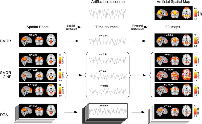
Experiment 1: Example of decreased FC map quality after including two (SMDR + 2 NR) or all (DRA) NR in dual regression. The time courses for two NR used in DRA for a subject correlated highly with the artificial time course; and the addition of the corresponding spatial prior regressors to SMDR reduced the CC quality score from 0.90 to 0.31. Portions of the artificial spatial map (showing where artificial signal was added) appeared to be contained within the FC MONI. Inclusion of all NR further reduced CC (0.24). Arrows represent regression, spatial or temporal, onto the session's fMRI data. Pearson correlation coefficients (r) show correlations with the top spatial map or time course in each column: SP MOI, artificial time course, or the artificial spatial map. Spatial maps were visualized with lower thresholds set (a) for spatial priors, with group ICA (FSL MELODIC) alternative hypothesis test at p > .95; (b) for the artificial spatial map, at 1/10 of maximum artificial signal amplitude; and (c) for the FC maps, at a z‐score where # false positive = # false negative voxels, defining true “activation” with the binary map that had been spatially blurred to create the artificial spatial map. All shown sagittal, coronal, and axial brain slices intersect at MNI coordinates [3, −63, 15]. FC, functional connectivity; FC MONI, FC maps of no interest; ICA, independent component analysis; MELODIC, Multivariate Exploratory Linear Decomposition into Independent Components; MNI, Montreal Neurological Institute; NR, nuisance regressors; SMDR, single‐map dual regression; SP MOI, spatial prior map of interest [Color figure can be viewed at http://wileyonlinelibrary.com]

Figure 7.

Experiment 3: Example of decreased FC map quality scores after including one (SMDR + 1 NR) or all (DRA) NR in dual regression. The time course for a nuisance regressor used in DRA, presumed to model structured noise (prominent activation in the sagittal sinus), correlated highly with the a priori time course; and the addition of the corresponding spatial prior regressor to SMDR reduced the CC quality score from 0.91 to 0.70. Portions of the thresholded SOC map appeared to be contained within the FC MONI. Inclusion of all NR further reduced CC (0.61). Arrows represent regression, spatial or temporal, onto the session's fMRI data. Pearson correlation coefficients (r) show correlations with the top spatial map or time course in each column: SP MOI, a priori time course, or SOC map. Spatial maps were visualized with lower thresholds set 1) for spatial priors, at a conventional threshold (z = 3.1); 2) for the SOC map, using FDR (false discovery rate); and 3) for the FC maps, at a z‐score where # false positive = # false negative voxels, using the thresholded SOC map to define true “activation.” All shown sagittal, coronal, and axial brain slices intersect at MNI coordinates [2, −26, −20]. FC, functional connectivity; FC MONI, FC maps of no interest; MNI, Montreal Neurological Institute; NR, nuisance regressors; SMDR, single‐map dual regression; SP MOI, spatial prior map of interest; SOC, standard‐of‐comparison [Color figure can be viewed at http://wileyonlinelibrary.com]

4. RESULTS

4.1. Independent component analysis

For Experiments 1 and 2, 30–55 components were derived from each single‐subject ICA prior to replacement of the natural DM components with artificial ones; and after replacement, 29–56 components were derived for Experiment 1 and 28–57 for Experiment 2. The group ICA (PICA) used for both experiments yielded 32 components. For Experiment 3, the number of group ICA (Infomax) components selected for each of the four runs varied from 7 to 18, within the range from the Laplace to Minimum Description Length (MDL) dimensionality estimates (Table 1); and correlations between each run's group task‐related GLM map and its MOI from group ICA ranged from 0.59 to 0.66.

Table 1.

Chosen dimensionality for Infomax group ICA, for each of the four runs in Experiment 3, compared with Laplace and Minimum Description Length (MDL) estimates. The rightmost column shows the correlation (r _MOI) between each run's map of interest (the group‐ICA map that represents the network of interest) and the run's group task‐related GLM map

Hand	Run sequence	Chosen dimensionality	Laplace estimate	MDL estimate	r MOI
Right	1	8	7	18	0.66
Right	2	8	6	17	0.66
Left	1	7	7	18	0.60
Left	2	18	6	18	0.59

Abbreviations: GLM, general linear model; ICA, independent component analysis; MOI, map of interest.

4.2. FC map accuracy

SMDR produced significantly more accurate FC maps compared with DRA (Figure 8), supporting our primary hypotheses. The decrease in DRA performance relative to SMDR was strongly associated with increased collinearity (z(R[T _ai,T _n]) or z(R[T _ap,T _n])) between the artificial (Experiment 1 and 2) or a priori (Experiment 3) time course and temporal NR (Figure 9). In turn, increased z(R[T _ai,T _n]) correlated significantly (r = .875, p < .001 for Experiment 1; and r = .869, p < .001 for Experiment 2) with increased spatial collinearity between SOCs and nuisance spatial priors (z(R[S _i,S _n])). Mean z(R[T _ai,T _n]) was significantly greater (p < .001) than mean z(R[T _ai,T _c]) in Experiment 1 (2.297 vs. 0.697) and Experiment 2 (2.338 vs. 1.178); and R(T _ai,T _n) was numerically greater than R(T _ai,T _c) for each of the 45 subjects in Experiment 1 (range 0.837–0.998 vs. 0.384–0.757) and for 44 subjects in Experiment 2 (range 0.876–0.998 vs. 0.758–0.888).

Figure 8.

Mean functional connectivity (FC) map quality scores, z(CC), where CC is the correlation between FC maps and SOC maps, for standard dual regression (DRA), and SMDR, for Experiments 1 and 2 and the four runs from Experiment 3. Key: *p < .05. **p < .01, ***p < .001; two‐tailed paired t tests, not corrected for multiple comparisons. FC, functional connectivity; SMDR, single‐map dual regression; SOC, standard‐of‐comparison

Figure 9.

Relationships between Fisher r‐to‐z transformed FC map quality scores, z(CC), and coefficients of multiple correlation with NR for artificial signal time course in Experiments 1 and 2, z(R[T _ai,T _n]), or a priori time course in Experiment 3, z(R[T _ap,T _n]). Higher z(R[T _ai,T _n]) and z(R[T _ap,T _n]) were significantly associated with lower z(CC) scores for standard dual regression with all spatial priors (DRA, second row), but not for SMDR (top row), resulting in significantly larger differences in quality scores (bottom row), z(CC_SMDR)–z(CC_DRA), with increasing collinearity between signal of interest (artificial or a priori time course) and NR. Upper left corners of scatter plots show correlations between z(CC) and z(R[T _ai,T _n]) or z(R[T _ap,T _n]), tested for statistical significance (uncorrected for multiple comparisons) with two‐tailed t tests against the null hypothesis of r = 0. FC, functional connectivity; NR, nuisance regressors; SMDR, single‐map dual regression

4.3. Denoising effects

In Experiments 1 and 2, FC map quality scores decreased for DRA, but increased for SMDR after denoising by regressing out selected (VIID) or all non‐DM IC time courses (Figure 10). The choice of full regression in preprocessing versus partial regression by adding regressors in the temporal regression step of DRA had little impact on quality scores (even though peak z‐scores and FC map SD differed in some cases, not shown); and consistent with theory, compared with standard DRA, DRA performed via step‐wise partial regression (pDRA, right‐most bar in left column of Figure 10) resulted in dramatically increased z‐scores (e.g., mean peak z‐score 22.5 in Experiment 1, compared with 12.9 for DRA), decreased ratio of peak z‐scores to z‐score SD (mean ratio 4.36 in Experiment 1, compared with 6.52 for DRA), slightly decreased CC scores, and no effect on PD scores (which were identical for all 45 subjects in both experiments).

Figure 10.

Mean FC map quality scores (z[CC] top two rows; PD bottom two rows), for Experiment 1 (Rows 1 and 3) and Experiment 2 (Rows 2 and 4), before and after denoising by regressing out temporal regressors derived from ICA, selected with visual inspection (VIID) or selected from the complete set of single‐subject ICs except for the default mode IC (non‐DM). Quality scores decreased with denoising for DRA (left column), but increased for SMDR (right column). The choice of full regression (in preprocessing) versus partial regression (in the temporal regression step of dual regression) had little effect on quality scores, even in comparing DRA with DRA variants where DRA's temporal NR were fully or partially regressed out in preprocessing (pre‐DRA, left column, rightmost pair of bars). Differences shown between results from full regression (black bars) and partial regression (adjacent gray bars) as well as between full regression and index comparator (left‐most gray bar in each bar chart) were statistically significant with p < .001 (uncorrected for multiple comparisons) in two‐tailed paired t tests (top two rows) or two‐tailed Wilcoxon's signed‐rank tests (bottom two rows). FC, functional connectivity; ICA, independent component analysis

Denoising via fICA, full regression using temporal regressors from single‐subject ICA, increased mean t _SNR (relative strength of the artificial signal of interest in regions where artificial signal had been added) for 15/45 cases in Experiment 1, and for no cases in Experiment 2; and denoising via pDRA increased mean t _SNR for 11/45 cases in Experiments 1 and 2 (Figure 11). On average, mean t _SNR decreased for both denoising methods in both experiments. The dispersion around mean values, CV(t _SNR), decreased for fICA, but increased markedly for pDRA in both experiments, and this increase was accompanied by a marked increase in the percentage of voxels that became anticorrelated with the artificial signal of interest, Pneg(t _SNR). In contrast, after fICA no anticorrelated voxels were found, except for a single voxel for one subject in Experiment 2.

Figure 11.

Artificial signal‐strength statistics, averaged over subjects in Experiment 1 (left column) and Experiment 2 (right column), in regions where artificial signal was added to synthetic fMRI data. Our measure of signal strength for the time course of a given voxel is t _SNR = r*sqrt(df/[1‐r ²]), where df is degrees of freedom for t‐score (=n−2, where n is the number of time points) and r is Pearson's correlation coefficient between the artificial signal and the voxel's time course. t _SNR is related to the signal‐to‐noise ratio, SNR = (signal variance)/(noise variance) = t _SNR ²/df. Shown for t _SNR are mean (mean[t _SNR], top row), coefficient of variation (CV[t _SNR], middle row), and percentage of negative voxels (Pneg[t _SNR], bottom row), before (none, left‐most bar in each chart) and after denoising by fully regressing out temporal regressors from components derived with ICA (fICA, middle bars) or by partially regressing out DRA's temporal nuisance regressors (pDRA, right‐most bars). fICA lowered voxels' mean artificial signal strength, mean(t _SNR), but could nonetheless improve detection of FC by reducing dispersion of voxel signal strength (CV[t _SNR]) around its mean, thereby improving detection for voxels whose signal strength would otherwise fall below thresholds for detection. In contrast, pDRA increased CV(t _SNR), thereby lowering signal strength for some voxels below thresholds for detection of FC, even to the point where voxel time courses became anticorrelated with the artificial signal of interest, as reflected in Pneg(t _SNR). Results after denoising within each bar graph differed significantly (p < .001) from those before denoising in two‐tailed Wilcoxon's signed‐rank tests. ICA, independent component analysis

4.4. Illustrative examples

Figure 6 illustrates a case where a subject's highly correlated temporal NR were associated with reduced quality of the FC map derived with DRA and SMDR + 2NR: The distribution map for signal of interest (SOC, Figure 6, upper right corner) was relatively highly correlated with two of the nuisance spatial priors (r = .52 and .36, compared with .38 for the spatial prior MOI; spatial priors shown in Figure 6, left column, labeled SMDR + 2NR), and after spatial regression the artificial signal of interest was highly correlated with the nuisance time courses corresponding to the nuisance spatial priors. After temporal regression, the corresponding nuisance FC maps (which resembled their corresponding spatial priors) contained regions of high FC in locations where the artificial signal should have been represented in the FC MOI for DRA and SMDR + 2NR (e.g., medial frontal), worsening the accuracy of the FC map. In contrast, Figure 7 shows a case where DRA may have improved FC map accuracy by removing FC that appears to represent structured noise (prominent in the sagittal sinus) whose signal was temporally correlated with the signal of interest. A bias in our SOC may explain why the quality score did not reflect this improvement: The structured noise was prominently represented in the SOC.

5. DISCUSSION

Our results suggest that inclusion of temporal NR in standard dual regression can worsen accuracy of derived FC maps, because of poor correspondence between the distribution of signal of interest within fMRI data and nuisance spatial priors included in the spatial regression step. This view is supported by theoretical arguments and empirical results from three experiments that demonstrate how FC maps derived from dual regression may in some, if not most, cases be enhanced by omitting NR. In particular, omission of NR may be necessary to allow enhancement of FC map quality with denoising procedures that remove structured noise from fMRI data (Figure 10).

In all three experiments, the accuracy of derived FC maps (z[CC]) was significantly lower for DRA compared with SMDR, and this decrease was significantly associated with increased collinearity between signal of interest and temporal NR used for DRA (R[T _ai,T _n] for Experiments 1 and 2; and R(T _ap,T _n) for Experiment 3). In Experiments 1 and 2, this increased collinearity was significantly associated with increased collinearity between the spatial distribution of signal of interest and nuisance spatial priors (R[S _i,S _n]), which supports the hypothesis that “misalignments” between the spatial distribution of signal of interest and nuisance spatial priors spawned spurious increases in collinearity between signal of interest and temporal NR derived via spatial regression. Further support is found in the remarkably high collinearity between signal of interest and temporal NR derived with DRA (R[T _ai,T _n]), compared with collinearity between the signal of interest and time courses derived from fMRI data with ICA (R[T _ai,T _c]).

The difference in FC map accuracy between DRA and SMDR was not merely a consequence of including temporal NR that correlate with the signal of interest. DRA performed via step‐wise partial regression (pDRA) eliminated the increase in variance of parameter estimates due to the inclusion of temporal NR, yielding FC maps with much higher peak z‐scores and z‐score SD, but no improvement in quality scores (Figure 10, left column, right‐most bar). In contrast, performing SMDR after regressing out sets of 30–55 temporally correlated (due to chance) NR (fICA) resulted in a marked improvement in FC map quality scores (Figure 10), even when the signal of interest was modified to make it highly correlated with one of those NR (Figure 10, Experiment 2). Although pDRA for some subjects and for many voxels was an effective denoising technique that increased the strength of the signal of interest relative to noise, t _SNR, this increase was accompanied by dramatic decreases in t _SNR for other voxels (Figures 3 and 11), causing them to fall below detection thresholds in FC maps, resulting in low PD scores; and the heterogeneity in voxel t _SNR values (Figure 11, middle row) also distorted the “shape” of the distribution of t _SNR relative to the nearly uniform distribution of artificial signal of interest that had been added to create the synthetic fMRI data, resulting in low CC scores. In contrast, and especially for Experiment 2, fICA caused a global reduction in t _SNR that simultaneously reduced the dispersion of t _SNR values, resulting in improved detection and preservation of the shape of the distribution of added signal of interest.

The loss in accuracy of DRA compared with SMDR in Experiments 1 and 2 may have been exacerbated by the apparent split of the DM into three spatial priors, each of which resembled the DM. The split in the DM component limited the quality of the selected DM spatial prior, which negatively impacted the accuracy of FC maps derived from this spatial prior with dual regression. However, even after repeating Experiment 1 with variants where the number of components for group ICA and/or individual‐subject ICA were limited (resulting in only a single DM spatial prior rather than three upon visual inspection), and with an improved, nonlinear registration technique (FSL FNIRT), DRA still performed poorly compared with SMDR (Appendix A). Furthermore, SMDR seemed more resilient than DRA in detecting functional activation corresponding to portions of individual‐subject artificial DM spatial maps that were not represented in the spatial prior of interest (Figure 6). Some individual variability might be lost with DRA by forcing the FC maps from individual subjects to “conform” to group‐level spatial priors, as suggested by Gordon, Stollstorff, and Vaidya (2012) and supported by our findings: Compared with SMDR, FC maps derived with DRA correlated more highly with their corresponding spatial priors (Appendix B), but less highly with their corresponding SOCs. This potential bias with DRA can be particularly problematic because unless the spatial prior of interest precisely represents the full extent of the network of interest for all subjects, portions of individual‐subject FC maps may be suppressed.

Another potential limitation of DRA is that it can prevent regression‐based and other denoising techniques from improving FC map quality (Figure 10), because their use can further exacerbate spurious collinearity between signal of interest and temporal NR (Figure 2, Case C). Removing from fMRI data, a signal that corresponds to a nuisance spatial prior creates a vacuum of signal within its spatial map, allowing other signals to represent the spatial prior after spatial regression. This process markedly reduces FC map accuracy when the signal of interest represents that spatial prior in the corresponding temporal nuisance regressor. DRA provides group ICA‐based denoising but is insufficient to replace standard regression‐based denoising techniques. Many noise sources cannot be removed from fMRI data with group ICA‐based denoising because they are not consistent across subjects (Wang & Peterson, 2008) or sessions (Zuo et al., 2010); and larger, more stable components can often be removed by other denoising techniques. For example, group ICA commonly shows a component representing brain white matter (Biswal et al., 2010; Kelly et al., 2010; Smith et al., 2009), but regressing out white‐matter signal with DRA is unnecessary because the white‐matter signal can be removed by regressing out the average time course from white matter (Birn, 2012). Finally, denoising by eliminating noise components identified from individual‐subject ICA is preferable to denoising via group ICA because the denoising is tailored to each subject's functional anatomy. After denoising by removal of noise components identified with visual inspection of individual‐subject ICs, few (Griffanti et al., 2017), if any (Kelly et al., 2010), noise components would be expected among group ICs. Such denoising can also be performed automatically with, for example, ICA‐AROMA (Pruim, Mennes, van Rooij, et al., 2015; Pruim, Mennes, Buitelaar, & Beckmann, 2015).

Dual regression can be a powerful tool for determination of FC, provided that pitfalls outlined in this article are avoided. Omission of NR in the derivation of FC maps from dual regression can prevent a potential source of error whose impact cannot be gauged precisely without knowledge of the exact spatial distributions of signals within the fMRI data. Rather than include all spatial maps from group ICA as spatial priors (Abram et al., 2017; Filippini et al., 2009; Geissmann et al., 2018; Muetzel et al., 2016; Pannekoek et al., 2015; Rueter, Abram, MacDonald, Rustichini, & DeYoung, 2018; Smith et al., 2015), some dual regression studies omit spatial priors thought to represent noise (Baggio et al., 2015; Fan et al., 2017; Giorgio, Zhang, Costantino, De Stefano, & Frezzotti, 2018; Ishaque et al., 2017; Klaassens et al., 2017; Schumacher et al., 2018); however, the remaining “nuisance” spatial maps may still reduce FC map accuracy, through mechanisms described in this article: Appendix A shows an example where DRA quality scores did not improve after omitting only spatial priors thought to represent structured noise. Reduction of NR to a small number that are highly consistent in spatial distributions across all subjects/sessions might avoid these pitfalls, provided that denoising procedures do not remove the signal corresponding to these NR from the fMRI data. For example, if a nuisance spatial prior representing white matter is included in dual regression, as in Biswal et al. (2010), then, regressing out white matter signal in preprocessing should be avoided. Including multiple spatial priors of interest in dual regression may be useful in cases where the corresponding signal sources are expected to be highly collinear, to parse the variance contributed by each signal source separately (Leech et al., 2011). However, unless the spatial distributions of these signals can be presumed to be extremely consistent across subjects/sessions, the potential bias of derived FC maps toward “conforming” to the spatial prior maps should be considered in the interpretation of results. Appendix C provides metrics to assist with weighing risks versus benefits of including NR in dual regression.

In light of our current findings, it may be useful to reassess and/or replicate prior studies, to include SMDR as a comparator, when DRA is compared to other methods for deriving FC. For example, Smith et al. (2014) demonstrated better performance for DRA in deriving FC, compared with a variant of SCA that included DRA's NR, but both methods might improve in performance by omitting DRA's NR; and they might further improve by including NR that represent global signal or signal from white matter and cerebrospinal fluid, as is common practice for SCA (Birn, 2012). Replication to include SMDR in place of DRA might also be considered for a study by Erhardt, Rachakonda, et al. (2011) that compared methods for “back reconstruction” of individual‐subject spatial maps from a set of spatial priors, finding better performance for GICA3 compared with DRA. Perhaps a new variant of GICA, analogous to SMDR, might provide more accurate FC maps and greater resilience to deleterious effects of spatial misalignments between spatial priors and corresponding individual‐subject spatial distributions of signal; but our theoretical and empirical findings do not lend themselves easily to such an extrapolation.

Limitations of our study include the use of natural data in Experiment 3, with a priori time courses representing signal of interest, which might have biased FC map quality scores in favor of SMDR. Noise‐related activity that correlated with the a priori time course might have been suppressed in DRA‐derived FC maps of interest, decreasing their correlations with the SOCs (Figure 6): SMDR produced FC maps more closely matching those from task‐fMRI, but not necessarily better in quality overall. Conversely, the use of SOCs derived from single‐subject ICA in Experiments 1 and 2 might have biased FC map quality scores in favor of DRA. The inclusion, in SMDR‐derived DM maps, of FC from non‐DM components that are correlated with the DM component would tend to lower quality scores for SMDR, even if such FC could be considered part of a more encompassing DM network. We reduced the impact of this bias by limiting the number (0 or 1) of non‐DM components that were highly correlated with the signal of interest. In Experiments 1 and 2, the simple, well‐characterized artificial signal facilitated tasks of visual inspection and illustration but did not simulate some properties of neural signals in fMRI data: It had no time lag among voxels relative to each other, and was uniform in intensity with a sharp decrease at borders of ICA‐derived brain regions that may not have adequately modeled spatial distributions of DM activity. We partially addressed limitations by exploring four additional variants of Experiment 1 (Appendix D), finding again superior performance for SMDR over DRA that was related to collinearity between signal of interest and temporal NR; but it is not clear how to generalize from these results to the full spectrum of natural fMRI experiments.

A comprehensive assessment of which NR to exclude from standard dual regression and under what circumstances is beyond the scope of this article. However, SMDR provides a simple alternative, akin to SFCs (Kelly et al., 2010), that does not risk inadvertently regressing out signal of interest. Effective denoising can be added to SMDR with temporal NR that model noise, such as those derived from single‐subject ICA (Griffanti et al., 2014; Kelly et al., 2010; Kelly, Alexopoulos, Gunning, & Hoptman, 2017; Pruim, Mennes, Buitelaar, & Beckmann, 2015; Pruim, Mennes, van Rooij, et al., 2015; Salimi‐Khorshidi et al., 2014) or related to subject motion (Birn, 2012; Satterthwaite et al., 2013; Van Dijk et al., 2010; Yan et al., 2013). Denoising by aggressively filtering out nearly all single‐subject IC time courses was highly effective in Experiments 1 and 2, where there was no risk of regressing out the artificial signal of interest; but in practice, caution is advised to avoid inadvertently regressing out the time course for an IC that closely represents the signal of interest (Kelly et al., 2017).

6. CONCLUSION

High temporal correlations between signal of interest and NR in standard dual regression can complicate the interpretation of derived FC maps and compromise their accuracy. SMDR offers a viable alternative, whose FC maps may be more easily interpreted and, in some cases, more accurate than those derived with standard dual regression.

CONFLICT OF INTEREST

The authors declare no competing conflict of interest.

Supporting information

Appendix S1: APPENDICES

Figure A1 Mean functional connectivity map quality scores (z[CC]) in four variants of Experiment 1, comparing standard dual regression (DRA) and single‐map dual regression (SMDR). CC is the correlation between functional connectivity maps and standard‐of‐comparison maps. Variant 1: Spatial priors were derived from our synthetic data with group ICA dimensionality = 20. Variant 2: Spatial priors were downloaded from publicly available resting‐state components derived with group ICA dimensionality = 20. Variants 3 and 4: Variants 1 and 2 repeated using synthetic data derived with non‐linear registration (FSL FNIRT) and dimensionality = 20 for individual‐subject ICAs. Differences shown within pairs of results were statistically significant (p < 0.001) using two‐tailed paired t‐tests, not corrected for multiple comparisons.

Figure B1 Mean z(r _sp) spatial correlations between spatial priors of interest and corresponding functional connectivity maps used for standard dual regression (DRA) and single‐map dual regression (SMDR), for Experiments 1–2 and the four runs from Experiment 3. Key: ** – p < 0.01, *** – p < 0.001; two‐tailed paired t‐tests, not corrected for multiple comparisons.

Figure C1 Metrics z(R _dn) (left column) and z(R _dn) – z(R _dc) (right column) as predictors of difference in quality scores between SMDR and DRA (z(CC_SMDR) – z(CC_DRA)) for modified Experiments 1 (top row) and 2 (bottom row). R _dn is the coefficient of multiple correlation for derived signal of interest with DRA's temporal nuisance regressors, and R _dc is the coefficient of multiple correlation for derived signal of interest with non‐DM signal sources derived from single‐subject ICA. Upper left corners of scatter plots show correlations between z(CC_SMDR) – z(CC_DRA) and each metric, tested for statistical significance (uncorrected for multiple comparisons) with two‐tailed t‐tests against the null hypothesis of r = 0.

Figure D1 Additional variants of Experiment 1, using realistic artificial time course and spatial maps, with an alternative method for identifying the default‐mode component. Shown are mean functional connectivity map quality scores (z[CC]) for standard dual regression (DRA) and single‐map dual regression (SMDR), before (DRA and SMDR) and after (D + DRA and D + SMDR) aggressive denoising by fully regressing out all non‐default‐mode components, using spatial priors from group ICA before (Original ICs) and after (Z‐score Maps) voxel‐wise conversion of ICs to z‐score maps. Pair‐wise differences in results shown within each group of spatial priors were all statistically significant (p < 0.001) using two‐tailed paired t‐tests, not corrected for multiple comparisons. Pair‐wise differences across groups for each method were also statistically significant (p < 0.001), except for D + SMDR (p = 0.19).

Kelly RE Jr., Hoptman MJ, Alexopoulos GS, Gunning FM, McKeown MJ. Omission of temporal nuisance regressors from dual regression can improve accuracy of fMRI functional connectivity maps. Hum Brain Mapp. 2019;40:4005–4025. 10.1002/hbm.24692

REFERENCES

- Abbott, C. , Il, K. D. , Bustillo, J. , & Calhoun, V. (2010). Decreased modulation of the anterior default mode network during novelty detection in older patients with schizophrenia. The American Journal of Geriatric Psychiatry, 18, S93–S94. [DOI] [PMC free article] [PubMed] [Google Scholar]
- Abram, S. V. , Wisner, K. M. , Fox, J. M. , Barch, D. M. , Wang, L. , Csernansky, J. G. , … Smith, M. J. (2017). Fronto‐temporal connectivity predicts cognitive empathy deficits and experiential negative symptoms in schizophrenia. Human Brain Mapping, 38, 1111–1124. [DOI] [PMC free article] [PubMed] [Google Scholar]
- Aguirre, G. K. , Zarahn, E. , & D'Esposito, M. (1998). The inferential impact of global signal covariates in functional neuroimaging analyses. NeuroImage, 8, 302–306. [DOI] [PubMed] [Google Scholar]
- Ardekani, B. A. , Guckemus, S. , Bachman, A. , Hoptman, M. J. , Wojtaszek, M. , & Nierenberg, J. (2005). Quantitative comparison of algorithms for inter‐subject registration of 3D volumetric brain MRI scans. Journal of Neuroscience Methods, 142, 67–76. [DOI] [PubMed] [Google Scholar]
- Baggio, H. C. , Segura, B. , Sala‐Llonch, R. , Marti, M. J. , Valldeoriola, F. , Compta, Y. , … Junqué, C. (2015). Cognitive impairment and resting‐state network connectivity in Parkinson's disease. Human Brain Mapping, 36, 199–212. [DOI] [PMC free article] [PubMed] [Google Scholar]
- Bartels, A. , & Zeki, S. (2005). Brain dynamics during natural viewing conditions—A new guide for mapping connectivity in vivo. NeuroImage, 24, 339–349. [DOI] [PubMed] [Google Scholar]
- Beckmann, C. F. (2012). Modelling with independent components. NeuroImage, 62, 891–901. [DOI] [PubMed] [Google Scholar]
- Beckmann, C. F. , DeLuca, M. , Devlin, J. T. , & Smith, S. M. (2005). Investigations into resting‐state connectivity using independent component analysis. Philosophical Transactions of the Royal Society of London. Series B, Biological Sciences, 360, 1001–1013. [DOI] [PMC free article] [PubMed] [Google Scholar]
- Beckmann, C.F. , Mackay, C.E. , Filippini, N. , & Smith, S.M. (2009): Group comparison of resting‐state FMRI data using multi‐subject ICA and dual regression. 15th Annual Meeting of Organization for Human Brain Mapping, poster 441 SU‐AM.
- Beckmann, C. F. , & Smith, S. M. (2004). Probabilistic independent component analysis for functional magnetic resonance imaging. IEEE Transactions on Medical Imaging, 23, 137–152. [DOI] [PubMed] [Google Scholar]
- Beckmann, C. F. , & Smith, S. M. (2005). Tensorial extensions of independent component analysis for multisubject FMRI analysis. NeuroImage, 25, 294–311. [DOI] [PubMed] [Google Scholar]
- Bell, A. J. , & Sejnowski, T. J. (1995). An information‐maximization approach to blind separation and blind deconvolution. Neural Computation, 7, 1129–1159. [DOI] [PubMed] [Google Scholar]
- Birn, R. M. (2012). The role of physiological noise in resting‐state functional connectivity. NeuroImage, 62(2), 864–870. [DOI] [PubMed] [Google Scholar]
- Birn, R. M. , Murphy, K. , & Bandettini, P. A. (2008). The effect of respiration variations on independent component analysis results of resting state functional connectivity. Human Brain Mapping, 29, 740–750. [DOI] [PMC free article] [PubMed] [Google Scholar]
- Birn, R. M. , Murphy, K. , Handwerker, D. A. , & Bandettini, P. A. (2009). fMRI in the presence of task‐correlated breathing variations. NeuroImage, 47, 1092–1104. [DOI] [PMC free article] [PubMed] [Google Scholar]
- Biswal, B. , Yetkin, F. Z. , Haughton, V. M. , & Hyde, J. S. (1995). Functional connectivity in the motor cortex of resting human brain using echo‐planar MRI. Magnetic Resonance in Medicine, 34, 537–541. [DOI] [PubMed] [Google Scholar]
- Biswal, B. B. , Mennes, M. , Zuo, X. N. , Gohel, S. , Kelly, C. , Smith, S. M. , … Milham, M. P. (2010). Toward discovery science of human brain function. Proceedings of the National Academy of Sciences of the United States of America, 107, 4734–4739. [DOI] [PMC free article] [PubMed] [Google Scholar]
- Bright, M. G. , Tench, C. R. , & Murphy, K. (2017). Potential pitfalls when denoising resting state fMRI data using nuisance regression. NeuroImage, 154, 159–168. [DOI] [PMC free article] [PubMed] [Google Scholar]
- Caballero‐Gaudes, C. , & Reynolds, R. C. (2017). Methods for cleaning the BOLD fMRI signal. NeuroImage, 154, 128–149. [DOI] [PMC free article] [PubMed] [Google Scholar]
- Calhoun, V. D. , Adali, T. , McGinty, V. B. , Pekar, J. J. , Watson, T. D. , & Pearlson, G. D. (2001). fMRI activation in a visual‐perception task: Network of areas detected using the general linear model and independent components analysis. NeuroImage, 14, 1080–1088. [DOI] [PubMed] [Google Scholar]
- Calhoun, V. D. , Adali, T. , Pearlson, G. D. , & Pekar, J. J. (2001). A method for making group inferences from functional MRI data using independent component analysis. Human Brain Mapping, 14, 140–151. [DOI] [PMC free article] [PubMed] [Google Scholar]
- Calhoun, V. D. , Adali, T. , Stevens, M. C. , Kiehl, K. A. , & Pekar, J. J. (2005). Semi‐blind ICA of fMRI: A method for utilizing hypothesis‐derived time courses in a spatial ICA analysis. NeuroImage, 25, 527–538. [DOI] [PubMed] [Google Scholar]
- Calhoun, V. D. , Kiehl, K. A. , Liddle, P. F. , & Pearlson, G. D. (2004). Aberrant localization of synchronous hemodynamic activity in auditory cortex reliably characterizes schizophrenia. Biological Psychiatry, 55, 842–849. [DOI] [PMC free article] [PubMed] [Google Scholar]
- Calhoun, V. D. , Liu, J. , & Adali, T. (2009). A review of group ICA for fMRI data and ICA for joint inference of imaging, genetic, and ERP data. NeuroImage, 45, S163–S172. [DOI] [PMC free article] [PubMed] [Google Scholar]
- Cardinale, R. C. , Shih, P. , Fishman, I. , Ford, L. M. , & Muller, R. A. (2013). Pervasive rightward asymmetry shifts of functional networks in autism spectrum disorder. JAMA Psychiatry, 70, 975–982. [DOI] [PMC free article] [PubMed] [Google Scholar]
- Chahine, G. , Richter, A. , Wolter, S. , Goya‐Maldonado, R. , & Gruber, O. (2017). Disruptions in the left frontoparietal network underlie resting state endophenotypic markers in schizophrenia. Human Brain Mapping, 38, 1741–1750. [DOI] [PMC free article] [PubMed] [Google Scholar]
- Chen, G. , Xie, C. , Ward, B. D. , Li, W. , Antuono, P. , & Li, S. J. (2012). A method to determine the necessity for global signal regression in resting‐state fMRI studies. Magnetic Resonance in Medicine, 68, 1828–1835. [DOI] [PMC free article] [PubMed] [Google Scholar]
- Ciric, R. , Wolf, D. H. , Power, J. D. , Roalf, D. R. , Baum, G. L. , Ruparel, K. , … Satterthwaite, T. D. (2017). Benchmarking of participant‐level confound regression strategies for the control of motion artifact in studies of functional connectivity. NeuroImage, 154, 174–187. [DOI] [PMC free article] [PubMed] [Google Scholar]
- Correa, N. , Adali, T. , & Calhoun, V. D. (2007). Performance of blind source separation algorithms for fMRI analysis using a group ICA method. Magnetic Resonance Imaging, 25, 684–694. [DOI] [PMC free article] [PubMed] [Google Scholar]
- Davey, C. E. , Grayden, D. B. , Egan, G. F. , & Johnston, L. A. (2013). Filtering induces correlation in fMRI resting state data. NeuroImage, 64, 728–740. [DOI] [PubMed] [Google Scholar]
- Duncan, K. J. , Pattamadilok, C. , Knierim, I. , & Devlin, J. T. (2009). Consistency and variability in functional localisers. NeuroImage, 46, 1018–1026. [DOI] [PMC free article] [PubMed] [Google Scholar]
- Erhardt, E. B. , Allen, E. A. , Damaraju, E. , & Calhoun, V. D. (2011). On network derivation, classification, and visualization: A response to Habeck and Moeller. Brain Connectivity, 1, 105–110. [DOI] [PMC free article] [PubMed] [Google Scholar]
- Erhardt, E. B. , Rachakonda, S. , Bedrick, E. J. , Allen, E. A. , Adali, T. , & Calhoun, V. D. (2011). Comparison of multi‐subject ICA methods for analysis of fMRI data. Human Brain Mapping, 32, 2075–2095. [DOI] [PMC free article] [PubMed] [Google Scholar]
- Fan, J. , Taylor, P. A. , Jacobson, S. W. , Molteno, C. D. , Gohel, S. , Biswal, B. B. , … Meintjes, E. M. (2017). Localized reductions in resting‐state functional connectivity in children with prenatal alcohol exposure. Human Brain Mapping, 38, 5217–5233. [DOI] [PMC free article] [PubMed] [Google Scholar]
- Filippini, N. , MacIntosh, B. J. , Hough, M. G. , Goodwin, G. M. , Frisoni, G. B. , Smith, S. M. , … Mackay, C. E. (2009). Distinct patterns of brain activity in young carriers of the APOE‐epsilon4 allele. Proceedings of the National Academy of Sciences of the United States of America, 106, 7209–7214. [DOI] [PMC free article] [PubMed] [Google Scholar]
- Fox, M. D. , Snyder, A. Z. , Vincent, J. L. , Corbetta, M. , Van Essen, D. C. , & Raichle, M. E. (2005). The human brain is intrinsically organized into dynamic, anticorrelated functional networks. Proceedings of the National Academy of Sciences of the United States of America, 102, 9673–9678. [DOI] [PMC free article] [PubMed] [Google Scholar]
- Friston, K. (2002). Beyond phrenology: What can neuroimaging tell us about distributed circuitry? Annual Review of Neuroscience, 25, 221–250. [DOI] [PubMed] [Google Scholar]
- Friston, K. J. , Holmes, A. P. , Poline, J. B. , Grasby, P. J. , Williams, S. C. , Frackowiak, R. S. , & Turner, R. (1995). Analysis of fMRI time‐series revisited. NeuroImage, 2, 45–53. [DOI] [PubMed] [Google Scholar]
- Geissmann, L. , Gschwind, L. , Schicktanz, N. , Deuring, G. , Rosburg, T. , Schwegler, K. , … Coynel, D. (2018). Resting‐state functional connectivity remains unaffected by preceding exposure to aversive visual stimuli. NeuroImage, 167, 354–365. [DOI] [PubMed] [Google Scholar]
- Giorgio, A. , Zhang, J. , Costantino, F. , De Stefano, N. , & Frezzotti, P. (2018). Diffuse brain damage in normal tension glaucoma. Human Brain Mapping, 39, 532–541. [DOI] [PMC free article] [PubMed] [Google Scholar]
- Glass, G. V. , & Stanley, J. C. (1970). Statistical methods in education and psychology (Vol. 596). Englewood Cliffs, NJ: Prentice‐Hall. [Google Scholar]
- Glasser, M. F. , Sotiropoulos, S. N. , Wilson, J. A. , Coalson, T. S. , Fischl, B. , Andersson, J. L. , … Consortium WU‐MH . (2013). The minimal preprocessing pipelines for the human connectome project. NeuroImage, 80, 105–124. [DOI] [PMC free article] [PubMed] [Google Scholar]
- Glasser, M. F. C. , Coalson, T. S. , Robinson, E. C. , Hacker, C. D. , Harwell, J. , Yacoub, E. , … Van Essen, D. C. (2016). A multi‐modal parcellation of human cerebral cortex. Nature, 536, 171–178. [DOI] [PMC free article] [PubMed] [Google Scholar]
- Gordon, E. M. , Laumann, T. O. , Adeyemo, B. , Huckins, J. F. , Kelley, W. M. , & Petersen, S. E. (2016). Generation and evaluation of a cortical area parcellation from resting‐state correlations. Cerebral Cortex, 26, 288–303. [DOI] [PMC free article] [PubMed] [Google Scholar]
- Gordon, E. M. , Laumann, T. O. , Adeyemo, B. , & Petersen, S. E. (2017). Individual variability of the system‐level organization of the human brain. Cerebral Cortex, 27, 386–399. [DOI] [PMC free article] [PubMed] [Google Scholar]
- Gordon, E. M. , Stollstorff, M. , & Vaidya, C. J. (2012). Using spatial multiple regression to identify intrinsic connectivity networks involved in working memory performance. Human Brain Mapping, 33, 1536–1552. [DOI] [PMC free article] [PubMed] [Google Scholar]
- Gorgolewski, K. J. , Storkey, A. , Bastin, M. E. , Whittle, I. R. , Wardlaw, J. M. , & Pernet, C. R. (2013). A test‐retest fMRI dataset for motor, language and spatial attention functions. GigaScience, 2, 6. [DOI] [PMC free article] [PubMed] [Google Scholar]
- Greicius, M. D. , Flores, B. H. , Menon, V. , Glover, G. H. , Solvason, H. B. , Kenna, H. , … Schatzberg, A. F. (2007). Resting‐state functional connectivity in major depression: Abnormally increased contributions from subgenual cingulate cortex and thalamus. Biological Psychiatry, 62, 429–437. [DOI] [PMC free article] [PubMed] [Google Scholar]
- Greicius, M. D. , Srivastava, G. , Reiss, A. L. , & Menon, V. (2004). Default‐mode network activity distinguishes Alzheimer's disease from healthy aging: Evidence from functional MRI. Proceedings of the National Academy of Sciences of the United States of America, 101, 4637–4642. [DOI] [PMC free article] [PubMed] [Google Scholar]
- Griffanti, L. , Douaud, G. , Bijsterbosch, J. , Evangelisti, S. , Alfaro‐Almagro, F. , Glasser, M. F. , … Smith, S. M. (2017). Hand classification of fMRI ICA noise components. NeuroImage, 154, 188–205. [DOI] [PMC free article] [PubMed] [Google Scholar]
- Griffanti, L. , Salimi‐Khorshidi, G. , Beckmann, C. F. , Auerbach, E. J. , Douaud, G. , Sexton, C. E. , … Smith, S. M. (2014). ICA‐based artefact removal and accelerated fMRI acquisition for improved resting state network imaging. NeuroImage, 95, 232–247. [DOI] [PMC free article] [PubMed] [Google Scholar]
- Gu, H. , Engelien, W. , Feng, H. , Silbersweig, D. A. , Stern, E. , & Yang, Y. (2001). Mapping transient, randomly occurring neuropsychological events using independent component analysis. NeuroImage, 14, 1432–1443. [DOI] [PubMed] [Google Scholar]
- Haaland, K. Y. , Elsinger, C. L. , Mayer, A. R. , Durgerian, S. , & Rao, S. M. (2004). Motor sequence complexity and performing hand produce differential patterns of hemispheric lateralization. Journal of Cognitive Neuroscience, 16, 621–636. [DOI] [PubMed] [Google Scholar]
- Handwerker, D. A. , Ollinger, J. M. , & D'Esposito, M. (2004). Variation of BOLD hemodynamic responses across subjects and brain regions and their effects on statistical analyses. NeuroImage, 21, 1639–1651. [DOI] [PubMed] [Google Scholar]
- Huettel, S. A. , Song, A. W. , & McCarthy, G. (2014). Functional magnetic resonance imaging (p. 573). Sunderland, MA: Sinauer Associates. [Google Scholar]
- Hyvarinen, A. (1999). Fast and robust fixed‐point algorithms for independent component analysis. IEEE Transactions on Neural Networks, 10, 626–634. [DOI] [PubMed] [Google Scholar]
- Ishaque, M. , Manning, J. H. , Woolsey, M. D. , Franklin, C. G. , Tullis, E. W. , Beckmann, C. F. , & Fox, P. T. (2017). Functional integrity in children with anoxic brain injury from drowning. Human Brain Mapping, 38, 4813–4831. [DOI] [PMC free article] [PubMed] [Google Scholar]
- Jenkinson, M. , Bannister, P. , Brady, M. , & Smith, S. (2002). Improved optimization for the robust and accurate linear registration and motion correction of brain images. NeuroImage, 17, 825–841. [DOI] [PubMed] [Google Scholar]
- Jenkinson, M. , Beckmann, C. F. , Behrens, T. E. , Woolrich, M. W. , & Smith, S. M. (2012). FSL. NeuroImage, 62, 782–790. [DOI] [PubMed] [Google Scholar]
- Jenkinson, M. , & Smith, S. (2001). A global optimisation method for robust affine registration of brain images. Medical Image Analysis, 5, 143–156. [DOI] [PubMed] [Google Scholar]
- Kelly, R. E., Jr. , Alexopoulos, G. S. , Gunning, F. M. , & Hoptman, M. J. (2017). Advocating for well‐defined and validated procedures: Comment on Griffanti et al., Neuroimage 154:188‐205. Journal of Neuroscience Methods, 290, 24–26. [DOI] [PubMed] [Google Scholar]
- Kelly, R. E., Jr. , Alexopoulos, G. S. , Wang, Z. , Gunning, F. M. , Murphy, C. F. , Morimoto, S. S. , … Hoptman, M. J. (2010). Visual inspection of independent components: Defining a procedure for artifact removal from fMRI data. Journal of Neuroscience Methods, 189, 233–245. [DOI] [PMC free article] [PubMed] [Google Scholar]
- Kelly, R. E. , Wang, Z. , Alexopoulos, G. S. , Gunning, F. M. , Murphy, C. F. , Morimoto, S. S. , … Hoptman, M. J. (2010). Hybrid ICA‐seed‐based methods for fMRI functional connectivity assessment: A feasibility study. International Journal of Biomedical Imaging, 2010, 868976. [DOI] [PMC free article] [PubMed] [Google Scholar]
- Klaassens, B. L. , Rombouts, S. A. R. B. , Winkler, A. M. , van Gorsel, H. C. , van der Grond, J. , & van Gerven, J. M. A. (2017). Time related effects on functional brain connectivity after serotonergic and cholinergic neuromodulation. Human Brain Mapping, 38, 308–325. [DOI] [PMC free article] [PubMed] [Google Scholar]
- Klein, A. , Andersson, J. , Ardekani, B. A. , Ashburner, J. , Avants, B. , Chiang, M. C. , … Parsey, R. V. (2009). Evaluation of 14 nonlinear deformation algorithms applied to human brain MRI registration. NeuroImage, 46, 786–802. [DOI] [PMC free article] [PubMed] [Google Scholar]
- Laumann, T. O. , Gordon, E. M. , Adeyemo, B. , Snyder, A. Z. , Joo, S. J. , Chen, M. Y. , … Petersen, S. E. (2015). Functional system and areal organization of a highly sampled individual human brain. Neuron, 87, 657–670. [DOI] [PMC free article] [PubMed] [Google Scholar]
- Leech, R. , Kamourieh, S. , Beckmann, C. F. , & Sharp, D. J. (2011). Fractionating the default mode network: Distinct contributions of the ventral and dorsal posterior cingulate cortex to cognitive control. The Journal of Neuroscience, 31, 3217–3224. [DOI] [PMC free article] [PubMed] [Google Scholar]
- Lin, Q. H. , Liu, J. , Zheng, Y. R. , Liang, H. , & Calhoun, V. D. (2010). Semiblind spatial ICA of fMRI using spatial constraints. Human Brain Mapping, 31, 1076–1088. [DOI] [PMC free article] [PubMed] [Google Scholar]
- McKeown, M. J. (2000). Detection of consistently task‐related activations in fMRI data with hybrid independent component analysis. NeuroImage, 11, 24–35. [DOI] [PubMed] [Google Scholar]
- McKeown, M. J. , Hansen, L. K. , & Sejnowsk, T. J. (2003). Independent component analysis of functional MRI: What is signal and what is noise? Current Opinion in Neurobiology, 13, 620–629. [DOI] [PMC free article] [PubMed] [Google Scholar]
- McKeown, M. J. , Makeig, S. , Brown, G. G. , Jung, T. P. , Kindermann, S. S. , Bell, A. J. , & Sejnowski, T. J. (1998). Analysis of fMRI data by blind separation into independent spatial components. Human Brain Mapping, 6, 160–188. [DOI] [PMC free article] [PubMed] [Google Scholar]
- Minka, T.P. (2000). Automatic choice of dimensionality for PCA MIT Media Laboratory Vision and Modeling Group. Technical Report 514.
- Morey, R. A. , Petty, C. M. , Xu, Y. , Hayes, J. P. , Wagner, H. R., III , Lewis, D. V. , … McCarthy, G. (2009). A comparison of automated segmentation and manual tracing for quantifying hippocampal and amygdala volumes. NeuroImage, 45, 855–866. [DOI] [PMC free article] [PubMed] [Google Scholar]
- Mueller, S. , Wang, D. , Fox, M. D. , Yeo, B. T. , Sepulcre, J. , Sabuncu, M. R. , … Liu, H. (2013). Individual variability in functional connectivity architecture of the human brain. Neuron, 77, 586–595. [DOI] [PMC free article] [PubMed] [Google Scholar]
- Muetzel, R. L. , Blanken, L. M. E. , Thijssen, S. , van der Lugt, A. , Jaddoe, V. W. V. , Verhulst, F. C. , … White, T. (2016). Resting‐state networks in 6‐to‐10 year old children. Human Brain Mapping, 37, 4286–4300. [DOI] [PMC free article] [PubMed] [Google Scholar]
- Murphy, K. , Birn, R. M. , & Bandettini, P. A. (2013). Resting‐state fMRI confounds and cleanup. NeuroImage, 80, 349–359. [DOI] [PMC free article] [PubMed] [Google Scholar]
- Murphy, K. , Birn, R. M. , Handwerker, D. A. , Jones, T. B. , & Bandettini, P. A. (2009). The impact of global signal regression on resting state correlations: Are anti‐correlated networks introduced? NeuroImage, 44, 893–905. [DOI] [PMC free article] [PubMed] [Google Scholar]
- Murphy, K. , & Fox, M. D. (2017). Towards a consensus regarding global signal regression for resting state functional connectivity MRI. NeuroImage, 154, 169–173. [DOI] [PMC free article] [PubMed] [Google Scholar]
- Odish, O. F. F. , van den Berg‐Huysmans, A. A. , van den Bogaard, S. J. A. , Dumas, E. M. , Hart, E. P. , Rombouts, S. A. R. B. , … Roos, R. A. C. (2015). Longitudinal resting state fMRI analysis in healthy controls and premanifest Huntington's disease gene carriers: A three‐year follow‐up study. Human Brain Mapping, 36, 110–119. [DOI] [PMC free article] [PubMed] [Google Scholar]
- Pannekoek, J. N. , van der Werff, S. J. A. , van Tol, M. J. , Veltman, D. J. , Aleman, A. , Zitman, F. G. , … van der Wee, N. J. A. (2015). Investigating distinct and common abnormalities of resting‐state functional connectivity in depression, anxiety, and their comorbid states. European Neuropsychopharmacology, 25, 1933–1942. [DOI] [PubMed] [Google Scholar]
- Power, J. D. , Mitra, A. , Laumann, T. O. , Snyder, A. Z. , Schlaggar, B. L. , & Petersen, S. E. (2014). Methods to detect, characterize, and remove motion artifact in resting state fMRI. NeuroImage, 84, 320–341. [DOI] [PMC free article] [PubMed] [Google Scholar]
- Power, J. D. , Schlaggar, B. L. , & Petersen, S. E. (2015). Recent progress and outstanding issues in motion correction in resting state fMRI. NeuroImage, 105, 536–551. [DOI] [PMC free article] [PubMed] [Google Scholar]
- Pruim, R. H. , Mennes, M. , Buitelaar, J. K. , & Beckmann, C. F. (2015). Evaluation of ICA‐AROMA and alternative strategies for motion artifact removal in resting state fMRI. NeuroImage, 112, 278–287. [DOI] [PubMed] [Google Scholar]
- Pruim, R. H. , Mennes, M. , van Rooij, D. , Llera, A. , Buitelaar, J. K. , & Beckmann, C. F. (2015). ICA‐AROMA: A robust ICA‐based strategy for removing motion artifacts from fMRI data. NeuroImage, 112, 267–277. [DOI] [PubMed] [Google Scholar]
- Rueter, A. R. , Abram, S. V. , MacDonald, A. W. , Rustichini, A. , & DeYoung, C. G. (2018). The goal priority network as a neural substrate of conscientiousness. Human Brain Mapping, 39, 3574–3585. [DOI] [PMC free article] [PubMed] [Google Scholar]
- Salimi‐Khorshidi, G. , Douaud, G. , Beckmann, C. F. , Glasser, M. F. , Griffanti, L. , & Smith, S. M. (2014). Automatic denoising of functional MRI data: Combining independent component analysis and hierarchical fusion of classifiers. NeuroImage, 90, 449–468. [DOI] [PMC free article] [PubMed] [Google Scholar]
- Satterthwaite, T. D. , & Davatzikos, C. (2015). Towards an individualized delineation of functional neuroanatomy. Neuron, 87, 471–473. [DOI] [PMC free article] [PubMed] [Google Scholar]
- Satterthwaite, T. D. , Elliott, M. A. , Gerraty, R. T. , Ruparel, K. , Loughead, J. , Calkins, M. E. , … Wolf, D. H. (2013). An improved framework for confound regression and filtering for control of motion artifact in the preprocessing of resting‐state functional connectivity data. NeuroImage, 64, 240–256. [DOI] [PMC free article] [PubMed] [Google Scholar]
- Satterthwaite, T. D. , Wolf, D. H. , Loughead, J. , Ruparel, K. , Elliott, M. A. , Hakonarson, H. , … Gur, R. E. (2012). Impact of in‐scanner head motion on multiple measures of functional connectivity: Relevance for studies of neurodevelopment in youth. NeuroImage, 60, 623–632. [DOI] [PMC free article] [PubMed] [Google Scholar]
- Saxe, R. , Brett, M. , & Kanwisher, N. (2006). Divide and conquer: A defense of functional localizers. NeuroImage, 30, 1088–1099. [DOI] [PubMed] [Google Scholar]
- Schumacher, J. , Peraza, L. R. , Firbank, M. , Thomas, A. J. , Kaiser, M. , Gallagher, P. , … Taylor, J. P. (2018). Functional connectivity in dementia with Lewy bodies: A within‐ and between‐network analysis. Human Brain Mapping, 39, 1118–1129. [DOI] [PMC free article] [PubMed] [Google Scholar]
- Smith, D. V. , Sip, K. E. , & Delgado, M. R. (2015). Functional connectivity with distinct neural networks tracks fluctuations in gain/loss framing susceptibility. Human Brain Mapping, 36, 2743–2755. [DOI] [PMC free article] [PubMed] [Google Scholar]
- Smith, D. V. , Utevsky, A. V. , Bland, A. R. , Clement, N. , Clithero, J. A. , Harsch, A. E. , … Huettel, S. A. (2014). Characterizing individual differences in functional connectivity using dual‐regression and seed‐based approaches. NeuroImage, 95, 1–12. [DOI] [PMC free article] [PubMed] [Google Scholar]
- Smith, S. M. (2002). Fast robust automated brain extraction. Human Brain Mapping, 17, 143–155. [DOI] [PMC free article] [PubMed] [Google Scholar]
- Smith, S. M. , Beckmann, C. F. , Andersson, J. , Auerbach, E. J. , Bijsterbosch, J. , Douaud, G. , … Glasser, M. F. (2013). Resting‐state fMRI in the human connectome project. NeuroImage, 80, 144–168. [DOI] [PMC free article] [PubMed] [Google Scholar]
- Smith, S. M. , Fox, P. T. , Miller, K. L. , Glahn, D. C. , Fox, P. M. , Mackay, C. E. , … Beckmann, C. F. (2009). Correspondence of the brain's functional architecture during activation and rest. Proceedings of the National Academy of Sciences of the United States of America, 106, 13040–13045. [DOI] [PMC free article] [PubMed] [Google Scholar]
- Smith, S. M. , Jenkinson, M. , Woolrich, M. W. , Beckmann, C. F. , Behrens, T. E. , Johansen‐Berg, H. , … Matthews, P. M. (2004). Advances in functional and structural MR image analysis and implementation as FSL. NeuroImage, 23, S208–S219. [DOI] [PubMed] [Google Scholar]
- Thomas, C. G. , Harshman, R. A. , & Menon, R. S. (2002). Noise reduction in BOLD‐based fMRI using component analysis. NeuroImage, 17, 1521–1537. [DOI] [PubMed] [Google Scholar]
- Van Dijk, K. R. , Hedden, T. , Venkataraman, A. , Evans, K. C. , Lazar, S. W. , & Buckner, R. L. (2010). Intrinsic functional connectivity as a tool for human connectomics: Theory, properties, and optimization. Journal of Neurophysiology, 103, 297–321. [DOI] [PMC free article] [PubMed] [Google Scholar]
- Van Dijk, K. R. , Sabuncu, M. R. , & Buckner, R. L. (2012). The influence of head motion on intrinsic functional connectivity MRI. NeuroImage, 59, 431–438. [DOI] [PMC free article] [PubMed] [Google Scholar]
- Wang, Z. , & Peterson, B. S. (2008). Partner‐matching for the automated identification of reproducible ICA components from fMRI datasets: Algorithm and validation. Human Brain Mapping, 29, 875–893. [DOI] [PMC free article] [PubMed] [Google Scholar]
- Woolrich, M. W. , Behrens, T. E. , Beckmann, C. F. , Jenkinson, M. , & Smith, S. M. (2004). Multilevel linear modelling for FMRI group analysis using Bayesian inference. NeuroImage, 21, 1732–1747. [DOI] [PubMed] [Google Scholar]
- Woolrich, M. W. , Jbabdi, S. , Patenaude, B. , Chappell, M. , Makni, S. , Behrens, T. , … Smith, S. M. (2009). Bayesian analysis of neuroimaging data in FSL. NeuroImage, 45, S173–S186. [DOI] [PubMed] [Google Scholar]
- Woolrich, M. W. , Ripley, B. D. , Brady, M. , & Smith, S. M. (2001). Temporal autocorrelation in univariate linear modeling of FMRI data. NeuroImage, 14, 1370–1386. [DOI] [PubMed] [Google Scholar]
- Worsley, K. J. , & Friston, K. J. (1995). Analysis of fMRI time‐series revisited—Again. NeuroImage, 2, 173–181. [DOI] [PubMed] [Google Scholar]
- Yan, C. G. , Cheung, B. , Kelly, C. , Colcombe, S. , Craddock, R. C. , Di Martino, A. , … Milham, M. P. (2013). A comprehensive assessment of regional variation in the impact of head micromovements on functional connectomics. NeuroImage, 76, 183–201. [DOI] [PMC free article] [PubMed] [Google Scholar]
- Ylipaavalniemi, J. , & Vigario, R. (2008). Analyzing consistency of independent components: An fMRI illustration. NeuroImage, 39, 169–180. [DOI] [PubMed] [Google Scholar]
- Zuo, X. N. , Kelly, C. , Adelstein, J. S. , Klein, D. F. , Castellanos, F. X. , & Milham, M. P. (2010). Reliable intrinsic connectivity networks: Test‐retest evaluation using ICA and dual regression approach. NeuroImage, 49, 2163–2177. [DOI] [PMC free article] [PubMed] [Google Scholar]
Associated Data
This section collects any data citations, data availability statements, or supplementary materials included in this article.
Supplementary Materials