

Abstract
The functional neuroimaging literature has become increasingly complex and thus difficult to navigate. This complexity arises from the rate at which new studies are published and from the terminology that varies widely from study‐to‐study and even more so from discipline‐to‐discipline. One way to investigate and manage this problem is to build a “semantic space” that maps the different vocabulary used in functional neuroimaging literature. Such a semantic space will also help identify the primary research domains of neuroimaging and their most commonly reported brain regions. In this work, we analyzed the multivariate semantic structure of abstracts in Neurosynth and found that there are six primary domains of the functional neuroimaging literature, each with their own preferred reported brain regions. Our analyses also highlight possible semantic sources of reported brain regions within and across domains because some research topics (e.g., memory disorders, substance use disorder) use heterogeneous terminology. Furthermore, we highlight the growth and decline of the primary domains over time. Finally, we note that our techniques and results form the basis of a “recommendation engine” that could help readers better navigate the neuroimaging literature.
Keywords: correspondence analysis, meta‐analysis, multivariate, Neurosynth, recommendation engine, semantic analysis
1. INTRODUCTION
Because terminology varies widely from study‐to‐study, and even more so from discipline‐to‐discipline, the neuroimaging literature is particularly difficult to synthesize. For example, (a) terminology changes over time (e.g., alcoholism to alcohol use disorders), (b) a single term can have many—or even amorphous—definitions (e.g., MVPA as multivoxel or multivariate pattern analysis, which itself spans numerous different techniques), and (c) multiple terms describe the same concept (e.g., in vision studies “striate cortex,” “calcarine sulcus,” “V1,” “primary visual cortex,” and “Brodmann area 17,” all describe, essentially, the same brain region in functional neuroimaging). Such a diversity of terminologies makes interpretations, and even reviews, of the literature difficult to perform and consume.
To help navigate and consume results from the literature, several meta‐analytic approaches (that link reported brain activations with keywords and topics) have been developed, such as coordinate‐based meta‐analysis (CBMA). CBMA was specifically developed for aggregating and synthesizing neuroimaging data reported in a standard format (Fox, Lancaster, Laird, & Eickhoff, 2014b). Some of the most prominent CBMA tools used in research are BrainMap (Laird, Lancaster, & Fox, 2005), SumsDB (Van Essen, Reid, Gu, & Harwell, 2009), Brede (Nielsen, 2003), and NeuroSynth (Yarkoni, Poldrack, Nichols, Van Essen, & Wager, 2011)—the database of interest in this paper. The main functionalities of many CBMA tools are to (a) store coordinate information by study, and (b) provide spatially consistent meta‐analytic activation maps. For example, Nielsen, Hansen, and Balslev (2004) analyzed 121 neuroimaging papers with 2,655 reported activations loci using probability models followed by a non‐negative matrix factorization‐latent semantic analysis to associate brain coordinates with the words used in the papers’ abstract (e.g., “pain” was strongly associated with the anterior cingulate). More recently, Poldrack et al. (2012) analyzed more than 5,800 papers to model the associations between topics derived from the full text of studies and the reported peak coordinates via “topic mapping.” Poldrack and colleagues showed that—with a “topic mapping” approach to semantic analysis—CBMA could reveal new relationships between brain activation and cognitive processes or psychiatric disorders (for different flavors of CBMA, see e.g., Rubin et al., 2016; de la Vega, Chang, Banich, Wager, & Yarkoni, 2016). Furthermore, some extensions of CBMA can link additional data types (e.g., gene expression) with brain regions and keywords (Fox, Chang, Gorgolewski, & Yarkoni, 2014a; Mesmoudi et al., 2015; Rizzo, Veronese, Expert, Turkheimer, & Bertoldo, 2016).
Although the main functionalities of many of the CBMA tools are to (a) store coordinate information by study, and (b) provide meta‐analytic activation maps (often based on terminology usage, e.g., which regions are most associated with “vision,” “anger”), CMBA tools fall short of revealing the primary domains of neuroimaging and the brain regions most associated with these domains (although CMBA tools are designed for that goal, i.e., meta‐analyses). This limitation exists in part because of the absence of a common “semantic space” of the functional neuroimaging literature.
In this work, we define the primary domains of functional neuroimaging based on the semantics of the literature (i.e., abstracts)—a necessary step towards the definition of formal brain or cognitive ontologies. Our study is designed to achieve three major goals: (a) define a “semantic space” of the neuroimaging literature (which forms the basis of a “recommendation engine” to identify papers with high semantic similarity), (b) identify semantically defined domains within the literature, and (c) map brain activations onto these domains. To do so, we used correspondence analysis (CA)—a technique similar to principal components analysis (PCA) that was originally created for analyzing the co‐occurrences of words in a corpus (Abdi & Béra, 2014; Benzécri, 1976; Escofier‐Cordier, 1965; Lebart, Salem, & Berry, 1998)—to identify neuroimaging domains from co‐occurrences of words in the neuroimaging literature as identified in the Neurosynth database (Yarkoni et al., 2011).
First, we applied CA to a 10,898 studies × 3,114 words matrix; because CA on this matrix generates thousands of components, we used split‐half resampling (SHR) to identify the most reliable and replicable components. Next, we applied hierarchical clustering (HC) within the subspace (i.e., the subset of components) identified by SHR to identify the primary subdomains in functional neuroimaging. We then investigated how these clusters change over time. Next, we generated brain maps (in MNI space) conditional to both the components and clusters, which highlight the brain regions most commonly associated with the components and clusters we identified. We also include a comparison of our brain maps with recent maps from Yeo et al. (2015). Finally, our work provides the basis of a “recommendation engine” that allows researchers to find semantically similar papers (based on PubMed IDs).
2. METHODS
2.1. Data and preprocessing
Neurosynth is an open source and open science initiative—hosted via the website http://www.neurosynth.org—that facilitates meta‐analyses and reviews of the functional neuroimaging literature (Yarkoni et al., 2011). Neurosynth, at the time of this writing, contains more than 11,406 articles from the functional neuroimaging literature. When we began this work, Neurosynth contained 10,903 articles (from 43 journals), which were the basis of this study. As an aside, some articles in our data set no longer appear in Neurosynth because Neurosynth periodically updates its content for exclusion (e.g., to remove structural only studies) and public release. See http://github.com/neurosynth/neurosynth-data and http://www.neurosynth.org/ for details.
Neurosynth uses automated webcrawlers to fetch data (e.g., abstract text, peak coordinates) and metadata (e.g., PubMed ID, title, year published, journal) of neuroimaging studies. For our study, we created and analyzed two data tables derived from Neurosynth data: (a) a “studies × words” matrix and (b) a “studies × voxels” matrix, where studies are identified by their PubMed ID (PMID) number. To achieve our three goals, our study comprised three major parts that correspond to each goal, wherein each major part has several steps. All analyses were conducted with a variety of publicly available packages (noted in relevant sections) or in‐house scripts written in MATLAB (MathWorks, Natick, MA), R (R Core Team, 2017), and Python (Python Software Foundation, https://www.python.org/) languages and environments.
To create a studies‐by‐words matrix for analysis, we acquired information from Neurosynth and PubMed (http://www.ncbi.nlm.nih.gov/pubmed/). With PMIDs from the Neurosynth database, we obtained from PubMed the text in all abstracts associated with the studies in the Neurosynth database. Next, we used the tm package in R (Feinerer, 2011) to conduct several preprocessing steps that were used in previous works (Ailem, Role, Nadif, & Demenais, 2016) and that consisted in (a) converting all text to lower case, (b) removing all punctuations, numbers, emails and web addresses, (c) removing all words of length one or two, (d) removing step words, meta‐words and words that describe numbers, quantities, nationalities, cities, or names (e.g., “publisher,” “article,” “date,” “ten,” “zero,” “weeks,” “european,” “montreal,” “welcome”), (e) converting British English to American English, (e.g., “behaviour” to “behavior”) and finally (f) stripping out white spaces. Once the data were cleaned, some words with different meanings were updated so they did not have the same “stems.” For example, “posit,” “positive,” “positively,” “position,” and “positioning” would correspond to the same stem “posit;” therefore, some words were altered so they would only have the same stem if they had (in general) the same meaning. In a final step, we went through all remaining words individually to identify words that were potentially missed in the previous steps (e.g., “science,” “academic,” “publishing”). With a final set of words, we created a matrix of studies (rows) by words (columns). Each cell of this matrix contained the number of occurrences of a word used in the abstract of a study; for example, the abstract of PMID 17360197 used the word “cold” 28 times. Finally, we eliminated infrequent words in the studies‐by‐words matrix: words with frequencies below the third quartile (in our case: <16 occurrences) were removed. This step was followed by the removal of two studies that were withdrawn by the publisher. The final studies‐by‐words matrix contained 10,898 studies and 3,114 words (the full data table is provided in https://github.com/fahd09/neurosynth_semantic_map).
2.2. Correspondence analysis
Because our data are the number of occurrences (i.e., counts), we decided to use correspondence analysis (CA)—a technique designed specifically to analyze co‐occurrences and often described as a version of PCA tailored for qualitative data. Like PCA, CA decomposes a matrix into orthogonal components rank‐ordered by the variance they explained (Abdi & Béra, 2014; Greenacre, 1984; Lebart, Morineau, & Warwick, 1984). CA is a bi‐factor analysis that accounts for the relationships between and within the rows and the columns of a (contingency table) data matrix. CA assigns to each row (study) and column (word) item a “component score” (a.k.a. factor score) that reflects the amount of variance this item contributes to a given component. CA places emphasis on rare items so that they contribute a high amount of variance, while frequent items contribute little variance (Greenacre, 2017); this is particularly useful for our study because frequent words (e.g., “brain”) will be near the origin (i.e., zero) of the components whereas rare words (e.g., “polymorphism”) will be far from the origin and thus are the sources of variance for the components. CA is closely linked to the independence assumptions of χ2, which is proportional to the total variance decomposed by CA and therefore CA decomposes in orthogonal factors the pattern of deviation to independence of the data. Also, because both rows and columns are represented in the same space (with the same variance), we can interpret the relationships within row items and within column items and the relative relationships between row and column items. Finally, because we wanted to identify brain regions most associated with semantically defined domains, we used a technique called supplementary projection (also called “out of sample projection,” Greenacre, 2017; Abdi & Béra, 2014) that allows to predict a supplementary (i.e., new, or excluded) data set (i.e., studies × voxels) from the component structure of the active data set (i.e., studies × words).
We used in‐house MATLAB code, as well as the ExPosition (Beaton, Fatt, & Abdi, 2014) and ggplot2 (Wickham, 2009) packages in R to perform CA and visualizations and additional analyses (i.e., visualizations, resampling‐based inference tests, clustering, and supplementary projections; see following sections).
2.3. Split‐half resampling
Split‐half resampling (SHR, Churchill et al., 2012; Strother et al., 2002) is a cross‐validation (CV) technique that evaluates the stability of the results of a statistical analysis performed on a data set by randomly splitting this data set into two (approximately) equal sized nonoverlapping data sets, and then performing the same analysis on each data set. The similarity (e.g., correlation) between the results obtained from these two data sets is then used to evaluate the reliability of the results (i.e., replicable effects). SHR is performed many times to create a distribution of reliability estimates.
We used SHR to identify the most replicable components in two ways: (a) split the data by study (rows) and (b) split the data by words (columns); in both approaches, we performed CA on each split set, and then computed the absolute correlation1 between the component scores of each split. SHR was performed 1,000 times to create a distribution of (absolute) correlations between components for both (a) the row component scores conditional to the columns and (b) the column sets of scores conditional to the rows. We then computed the average (absolute) correlations to detect which components (after 1,000 splits) were most replicable between splits to identify a low rank approximation of the semantic space (i.e., component selection via SHR).
2.4. Clustering of studies and assignment of words
We performed hierarchical clustering (HC), with squared Ward linkage (Murtagh & Legendre, 2014), on the subset of reliable (as identified by SHR) component scores for the studies (rows). We chose squared Ward linkage because its objective function minimizes the error sums of squares (and thus provides an optimal ANOVA‐like configuration). The component scores take into account the explained variance per component (i.e., Component 1 explains more variance than Component 2). After HC, we performed cluster stability analysis via Calinski‐Harabasz index (Calinski & Harabasz, 1974) to identify a stable number of clusters. After the studies had been divided into clusters, we used distance‐based classification in order to assign each word (column) to the closest study cluster barycenter (i.e., the point that represents the multidimensional mean of all studies in a given cluster). Hierarchal clustering and cluster stability were conducted in R via hclust and clusterCrit (Desgraupes, 2015), respectively.
2.5. Producing brain maps
Activation maps are represented in Neurosynth as peak activations of individual studies as centers of a sphere with a radius of 6 mm. Voxels inside the sphere have a value of 1 and the other voxels have a value of 0. The voxels‐by‐studies matrix then uses a vectorized (flattened) version of the peak activation maps with reference to a 3D brain. The voxels‐by‐studies matrix initially contained 10,898 studies and 228,453 voxels (i.e., the voxels within MNI space). For our analyses, infrequently reported voxels (i.e., voxels that are reported in less than 10% of studies) were removed. The final studies‐by‐voxels matrix contained 10,898 studies and 206,077 voxels. We computed two different brain activation maps from the semantic space. The first type of activation map was a component‐wise map. Brains were projected onto (i.e., predicted by) the semantic space—per replicable component—via supplementary projections. The second type of activation map was simply the sum of peak activations per study cluster.
2.6. Supplementary projections
Supplementary—a.k.a. out of sample—observations (or variables) can be integrated into an existing analysis performed on a different set of observations (or variables) referred to as the active data set. Supplementary data are assigned component scores by computing the least square projection for observations (or variables) onto the space defined by the active observations (or variables). We used supplementary projection to predict component scores for voxels from the component scores of studies defined in the in the semantic space (i.e., CA of studies × words). Predicted activation maps (from the supplementary scores) were projected back into MNI space. Functional volumes are then projected to the brain surface space using Caret5 software (Van Essen et al., 2001; http://brainvis.wustl.edu/) with the “Interpolated Voxel Algorithm.” All resulting maps (5 components maps and 6 cluster maps) are shared publicly in a Neurovault (Gorgolewski et al., 2015) repository: http://neurovault.org/collections/2002/.
3. RESULTS
CA was applied to a 10,898 studies × 3,114 words matrix and produced 3,112 components (see Figure 1a for the Scree plot). Split‐half resampling (SHR) and cluster stability analysis revealed 5 reliable components (Figure 1b,c) and 6 reliable study clusters that define the latent semantic space of functional neuroimaging literature (via Neurosynth).
Figure 1.
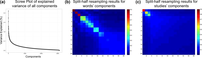
Variance explained and reproducibility (via split‐half resampling; SHR) of latent semantic components. (a) The Scree plot shows the explained variance per component for all 3,112 components. (b and c) Heatmaps of correlations between component scores after SHR, where (b) shows average (absolute) correlations after SHR for the words component scores and (c) shows the average (absolute) correlations after SHR for the studies component scores; only components 1 through 20 are shown. Both the Scree plot and the heatmap for the studies component scores suggest three high variance and highly reproducible components. The heatmap for the words component scores also show that the first three components are highly reproducible, but also that Components 4 and 5 are reproducible in the words component scores [Color figure can be viewed at http://wileyonlinelibrary.com]
To help interpret the components of our semantic space, we used the words and studies at the extremes (i.e., highest contributing variance) for each component (Figure 3 for extreme words; Supporting Information, Tables 1–5 for extreme studies). Table 1 shows the total and relative number of studies and words per cluster. As with the components, the most (and least) frequent words within each cluster help us interpret the cluster's meaning (Supporting Information, Table 6). Furthermore, we also identified the words closest to the barycenter of each cluster (across all five dimensions; Supporting Information, Table 7). We also provide the titles and PubMed IDs of the twenty studies closest to the barycenter of each cluster in Supporting Information, Tables 8–13 as well as the overall “most average” and “most unique” studies and terms in Supporting Information, Table 14. Component maps—which present two components at a time—are presented in Figure 2. We present component maps of the words and studies separately. In each map, we color each dot (i.e., a study or word) by its associated cluster. Components 1, 2, and 3 are visualized in Figure 2a–d. We show Components 4 and 5 separately from the other components (Figure 2e,f) because studies on Components 4 and 5 constitute a single cluster (see next section). Brain maps for the components are presented in Figure 3, and brain maps for clusters are presented in Figure 4. In Results, the components and clusters are first referred to by numbers: The component number reflects its rank order (by variance), but the cluster numbers are arbitrary. We provide interpretations of components and names for clusters after their descriptions.
Figure 3.
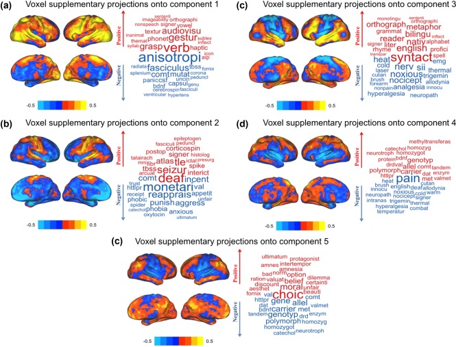
Visualization of brain maps, per component, as predicted (via supplementary projections) by the words × studies component scores (left) and a word cloud that shows some words that either loads on the positive or negative axis (right). (a) The projected map for Component 1 shows that the positive side (marked in red) is associated with the left temporal lobe, bilateral occipito‐temporal, and parietal regions, while the negative side (marked in blue) is associated with many subcortical structures. (b) The projected maps for Component 2 show that the positive side is associated with bilateral somatosensory areas and the right cerebellum (not rendered in surface plots), while the negative side is associated with subcortical structures as well as medial prefrontal cortex. (c) The projected brain maps for Component 3 show that the positive side is associated with the left lateralized language‐related areas while the negative side is associated with somatosensory cortex in addition to the brainstem (not rendered in surface plots). (d) The projected map for Component 4 shows that the positive side is associated with medial structures of parietal areas (precuneus) while the negative side is associated with bilateral somato‐sensory areas as well as the insular cortex and brainstem (not rendered in surface plots). (e) The projected brain maps for Component 5 show that the positive side is associated with the posterior cingulate and medial prefrontal cortices while the negative side is associated with bilateral somato‐sensory areas and the brainstem (not rendered in surface plots) [Color figure can be viewed at http://wileyonlinelibrary.com]
Table 1.
The total number of studies and terms per cluster
| Cluster | #Studies (%) | #Terms (%) | Brief description |
|---|---|---|---|
| 1 | 1,569 (14.4%) | 351 (11.3%) | Knowledge representation & language processing |
| 2 | 2,272 (20.8%) | 720 (23.1%) | Development, lifespan and disorders |
| 3 | 728 (6.7%) | 347 (11.1%) | Sensation, movement and action |
| 4 | 3,159 (28.9%) | 1019 (32.7%) | Cognition & psychology |
| 5 | 2,927 (26.9%) | 612 (19.7%) | Decision, emotion, & substance use |
| 6 | 243 (2.2%) | 65 (2.1%) | Imaging genetics |
| All | 10,898 | 3,114 |
Note. Our analyses revealed six clusters. The total number of studies and terms per cluster are provided. Furthermore, we provide a description that helps characterize the contents of each cluster.
Figure 2.
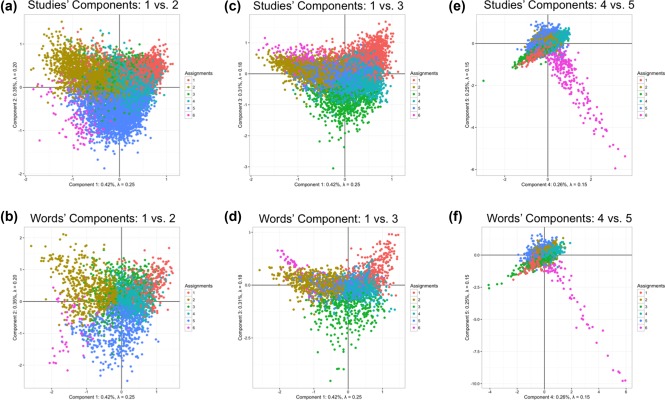
Visualization of the semantic space of functional neuroimaging literature. Component scores for both the words and the studies on Components 1–5 are visualized in a series of 2D figures. Axes are components and individual dots represent either a particular study or particular word. Words and studies are colored by which cluster they belong to and thus illustrate the large subdomains within fMRI. (a) and (b) show the words and studies (respectively) component scores for Components 1 (horizontal) and 2 (vertical). (c) and (d) show the words and studies (respectively) component scores for Components 1 (horizontal) and 3 (vertical). 2 (e) and (f) show the words and studies (respectively) component scores for Components 4 (horizontal) and 5 (vertical). While most words and studies form large groups within the axes, Components 4 and 5 show a highly specific subset of words and studies, of which nearly all are assigned to Cluster 6 (typically fMRI studies that include genetic and molecular terms) [Color figure can be viewed at http://wileyonlinelibrary.com]
Figure 4.
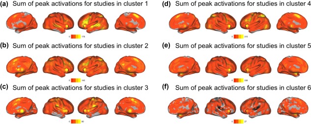
Visualization of brain maps, per cluster, computed as the sum of peak activations for all studies within a particular cluster. (a) Summed activations of individual studies in Cluster 1 (knowledge representation and language processing) showed in the bilateral peaks in the frontal and temporal lobes—which are often associated with language and knowledge representation—in addition to a peak area in the anterior cingulate cortex. (b) Summed peak activations of studies in Cluster 2 (development, lifespan and disorders) showed a diffuse pattern of reported activations in frontal and parietal areas, as well as subcortical regions. (c) Summed peak activations of studies in Cluster 3 (sensation, movement and action) showed in bilateral somatosensory areas and the thalamus. (d) Summed peak activations of studies in Cluster 4 (cognition and psychology) showed in the mid‐line and bilateral areas in frontal regions, in addition to bilateral occipito‐temporal regions. (e) Summed peak activations of Cluster 5 (decision, emotion, and substance use) appeared in subcortical areas and medial frontal regions. (f) Summed peak activations of Cluster 6 (imaging genetics) showed almost entirely subcortical areas [Color figure can be viewed at http://wileyonlinelibrary.com]
3.1. Components
Component 1's words and studies can be seen in Figure 2a,b. Words at extreme positive and negative sides of Component 1, as well as the projected brain maps for Component 1 are shown in Figure 3a. The projected brain map for Component 1 (Figure 3a) show that (a) The positive side of Component 1 is associated with the left temporal lobe, bilateral occipito‐temporal, and parietal regions, and (b) the negative side of Component 1 is associated with many subcortical structures. Component 1 generally reflects basic science research on the positive side to clinical/translational neuroimaging research on the negative side (Figure 2a,b). While the basic science research is more associated with cortical structures, the clinical/translational research is more linked with subcortical structures (Figure 3a).
Component 2's words and studies can be seen in Figure 2a,b. Words at the extreme positive and negative sides of Component 2, as well as the projected brain map for Component 2 are shown in Figure 3b. The projected brain maps for Component 2 show that (a) the positive side of Component 2 is associated with bilateral somatosensory areas and the right cerebellum and (b) the negative side of Component 2 is associated with subcortical structures as well as medial prefrontal cortex. Component 2 generally reflects a methodological spectrum that ranges from cognitive tasks on the negative side to multi‐modal imaging (e.g., structural–functional association) on the positive side. The negative—and more densely populated—side of Component 2 is more associated with studies on affect and emotion and similar study types (Figure 2a,b) with projections in subcortical and prefrontal cortex, whereas the positive side of Component 2 is linked to studies that rely on multi‐modal imaging and other related methodologies and somatosensory, temporal, and cerebellar projections (Figure 3b).
Component 3's words and studies can be seen in Figure 2c,d. Words at the extreme positive and negative sides of Component 3, as well as the projected brain maps for Component 3 are shown in Figure 3c. The projected brain maps for Component 3 show that (a) the positive side of Component 3 is associated with the left lateralized language‐related areas (e.g., temporal and frontal areas known as Broca's Area and Wernicke's Area) and (b) the negative side of Component 3 is associated with somatosensory cortex in addition to the brainstem. Component 3 generally reflects low‐to‐high level of cognition; studies about higher order cognitive processes (especially linguistics) are on the positive side of Component 3 (with cortical projections to the bilateral temporal and frontal regions; Figures 2c,d and 3c), whereas studies on lower order cognitive processes (such as sensation, perception, and direct sensory stimulation) are on the negative side of Component 3 (and also projects to the bilateral somatosensory areas and the brainstem in addition to the left cerebellum; Figures 2c,d and 3c).
Components 4's and 5's words and studies can be seen in Figure 2e,f and show a highly distinct pattern from the other components, mostly driven by words and studies related to molecular, genetic, and genomic neuroimaging studies. Words at the extreme positive and negative sides of Components 4 and 5, and the projected brain maps for Components 4 and 5 are shown in Figure 3d,e. The brain maps for Component 4 (Figure 3d) show that (a) the positive side of Component 4 is associated with medial structures of parietal areas (precuneus) and (b) the negative side of Component 4 is associated with bilateral somato‐sensory areas and the insular cortex and brainstem. The brain maps for Component 5 (in Figure 3e) show that (a) the positive side of Component 5 is associated with the posterior cingulate and medial prefrontal cortices and (b) the negative side of Component 5 is associated with bilateral somato‐sensory areas and the brainstem. Components 4 and 5 showed a distribution of words and studies that makes a near 45° angle between Components 4 and 5 that extended out from the origin. These words and studies were almost entirely molecular, genetic, and genomic neuroimaging (i.e., “imaging genetics”) studies. While studies on Component 4 are more associated with genetic contributions to cognition in healthy populations, by contrast, the projections to parietal and frontal regions studies on Component 5 were more associated with genetic contributions in disordered populations with projections to bilateral somatosensory regions.
3.2. Clusters
Cluster 1 contains studies/words primarily associated with language/speech production, comprehension, and disorders, as well as knowledge processing. Some examples include: decod, word, superior, auditori, languag, semant, percept, speech, recognit, complex (Supporting Information, Tables 6–8). Figure 2a,b shows that this cluster primarily lies on positive sides of Components 1 and 3. Summed peak activations of individual studies in this cluster are localized in the bilateral frontal and temporal regions—which are often associated with language and knowledge representation—in addition to the anterior cingulate cortex (Figure 4a). Cluster 1 represents the studies that mainly investigate knowledge representation and language processing and we henceforth refer to Cluster 1 as knowledge representation and language processing.
Cluster 2 contains studies/words associated with developmental, lifespan, and aging studies, and their respective disorders. Some examples include patient, differ, chang, healthi, age, structur, breakdown, degen, ecnp, epidemiolog (Supporting Information, Tables 6, 7, and 9). Figure 2a,b shows that this cluster primarily loads on the negative side of Component 1 and on the positive side of Component 2. Summed peak activations of studies in this cluster (Figure 4b) showed a diffuse pattern of activations in the frontal and parietal areas, and in the subcortical regions. Cluster 2 represents studies that mainly investigate developmental and adult lifespan research in addition to brain disorders and we henceforth refer to Cluster 2 as developmental, lifespan, and disorders.
Cluster 3 contains studies/words primarily associated with sensation (cutaneous and olfaction) and movement. Some examples include motor, pain, movement, hand, stimul, sensori, thalamus, somatosensori, reflex, anesthet (Supporting Information, Tables 6, 7, and 10). Figure 2c,d shows that this cluster loads primarily on the negative side of Component 3. Summed peak activations of studies in this cluster (Figure 4c) showed in the bilateral somato‐sensory areas and the thalamus. Cluster 3 represents studies that mainly investigate sensation, movement and action and we henceforth refer to Cluster 3 as sensation, movement, and action.
Cluster 4 contains studies/words associated with more “traditional” aspects of human cognitive neuroscience: those rooted in cognitive and experimental psychology (i.e., they rely primarily on behavioral tasks to examine neural correlates). Some examples include: activ, function, task, area, fmri, network, memori, effect, visual, decay (Supporting Information, Tables 6, 7, and 11). Figure 2a,c shows that Cluster 4 is closest to the origin point across all components with no apparent trend toward any axis. Summed peak activations of studies in this cluster (shown in Figure 4d) showed in the mid‐line and bilateral frontal regions, in addition to bilateral occipito‐temporal region. Cluster 4 represents the majority of cognition and psychological‐based functional neuroimaging research and we henceforth refer to Cluster 4 as cognition and psychology.
Cluster 5 contains studies/words that describe affective processes, such as emotional responses and decision‐making, but also includes a number of studies and words related to substance use disorders and mood disorders. Cluster 5 includes the words: emot, prefront, reson, cingul, examin, medial, amygdala, negat, social, diminish, take (Supporting Information, Tables 6, 7, and 12). Figure 2a,b shows that this cluster lies mostly on the negative side of Component 2. Summed peak activations of Cluster 5 (Figure 4e) appeared in subcortical areas and medial frontal regions. Cluster 5 represents studies that mainly investigate decision‐making, emotions and substance use (or abuse) and we henceforth refer to Cluster 5 as decision, emotion, and substance use.
Cluster 6 loads almost entirely and exclusively on both Components 4 and 5 (Figure 2e,f). Cluster 6 contains words such as: variat, genet, dopamin, gene, carrier, allel, genotyp, receptor, polymorph, dopaminerg, comt, serotonin, apo, norepinephrine (Supporting Information, Tables 6, 7, and 13). Summed peak activations of Cluster 6 (Figure 4f) showed almost entirely in the subcortical areas. Cluster 6 represents a unique dimension (i.e., Components 4 and 5) of molecular, genetic, and genomic neuroimaging (“imaging genetics”) studies and we henceforth refer to Cluster 6 as “imaging genetics.”
3.3. Temporal effects of clusters
Upon completion of the analyses, there were two clusters that stood out: (a) Cluster 4 (cognition and psychology)—which is essentially the “average” neuroimaging study because it is centered roughly on the origin of the components—and (b) Cluster 6 (imaging genetics)—which is comprised of the studies that define Components 4 and 5). Notably, Cluster 4 (cognition and psychology) reflects the origins of neuroimaging use (i.e., cognitive psychology), whereas Cluster 6 (imaging genetics) reflects the current state‐of‐the‐art (i.e., translational and interdisciplinary work).
Figure 5 shows the relative frequency of the number of studies in each cluster sorted by year. Cluster 4 (cognition and psychology) accounts for a substantial amount of studies in the earlier years. For example, in the year 2000, approximately 50% of all neuroimaging studies (in Neurosynth) were in Cluster 4 (cognition and psychology). On the other hand, Cluster 5 (decision, emotion, & substance use) started as a small proportion of all neuroimaging studies in the earlier years, but now accounts for nearly 33% of all studies. We discuss the temporal properties of these clusters further in Section 4.
Figure 5.
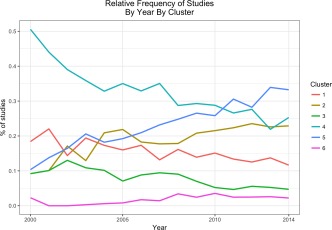
The proportion of studies within each cluster over time. Cluster 4 (cognition and psychology) was, and still generally is the core of fMRI research and as such comprises a substantial proportion of the literature. Though Cluster 4 (cognition and psychology) remains very large, it has decreased over time. Both Cluster 5 (decision, emotion, substance use) and Cluster 2 (developmental, lifespan, disorders) have shown a considerable increase over time and now comprise, respectively, comparable proportions of the literature as Cluster 4 (cognition and psychology) [Color figure can be viewed at http://wileyonlinelibrary.com]
3.4. Correlations with maps in Yeo et al. (2015)
In Yeo et al. (2015), a hierarchal Bayesian model was applied to 10,449 experimental contrasts in the BrainMap database to estimate the probability that each pre‐defined task category would engage a specific cognitive component, and the probability that each cognitive component would engage brain regions (represented by voxels). Correlations between our component and cluster maps and Yeo et al. (2015)'s 12‐component cognitive maps were computed using a custom script. We first downloaded the maps from Neurovault (http://neurovault.org/collections/866/, last accessed June 7, 2017). We only included the nonzero voxels from the component maps to exclude all non‐valid voxels (i.e., outside the brain).
Figure 6 shows the correlations between our maps and the maps from Yeo et al (2015). We refer to Yeo et al.'s (2015) components as, for example, Yeo Component 1 (YC1) or Yeo Component 6 (YC6) while we refer to our own components as “Component 1” or “Component 5.” There were several correlations of note for both the components (Figure 6a) and the clusters (Figure 6b). To note, although the magnitudes of those correlations are interpretable, the sign (or direction) of the correlation are not easily interpretable.
Figure 6.
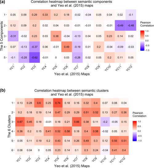
Correlations between the maps generated by Yeo et al., (2015) and (a) our components or (b) our clusters. There are some notably high similarities between our brain maps (which were generated conditional to the latent semantic space) and the Yeo et al., (2015) maps, such as the Yeo components 11 and 12 with our Component 2 (see a), and the Yeo components 1 and 7 with our Cluster 3 (see b) [Color figure can be viewed at http://wileyonlinelibrary.com]
Figure 6a shows the strong correlations between our Component 2 and YC11 and YC12. Both maps show strong association with bilateral subcortical structures (e.g., amygdala and striatum) in addition to their relationship with subcortical‐related functions such as emotions and affect. Also, there is a strong correlation between our Component 3 and YC5 because both maps show strong association with temporal and frontal activations in addition to their relationships with semantic knowledge and language processing. Furthermore, there is a strong correlation between our Component 4 and YC6 because both maps show strong associations with medial parietal and frontal areas (commonly known as the frontal‐parietal network; Smith et al., 2009).
Similar to the components, correlations between our clusters and the Yeo components are illustrated in Figure 6b. Our Cluster 1 is most correlated with YC 5 followed by YC3, all of which have activations in the temporal and frontal regions and are generally involved with knowledge representation and higher order semantic processing. Our Cluster 3 is correlated with YC1 followed by YC7, both of which have activations in somatosensory areas and are involved in sensation and movement processing. Our Clusters 5 are both correlated with YC11 and YC12, all of which are associated with activations in subcortical structures and are associated with tasks that involve some aspect of affective or emotional processing. Although our Cluster 6 also share the same regions (and is most similar to YC11 and YC12), it comes mostly from molecular and genetic studies.
3.5. Recommendation engine
Finally, we provide a simple tool in R as a Shinyapp that works as a “recommendation engine” akin to preference and ratings systems (e.g., for movie preferences, shopping, or internet searches). While the app has many current and planned features, we only discuss the recommendation portion here. Our recommendation tool uses a distance‐based search to retrieve papers (PMIDs) that are the most semantically similar to a given paper (PMID). Specifically, users only need to provide (a) a PMID of a paper of interest and (b) how many N similar papers to select. Our recommendation tool then provides the N papers closest to the target paper. Additionally, in the same way as for the papers, users can input a term of interest and retrieve the N closest terms. In both cases, we also provide additional information such as to which primary domain (cluster) a study or term belongs. The recommendation is based on the component scores of the first five components (see Results). This recommendation engine, however, works based on the results in this paper and not the most recent version of Neurosynth. However, we provide code for all of our work including the recommendation tool and thus all results and recommendations can be updated as Neurosynth is updated. The recommendation engine with a brief description and how‐to are available at the following address: http://bit.ly/neurosanity.
4. DISCUSSION
In recent years, there have been many meta‐analyses, mega‐analyses (analyses of pooled data across many studies), and other large‐scale analyses of data within neuroimaging. In general, the aims of such analyses are to (a) test or refute findings and hypotheses (Wager, Lindquist, & Kaplan, 2007), (b) build a consensus around particular models, hypotheses, or theories (Salimi‐Khorshidi et al., 2009), (c) estimate consistency of findings (Wager, Lindquist, Nichols, Kober, & Van Snellenberg, 2009), (d) help define related brain regions and networks (Toro, Fox, & Paus, 2008; Mesmoudi et al., 2013), (e) interpret functional maps (Laird et al., 2011), or (f) segment the brain in new ways with resting‐state fMRI measurements (Yeo et al., 2011; Power et al., 2011) or using massive multimodal data (Glasser et al., 2016).
Using the meta‐analytic cognitive component maps from Yeo et al. (2015) as a reference point to compare with our maps, we showed a substantial overlap between many of our maps and maps from Yeo et al. (2015). However, our meta‐analytic maps were predicted from the semantic space (i.e., abstracts) of the functional neuroimaging literature, whereas other authors took a more brain‐centric approach, for examples: network‐ and meta‐maps generated by with resting state fMRI (Yeo et al., 2011; Power et al., 2011) or via meta‐analysis of data from hundreds or even thousands of studies (Poldrack et al., 2012; de la Vega et al., 2016; Yang et al., 2015, 2016).
Our components explain the primary sources of variance of language used: in the field at large (i.e., Component 1), for methodological tools (i.e., Component 2), in various aspects of cognition (i.e., Component 3), and in relatively new studies with highly‐specific terminology (i.e., Components 4 and 5). With supplementary projections we also showed that these language‐based components are frequently associated with particular reported brain regions. While the components indicate language variation and gradients, our clusters define the boundaries of functional neuroimaging into specific—albeit large—subdomains. Furthermore, our analyses revealed that there are, perhaps, biases or preferentially studied brain areas per domain (i.e., clusters).
Parts of our semantic space also reflect, to a degree, current debates such as the distinctions between “neurological versus psychiatric brain disorders” (White, Rickards, & Zeman, 2012). For example, Crossley, Scott, Ellison‐Wright, and Mechelli (2015) recently used CBMA of voxel‐based morphometric (VBM) studies to show a “neuroimaging‐based” evidence for the biological distinctions between neurological versus psychiatric disorders (Crossley et al., 2015). Our components show that neuroimaging studies in neurology and psychiatry do not use the same terminology and thus could be a source of the “versus” argument between neurological and psychiatric studies with respect to reported brain regions. As an illustration of this contention, we have selected some of the same neurology and psychiatry related terms used by Crossley et al., (2015) to highlight particular features of our components. First, all the words related to psychiatric or neurological disorders (Supporting Information, Table 15) appear on the negative side of Component 1—a configuration that supports our interpretation of a spectrum from basic science to applied and clinical neuroimaging. Furthermore, the neurological and psychiatric terms from Crossley et al., (2015) oppositely load on both Components 2 and 4 (Supporting Information, Table 15): a configuration that reflects overall differences in patterns of terminology between neurological and psychiatric studies and thus expresses a dissociation of neurological studies and their regions (such as sensorimotor cortices and insula; in red) from psychiatric studies and their regions (such as limbic and prefrontal areas; in blue) as seen in Figure 3b. Further discrepant terminology can be seen in Supporting Information, Table 16.
Furthermore, the positions—and contents—of our clusters reveal a broad configuration of the neuroimaging literature. Cluster 4 (cognition and psychology) is the closest to the barycenter (origin of the axes across all components) and thus represents the average or most common neuroimaging study. This interpretation is supported by Cluster 4 (cognition and psychology) because it contains a substantial proportion of words and studies (∼33% of words and ∼29% of studies, see Table 1). Thus, much of the neuroimaging literature has been—and appears to still be—rooted in the approaches from cognitive and psychological domains. Summed peak activations of studies in this cluster (shown in Figure 4d) show a high association with a wide set of cortical areas in the medial and bilateral frontal, occipital and subcortical regions that are associated with task performance. We also see opposition of clusters and this suggests that these are the sources of variance for our components. For example, Cluster 5 (decision, emotion, and substance use) is opposed to all other clusters on Component 2 (Figure 2a,b)—a pattern that further supports the neurological vs. psychiatric dissociation of Component 2. Summed peak activations of studies in this cluster (shown in Figure 4e) show high association with the subcortical areas and medial frontal regions that are generally associated with emotional processing and decision‐making process. Similarly, Cluster 3 (sensation, movement, and action) is opposed to all other clusters on Component 3 (Figure 2c,d)—a component that, as we previously noted, expresses a spectrum from low‐to‐high level processing. Summed peak activations of studies in this cluster (shown in Figure 4c) show high association with the bilateral somatosensory areas and the thalamus. Furthermore, Cluster 6 (imaging genetics) is almost entirely defined by the unique configuration of both Components 4 and 5 (Figure 2e,f). Not only does Cluster 6 reflects a unique subfield of neuroimaging, but it also indicates that “imaging genetics” uses an almost exclusive set of words, different from the vocabulary of the rest of neuroimaging (cf., the 45° angle from Components 4 and 5). Summed peak activations of Cluster 6 (Figure 4f) are almost entirely associated with subcortical areas. Finally, both Clusters 4 (cognition and psychology) and 5 (decision, emotion, and substance use) proportionally explain over half of the literature at any given time (Figure 5).
Our clusters and their respective brain maps are consistent with results of other meta‐analysis. The activation map of Cluster 1 (knowledge representation and language processing; Figure 4a) is similar to other published meta‐analytic maps and reviews of language processing and semantic representation (Binder, Desai, Graves, & Conant, 2009; Bookheimer, 2002; Fedorenko & Thompson‐Schill, 2014; Price, 2010, 2012). The activation map of Cluster 3 (Sensation, Movement and Action; Figure 4c) is similar to other maps from studies investigating pain localization (Amanzio, Benedetti, Porro, Palermo, & Cauda, 2013; Friebel, Eickhoff, & Lotze, 2011; Perini, Bergstrand, & Morrison, 2013; Schomers & Pulvermüller, 2016; Vierck, Whitsel, Favorov, Brown, & Tommerdahl, 2013) in addition to the somatosensory co‐activation network (Smith et al., 2009). Finally, the activation map of Cluster 5 (decision, emotion, and substance use; Figure 4e) is also highly similar to the map of the structures involved in different aspects of emotional processing and decision‐making (Bartra, McGuire, & Kable, 2013; Buhle et al., 2014; Etkin & Wager, 2007; Lindquist, 2010; Phan, Wager, Taylor, & Liberzon, 2002).
Many meta‐analyses and meta‐analytic tools for neuroimaging have a common (even if unstated) goal: to help homogenize our understanding of the literature and through this homogenization help define ontologies (Poldrack & Yarkoni, 2016; Poldrack et al., 2011) so that we can relate brain function to cognition. However, with many tools at our disposal, there are known biases in neuroimaging (Jennings & Van Horn, 2012) and the language we use can make building such ontologies difficult. With a well‐defined common language and homogenization of reporting results, fields such as genomics can provide a more robust assessment of the relationship between studies and the roles of particular genetic effects (Ailem et al., 2016).
Based on the analysis of term co‐occurrences in the abstracts of 10,898 neuroimaging articles, we have identified a highly reliable set of dimensions and subfields that define the underlying semantic space of the neuroimaging field. Most researchers tend to stay within their specialized domain (by using specific key terms common to their field) and this behavior may restrict what they can conclude and how they report their findings, because they use a preferred or required terminology. In fact, Clusters 2 (development, lifespan, and disorders) and 5 (decision, emotion, and substance use), and Components 1 and 2 show that there are language barriers between different types of clinical and experimental studies that could preclude thorough reviews of relevant literature (see examples in Supporting Information, Table 16).
Because such diverse terminologies and highly specialized fields could cause researchers to overlook relevant work in domains related and unrelated to their own, two recent approaches—in addition to our own—have been proposed: Papr (McGowan et al., 2017) and MAPBOT (Yuan, Taylor, Alvarez, Mishra, & Biswal, 2017). In general, our approach, Papr, and MAPBOT all aim to help users navigate literature in an easier way and to better understand the relationships between studies. Furthermore, all these techniques use multivariate tools based on the singular value decomposition. We describe and then compare each to our approach below.
Papr was recently released to help researchers find preprints on bioRxiv that may be of interest to them. With Papr, users can move through a semantic subspace to find articles whose abstract is similar to a target abstract, as well as locate other users with similar interest.2 Papr provides for bioRxiv some of the mechanisms (e.g., similarity and recommendation of studies) that our approach does for Neurosynth. There are, however, several major differences between our approach and Papr. First, Papr is a tool for bioRxiv while our study and many of our analyses are specifically tailored to the functional neuroimaging literature (covered by Neurosynth). Second, Papr emphasizes only study similarity. While our approach emphasizes study similarity and high‐level organization of the functional neuroimaging literature, we also use the terms. The difference between Papr and our approach stems from the choice of multivariate method used: Papr uses PCA, whereas we use CA. CA is a bifactor technique suited to jointly accommodate the rows (studies) and columns (terms) of a matrix comprising positive values. Also we took the analysis of the semantic subspace further than Papr by clustering the literature into high‐level domains in order to illustrate the broad configuration of the functional neuroimaging literature.
Similar to our study, MAPBOT utilized the Neurosynth database. MAPBOT helps researchers navigate relevant studies in Neurosynth, but conditional to a region of interest. For example, in their paper, Yuan et al., (2017) use a thalamic mask to generate a voxel × term matrix. MAPBOT extracts only the studies in Neurosynth that report voxels within an a priori mask to create a voxel × term matrix. MAPBOT then decomposes that voxel × term matrix with non‐negative matrix factorization (a technique, like CA, that was designed for use with strictly positive values). MAPBOT's goal is to provide better parcellation of regions, with richer content (i.e., terms) to help researchers understand, for examples, the functional or behavioral associations of parcellations within a mask. There are several major differences between our approach and MAPBOT. First is that MAPBOT analyzes voxel × term content. However, MAPBOT is restricted to a priori masks; that is, users must select a specific partition of voxel space. By doing so, MAPBOT cannot detect similar semantic content across voxel content. Our approach first analyzes studies × term content, and then projects (predicts) voxel content. Our approach incorporates studies, terms, and voxels for all available studies as opposed to a specific subset.
In summary, Papr is a tool to assess semantic similarity between abstracts in bioRxiv, MAPBOT parcellates a priori defined brain regions by using semantic content, whereas our approach first assesses semantic similarity, then partitions (clusters) the semantic subspace, next it predicts voxel data from the semantic subspace, and finally assigns voxels to particular clusters. While both Papr and MAPBOT provide some tools to better navigate and search the literature, both are lacking the key features and information we provide here. We believe that our approach to structuring the functional neuroimaging literature, and our current version of a recommendation engine, is critical to both help organize the field and to help researchers navigate the literature.
5. CONCLUSIONS
To conclude, our work shows that different domains use different patterns of words, and that studies within these domains also report (or perhaps only study specific but) common brain areas. We believe that neuroimaging—and all of the domains that use and contribute to neuroimaging—would benefit from a broader harmonization of their terminology (à la the COBIDAS appendix on how to report routine fMRI analyses; Nichols et al., 2016) to put the field on the path toward formal ontologies (Poldrack & Yarkoni, 2016). However, there are barriers to achieve such ontologies (see examples in Supporting Information, Table 16). One such barrier is time and it poses difficult questions, such as should we go back to older papers and “correct” terminology (e.g., addiction vs. substance use disorder). Another barrier is language itself because many terms have a variety of uses across disciplines (e.g., to recollect) and the same concepts could have multiple terms and used in different ways depending on factors such as stylistic choices by the authors (e.g., marijuana vs. cannabis). Another limitation is that some of the automated language tools commonly used (including by us) cannot always detect that certain stems have the same meaning (hippocampi vs. hippocampus). Formal and more rigorous ontologies—such as those in genomics—and tools more sensitive to the peculiarities of language will be required as our field moves forward and connects brain imaging to a variety of other modalities (e.g., genetics; Cioli, Abdi, Beaton, Burnod, & Mesmoudi, 2014; Rizzo et al., 2016), but will require effort from a variety of disciplines to harmonize and standardize terminology.
Supporting information
Additional Supporting Information may be found online in the supporting information tab for this article.
Supporting Information
ACKNOWLEDGMENTS
The authors would like to thank Micaela Chan and Jenny Rieck for their feedback on previous versions of this manuscript. They also greatly appreciate all the public commentary that they received provided by many individuals in various formats (e.g., Twitter, brainhack Slack channels).
Alhazmi FH, Beaton D, Abdi H. Semantically defined subdomains of functional neuroimaging literature and their corresponding brain regions. Hum Brain Mapp. 2018;39:2764–2776. 10.1002/hbm.24038
Authors note: The majority of the work was done while FA and DB were at The University of Texas at Dallas, and completed while DB was at the Rotman Research Institute. FA is now at The Graduate Center, CUNY.
Footnotes
We used absolute correlation because there can be trivial sign flips between subsamples of data, so the sign is irrelevant but the magnitude of the correlation is relevant.
Currently there is an offline version of Papr here: https://github.com/jtleek/papr. During the writing of our manuscript, a “live” version of Papr was available but may no longer be “live”: https://jhubiostatistics.shinyapps.io/papr/
Contributor Information
Fahd H. Alhazmi, Email: falhazmi@gradcenter.cuny.edu.
Derek Beaton, Email: dbeaton@research.baycrest.org.
Hervé Abdi, Email: herve@utdallas.edu.
REFERENCES
- Abdi, H. , & Béra, M. (2014). Correspondence analysis In Encyclopedia of Social Network Analysis and Mining (pp. 275–284). New York, NY: Springer. [Google Scholar]
- Ailem, M. , Role, F. , Nadif, M. , & Demenais, F. (2016). Unsupervised text mining for assessing and augmenting GWAS results. Journal of Biomedical informatics, 60(February), 252–259. [DOI] [PubMed] [Google Scholar]
- Amanzio, M. , Benedetti, F. , Porro, C. A. , Palermo, S. , & Cauda, F. (2013). Activation likelihood estimation meta‐analysis of brain correlates of placebo analgesia in human experimental pain. Human Brain Mapping, 34(3), 738–752. [DOI] [PMC free article] [PubMed] [Google Scholar]
- Bartra, O. , McGuire, J. T. , & Kable, J. W. (2013). The valuation system: A coordinate‐based meta‐analysis of BOLD fMRI experiments examining neural correlates of subjective value. NeuroImage, 76, 412–427. [DOI] [PMC free article] [PubMed] [Google Scholar]
- Beaton, D. , Fatt, C. R. C. , & Abdi, H. (2014). An ExPosition of multivariate analysis with the singular value decomposition in R. Computational Statistics & Data Analysis, 72, 176–189. [Google Scholar]
- Benzécri, J. P. (1976). History and prehistory of data analysis. III: Era piscatoria (French). Les Cahiers de l'Analyse Des Données, 1, 221–241. [Google Scholar]
- Binder, J. R. , Desai, R. H. , Graves, W. W. , & Conant, L. L. (2009). Where is the semantic system? A critical review and meta‐analysis of 120 functional neuroimaging studies. Cerebral Cortex (New York, N.Y. : 1991), 19(12), 2767–2796. [DOI] [PMC free article] [PubMed] [Google Scholar]
- Bookheimer, S. (2002). Functional MRT of language: New approaches to understanding the cortical organization of semantic processing. Annual Review of Neuroscience, 25(1), 151–188. [DOI] [PubMed] [Google Scholar]
- Buhle, J. T. , Silvers, J. A. , Wager, T. D. , Lopez, R. , Onyemekwu, C. , Kober, H. , … Ochsner, K. N. (2014). Cognitive reappraisal of emotion: A meta‐analysis of human neuroimaging studies. Cerebral Cortex (New York, N.Y. : 1991), 24(11), 2981–2990. [DOI] [PMC free article] [PubMed] [Google Scholar]
- Calinski, T. , & Harabasz, J. (1974). A dendrite method for cluster analysis. Communications in Statistics ‐ Theory and Methods, 3(1), 1–27. [Google Scholar]
- Churchill, N. W. , Oder, A. , Abdi, H. , Tam, F. , Lee, W. , Thomas, C. , … Strother, S. C. (2012). Optimizing preprocessing and analysis pipelines for single‐subject fMRI. I. Standard temporal motion and physiological noise correction methods. Human Brain Mapping, 33(3), 609–627. [DOI] [PMC free article] [PubMed] [Google Scholar]
- Cioli, C. , Abdi, H. , Beaton, D. , Burnod, Y. , & Mesmoudi, S. (2014). Differences in human cortical gene expression match the temporal properties of large‐scale functional networks. PLoS ONE, 9(12), e115913–e115928. [DOI] [PMC free article] [PubMed] [Google Scholar]
- Crossley, N. A. , Scott, J. , Ellison‐Wright, I. , & Mechelli, A. (2015). Neuroimaging distinction between neurological and psychiatric disorders. British Journal of Psychiatry, 207(05), 429–434. [DOI] [PMC free article] [PubMed] [Google Scholar]
- de la Vega, A. , Chang, L. J. , Banich, M. T. , Wager, T. D. , & Yarkoni, T. (2016). Large‐scale meta‐analysis of human medial frontal cortex reveals tripartite functional organization. Journal of Neuroscience, 36(24), 6553–6562. [DOI] [PMC free article] [PubMed] [Google Scholar]
- Desgraupes, B. (2015). clusterCrit: clustering indices. Retrieved from http://cran.r-project.org/package=clusterCrit
- Escofier‐Cordier, B. (1965). L'Analyse des Correspondences. Doctoral Dissertation: Université de Rennes.
- Etkin, A. , & Wager, T. D. (2007). Functional neuroimaging of anxiety: A meta‐analysis of emotional processing in PTSD, social anxiety disorder, and specific phobia. American Journal of Psychiatry, 164(10), 1476–1488. [DOI] [PMC free article] [PubMed] [Google Scholar]
- Fedorenko, E. , & Thompson‐Schill, S. L. (2014). Reworking the language network. Trends in Cognitive sciences, 18(3), 120–127. [DOI] [PMC free article] [PubMed] [Google Scholar]
- Feinerer, I. (2011). Introduction to the tm Package Text Mining in R. R Vignette, 1–8. [Google Scholar]
- Fox, A. , Chang, L. , Gorgolewski, K. , & Yarkoni, T. (2014a). Bridging psychology and genetics using large‐scale spatial analysis of neuroimaging and neurogenetic data. bioRxiv. [Google Scholar]
- Fox, P. T. , Lancaster, J. L. , Laird, A. R. , & Eickhoff, S. B. (2014b). Meta‐analysis in human neuroimaging: Computational modeling of large‐scale databases. Annual Review of Neuroscience, 37(1), 409–434. [DOI] [PMC free article] [PubMed] [Google Scholar]
- Friebel, U. , Eickhoff, S. B. , & Lotze, M. (2011). Coordinate‐based meta‐analysis of experimentally induced and chronic persistent neuropathic pain. NeuroImage, 58(4), 1070–1080. [DOI] [PMC free article] [PubMed] [Google Scholar]
- Glasser, M. F. , Coalson, T. S. , Robinson, E. C. , Hacker, C. D. , Harwell, J. , Yacoub, E. , … Van Essen, D. C. (2016). A multi‐modal parcellation of human cerebral cortex. Nature, 536(7615), 171–178. [DOI] [PMC free article] [PubMed] [Google Scholar]
- Gorgolewski, K. J. , Varoquaux, G. , Rivera, G. , Schwarz, Y. , Ghosh, S. S. , Maumet, C. , … Margulies, D. S. (2015). NeuroVault.org: a web-based repository for collecting and sharing unthresholded statistical maps of the human brain. Frontiers in Neuroinformatics, 9. 10.3389/fninf.2015.00008 [DOI] [PMC free article] [PubMed] [Google Scholar]
- Greenacre, M. (2017). Correspondence analysis in practice (3rd ed.). CRC Press. [Google Scholar]
- Greenacre, M. J. (1984). Theory and applications of correspondence analysis. Academic Press. [Google Scholar]
- Jennings, R. G. , & Van Horn, J. D. (2012). Publication bias in neuroimaging research: Implications for meta‐analyses. Neuroinformatics, 10(1), 67–80. [DOI] [PMC free article] [PubMed] [Google Scholar]
- Laird, A. R. , Fox, P. M. , Eickhoff, S. B. , Turner, J. A. , Ray, K. L. , McKay, D. R. , … Fox, P. T. (2011). Behavioral interpretations of intrinsic connectivity networks. Journal of Cognitive Neuroscience, 23(12), 4022–4037. [DOI] [PMC free article] [PubMed] [Google Scholar]
- Laird, A. R. , Lancaster, J. L. , & Fox, P. T. (2005). BrainMap: The social evolution of a human brain mapping database. Neuroinformatics, 3(1), 065. [DOI] [PubMed] [Google Scholar]
- Lebart, L. L. , Salem, A. , & Berry, L. (1998). Exploring textual data. Springer; 10.1007/978-94-017-1525-6. [DOI] [Google Scholar]
- Lebart, L. , Morineau, A. , & Warwick, K. M. (1984). Multivariate descriptive statistical analysis; correspondence analysis and related techniques for large matrices. John Wiley. [Google Scholar]
- Lindquist, K. A. (2010). The brain basis of emotion: A meta‐analytic review. Dissertation Abstracts International, B: Sciences and Engineering, 71(4), 2744. [Google Scholar]
- McGowan, L. D. , Strayer, N. , & Leek, J. T. (2017). papr: Tinder for pre‐prints, a Shiny Application for collecting gut‐reactions to pre‐prints from the scientific community. Presented at useR!2017, Brussels, BE. Retrieved from https://channel9.msdn.com/Events/useR-international-R-User-conferences/useR-International-R-User-2017-Conference/papr-Tinder-for-pre-prints-a-Shiny-Application-for-collecting-gut-reactions-to-pre-prints-from-the-s
- Mesmoudi, S. , Perlbarg, V. , Rudrauf, D. , Messe, A. , Pinsard, B. , Hasboun, D. , … Burnod, Y. (2013). Resting state networks’ corticotopy: The dual intertwined rings architecture. PLoS ONE, 8(7), e67444. [DOI] [PMC free article] [PubMed] [Google Scholar]
- Mesmoudi, S. , Rodic, M. , Cioli, C. , Cointet, J. P. , Yarkoni, T. , & Burnod, Y. (2015). LinkRbrain: Multi‐scale data integrator of the brain. Journal of Neuroscience Methods, 241, 44–52. [DOI] [PMC free article] [PubMed] [Google Scholar]
- Murtagh, F. , & Legendre, P. (2014). Ward's hierarchical clustering method: Clustering criterion and agglomerative algorithm. Journal of Classification, 31(3), 274–295. [Google Scholar]
- Nichols, T. E. , Das, S. , Eickhoff, S. B. , Evans, A. C. , Glatard, T. , Hanke, M. , … Yeo, B. T. T. (2016). Best practices in data analysis and sharing in neuroimaging using MRI. bioRxiv, 54262. [DOI] [PMC free article] [PubMed] [Google Scholar]
- Nielsen, F. Å. A. (2003). The Brede database: A small database for functional neuroimaging. NeuroImage, 19, 2000–2001. [Google Scholar]
- Nielsen, F. A. , Hansen, L. K. , & Balslev, D. (2004). Mining for associations between text and brain activation in a functional neuroimaging database. Neuroinformatics, 2(4), 369–380. [DOI] [PubMed] [Google Scholar]
- Perini, I. , Bergstrand, S. , & Morrison, I. (2013). Where pain meets action in the human brain. Journal of Neuroscience, 33(40), 15930–15939. [DOI] [PMC free article] [PubMed] [Google Scholar]
- Phan, K. L. , Wager, T. , Taylor, S. F. , & Liberzon, I. (2002). Functional neuroanatomy of emotion: A meta‐analysis of emotion activation studies in PET and fMRI. NeuroImage, 16(2), 331–348. [DOI] [PubMed] [Google Scholar]
- Poldrack, R. A. , Kittur, A. , Kalar, D. , Miller, E. , Seppa, C. , Gil, Y. , … Bilder, R. M. (2011). The cognitive atlas: Toward a knowledge foundation for cognitive neuroscience. Frontiers in Neuroinformatics, 5(September), 1–11. [DOI] [PMC free article] [PubMed] [Google Scholar]
- Poldrack, R. A. , Mumford, J. A. , Schonberg, T. , Kalar, D. , Barman, B. , & Yarkoni, T. (2012). Discovering relations between mind, brain, and mental disorders using topic mapping. PLoS Computational Biology, 8(10), e1002707. [DOI] [PMC free article] [PubMed] [Google Scholar]
- Poldrack, R. A. , & Yarkoni, T. (2016). From brain maps to cognitive ontologies : Informatics and the search for mental structure. Annual Review of Psychology, 67(1), 587. [DOI] [PMC free article] [PubMed] [Google Scholar]
- Power, J. D. , Cohen, A. L. , Nelson, S. M. , Wig, G. S. , Barnes, K. A. , Church, J. A. , … Petersen, S. E. (2011). Functional network organization of the human brain. Neuron, 72(4), 665–678. [DOI] [PMC free article] [PubMed] [Google Scholar]
- Price, C. J. (2010). The anatomy of language: A review of 100 fMRI studies published in 2009. Annals of the New York Academy of Sciences, 1191(1), 62–88. [DOI] [PubMed] [Google Scholar]
- Price, C. J. (2012). A review and synthesis of the first 20years of PET and fMRI studies of heard speech, spoken language and reading. NeuroImage, 62(2), 816–847. [DOI] [PMC free article] [PubMed] [Google Scholar]
- R Core Team . (2017). R: A language and environment for statistical computing. R Foundation for Statistical Computing, Vienna, Austria. Retrieved from https://www.R-project.org/.
- Rizzo, G. , Veronese, M. , Expert, P. , Turkheimer, F. E. , & Bertoldo, A. (2016). Menga: A new comprehensive tool for the integration of neuroimaging data and the allen human brain transcriptome atlas. PLoS ONE, 11(2), e0148744–e0148720. [DOI] [PMC free article] [PubMed] [Google Scholar]
- Rubin, T. N. , Koyejo, O. , Gorgolewski, K. J. , Jones, M. N. , Poldrack, R. A. , & Yarkoni, T. (2016). Decoding brain activity using a large‐scale probabilistic functional‐anatomical atlas of human cognition. bioRxiv. [DOI] [PMC free article] [PubMed] [Google Scholar]
- Salimi‐Khorshidi, G. , Smith, S. M. , Keltner, J. R. , Wager, T. D. , & Nichols, T. E. (2009). Meta‐analysis of neuroimaging data: A comparison of image‐based and coordinate‐based pooling of studies. NeuroImage, 45(3), 810–823. [DOI] [PubMed] [Google Scholar]
- Schomers, M. R. , & Pulvermüller, F. (2016). Is the sensorimotor cortex relevant for speech perception and understanding? An integrative review. Frontiers in Human Neuroscience, 10(September). [DOI] [PMC free article] [PubMed] [Google Scholar]
- Smith, S. M. , Fox, P. T. , Miller, K. L. , Glahn, D. C. , Fox, P. M. , Mackay, C. E. , … Beckmann, C. F. (2009). Correspondence of the brain’ s functional architecture during activation and rest. Proceedings of the National Academy of Sciences of the United States of America, 106(31), 13040–13045. [DOI] [PMC free article] [PubMed] [Google Scholar]
- Strother, S. C. , Anderson, J. O. N. , Hansen, L. K. , Kjems, U. , Kustra, R. , Sidtis, J. , … Rottenberg, D. (2002). The quantitative evaluation of functional neuroimaging experiments: The NPAIRS data analysis framework. NeuroImage, 15(4), 747–771. [DOI] [PubMed] [Google Scholar]
- Toro, R. , Fox, P. T. , & Paus, T. (2008). Functional coactivation map of the human brain. Cerebral Cortex (New York, N.Y. : 1991), 18(11), 2553–2559. [DOI] [PMC free article] [PubMed] [Google Scholar]
- Van Essen, D. C. , Drury, H. A. , Dickson, J. , Harwell, J. , Hanlon, D. , & Anderson, C. H. (2001). An integrated software suite for surface‐based analyses of cerebral cortex. Journal of the American Medical Informatics Association, 8(5), 443–459. [DOI] [PMC free article] [PubMed] [Google Scholar]
- Van Essen, D. , Reid, E. , Gu, P. , & Harwell, J. (2009). Mining the neuroimaging literature using the SumsDB database: Stereotaxic coordinates and more! Frontiers in Neuroinformatics. [Google Scholar]
- Vierck, C. J. , Whitsel, B. L. , Favorov, O. V. , Brown, A. W. , & Tommerdahl, M. (2013). Role of primary somatosensory cortex in the coding of pain. Pain, 154(3), 334–344. [DOI] [PMC free article] [PubMed] [Google Scholar]
- Wager, T. D. , Lindquist, M. A. , Nichols, T. E. , Kober, H. , & Van Snellenberg, J. X. (2009). Evaluating the consistency and specificity of neuroimaging data using meta‐analysis. NeuroImage, 45(1), S210–S221. [DOI] [PMC free article] [PubMed] [Google Scholar]
- Wager, T. D. , Lindquist, M. , & Kaplan, L. (2007). Meta‐analysis of functional neuroimaging data: Current and future directions. Social Cognitive and Affective Neuroscience, 2(2), 150–158. [DOI] [PMC free article] [PubMed] [Google Scholar]
- White, P. D. , Rickards, H. , & Zeman, A. Z. J. (2012). Time to end the distinction between mental and neurological illnesses. BMJ, 344(1), e3454–e3454. [DOI] [PubMed] [Google Scholar]
- Wickham, H. (2009). ggplot2: Elegant graphics for data analysis. Springer‐Verlag. [Google Scholar]
- Yang, Y. , Fan, L. , Chu, C. , Zhuo, J. , Wang, J. , Fox, P. T. , … Jiang, T. (2016). Identifying functional subdivisions in the human brain using meta‐analytic activation modeling‐based parcellation. NeuroImage, 124, 300–309. [DOI] [PMC free article] [PubMed] [Google Scholar]
- Yarkoni, T. , Poldrack, R. A. , Nichols, T. E. , Van Essen, D. C. , & Wager, T. D. (2011). Large‐scale automated synthesis of human functional neuroimaging data. Nature Methods, 8(8), 665–670. [DOI] [PMC free article] [PubMed] [Google Scholar]
- Yeo, B. T. T. , Krienen, F. M. , Sepulcre, J. , Sabuncu, M. R. , Lashkari, D. , Hollinshead, M. , … Buckner, R. L. (2011). The organization of the human cerebral cortex estimated by intrinsic functional connectivity. Journal of Neurophysiology, 106(3), 1125–1165. [DOI] [PMC free article] [PubMed] [Google Scholar]
- Yeo, B. T. T. , Krienen, F. M. , Eickhoff, S. B. , Yaakub, S. N. , Fox, P. T. , Buckner, R. L. , … Chee, M. W. L. (2015). Functional specialization and flexibility in human association cortex. Cerebral Cortex (New York, N.Y. : 1991), 25(10), 3654–3672. [DOI] [PMC free article] [PubMed] [Google Scholar]
- Yuan, R. , Taylor, P. A. , Alvarez, T. L. , Mishra, D. , & Biswal, B. B. (2017). MAPBOT Meta‐Analytic Parcellation Based On Text, and its application to the human thalamus. NeuroImage. [DOI] [PMC free article] [PubMed] [Google Scholar]
Associated Data
This section collects any data citations, data availability statements, or supplementary materials included in this article.
Supplementary Materials
Additional Supporting Information may be found online in the supporting information tab for this article.
Supporting Information