Adaptive template generation for amyloid PET using a deep learning approach

Abstract

Accurate spatial normalization (SN) of amyloid positron emission tomography (PET) images for Alzheimer's disease assessment without coregistered anatomical magnetic resonance imaging (MRI) of the same individual is technically challenging. In this study, we applied deep neural networks to generate individually adaptive PET templates for robust and accurate SN of amyloid PET without using matched 3D MR images. Using 681 pairs of simultaneously acquired ¹¹C‐PIB PET and T1‐weighted 3D MRI scans of AD, MCI, and cognitively normal subjects, we trained and tested two deep neural networks [convolutional auto‐encoder (CAE) and generative adversarial network (GAN)] that produce adaptive best PET templates. More specifically, the networks were trained using 685,100 pieces of augmented data generated by rotating 527 randomly selected datasets and validated using 154 datasets. The input to the supervised neural networks was the 3D PET volume in native space and the label was the spatially normalized 3D PET image using the transformation parameters obtained from MRI‐based SN. The proposed deep learning approach significantly enhanced the quantitative accuracy of MRI‐less amyloid PET assessment by reducing the SN error observed when an average amyloid PET template is used. Given an input image, the trained deep neural networks rapidly provide individually adaptive 3D PET templates without any discontinuity between the slices (in 0.02 s). As the proposed method does not require 3D MRI for the SN of PET images, it has great potential for use in routine analysis of amyloid PET images in clinical practice and research.

1. INTRODUCTION

Spatial normalization (SN; or anatomical standardization) is an essential procedure in objective assessment and statistical comparison of brain positron emission tomography (PET) and single photon emission computed tomography (SPECT) images (Ashburner & Friston, 1999; Lancaster et al., 1995; Minoshima, Koeppe, Frey, & Kuhl, 1994). In SN, linear affine transformation and nonlinear deformation of the brain image of each individual are performed to enable the brain to have the same shape and orientation in the standard anatomical space (e.g., Talairach and MNI spaces; Brett, Christoff, Cusack, & Lancaster, 2001; Evans, Janke, Collins, & Baillet, 2012). Then, the regional activity concentrations in predefined volumes of interest in the standard anatomical space are calculated to facilitate region‐based data analysis with highly reliable counting statistics (Kang et al., 2001; Lee et al., 2000). Alternatively, the spatially normalized brain images enable voxel‐wise statistical comparison between different groups (Lee et al., 2006, 2005). Comparison of individual patient data to the distribution of the normal cohort can help nuclear medicine physicians and radiologists to more reliably interpret brain images (Kang et al., 2001; Minoshima, Koeppe, Frey, & Kuhl, 1995).

Accurate SN of amyloid PET images for Alzheimer's disease (AD) assessment without coregistered anatomical magnetic resonance imaging (MRI) of the same individual is technically challenging. The distinct difference in the uptake pattern of amyloid PET imaging tracers between amyloid positive and negative groups is a significant benefit in visual interpretation of the images (Barthel et al., 2011; Klein et al., 2009; Klunk et al., 2004). However, SN of brain images is predominantly dependent on the similarities of voxel intensity between the individual image and a standard template (Ashburner & Friston, 1999; Avants et al., 2011). This underlying principle of SN inevitably results in considerable error in the SN process when only the amyloid PET is used. Therefore, performing SN of coregistered three‐dimensional (3D) MRI with PET onto the MRI template and applying the same transformation parameters to the PET image is the current standard in amyloid PET image analysis. However, this process requires an additional coregistration procedure of amyloid PET and 3D MRI that is not always available.

Recently, deep learning is garnering significant attention in the medical image analysis field owing to its remarkable success in natural image processing areas such as classification, segmentation, and denoising (Ciresan, Giusti, Gambardella, & Schmidhuber, 2012; Dey, Chaudhuri, & Munshi, 2018; Krizhevsky, Sutskever, & Hinton 2012; Long, Shelhamer, & Darrell, 2015; Mansour, 2018; Simonyan & Zisserman, 2014; Xie, Xu, & Chen, 2012). Deep learning not only solves complex and high‐dimensional problems successfully through an artificial neural networks but also exhibits excellent performance in various areas. The main advantage of deep learning is flexible architecture that allows the trial of various designs tailored to a given problem. Noteworthy initial studies on deep learning‐based PET and SPECT image analysis include multimodal image‐based diagnosis of AD, pseudo CT generation for PET/MRI attenuation correction, and simultaneous reconstruction of activity and attenuation images (Hwang et al., in press; Leynes et al. 2018; Suk, Lee, & Shen, 2014).

In this article, we propose deep learning‐based self‐generation of PET templates for amyloid PET SN using supervised deep neural networks. In the proposed approach, two deep neural networks are trained to produce the best individually adaptive PET template. The input to the supervised neural networks is the PET in native space and the label (or the target of training) is the spatially normalized PET image using the transformation parameters obtained from MRI‐based SN. This approach enables rapid amyloid PET quantification without MR images and has the potential of unlimited extension to other types of radiotracers.

The optimized design of the deep learning networks for the specific aim of this study and evaluation of their performance relative to the standard MRI‐based SN method are outlined in the ensuing sections.

2. MATERIALS AND METHODS

2.1. Datasets

Six hundred and eighty‐one pairs of ¹¹C‐Pittsburgh Compound B (PIB)‐PET and T1‐weighted 3D MRI scans obtained in the Korean Brain Aging Study for Early Diagnosis and Prediction of AD (KBASE) were used to train and test the deep learning networks. The data were obtained from 92 scans for AD, 154 for mild cognitive impairment (MCI), and 435 for cognitively normal (CN). All the studies were approved by the Institutional Review Board of our institute, and all study participants signed an informed consent form. The PET/MRI data were simultaneously acquired using a Siemens Biograph mMR scanner (Siemens Healthcare, Knoxville, TN) 40 min after intravenous injection of ¹¹C‐PIB (555 MBq on average). The PET scan duration was 30 min. For attenuation correction of PET, MR images were acquired simultaneously with PET using a dual‐echo UTE sequence (TE = 0.07 and 2.46 ms, TR = 11.9 ms, flip angle = 10°). The UTE images were reconstructed into a 192 × 192 × 192 matrix with an isotropic voxel size of 1.33 mm (An et al., 2016). A T1‐weighted 3D ultrafast gradient echo sequence was also acquired in a 208 × 256 × 256 matrix with voxel sizes of 1.0 × 0.98 × 0.98 mm. The PET images were reconstructed using the ordered subset expectation maximization algorithm (subset = 21, iteration = 6) into a 344 × 344 × 127 matrix with voxel size 1.04 × 1.04 × 2.03 mm. A 6‐mm Gaussian post‐filter was applied to the reconstructed PET images.

Of the 681 datasets, 527 were used to train the neural networks (72 for AD, 117 for MCI and 338 for CN) and the other 154 (20 for AD, 37 for MCI and 97 for CN) to validate the trained networks. To generate the average template, we randomly selected 50 patients from each of the AD, MCI, and CN groups and averaged those 150 subjects’ PET images spatially normalized using MRI.

2.2. Spatial normalization

Figure 1 shows the SN methods compared in this study. For SN of the brain images the Statistical Parametric Mapping 12 (SPM12; University of College London, UK) software was used. Unified image registration and partitioning algorithm (Ashburner & Friston, 2005) was used for the nonlinear SN of individual images to the templates (91 × 109 × 91 matrix with isotropic pixel size of 2 mm). First, each T1 MR image was registered to the MNI152 T1 MRI template and the same registration parameters were applied to the simultaneously acquired ¹¹C‐PIB PET image (MRI‐based SN; We used SPM8 for this procedure because SPM12 does not provide a function for writing out the spatially normalized image). The PET images spatially normalized in this manner with the help of MRI were regarded as not only the label for neural network training but also ground truth for the evaluation of DL‐based SN approach. Next, an individually adaptive PET template was generated using the deep neural networks, and a PET image of each individual was registered to the adaptive template (DL‐based SN). Finally, for comparison, MRI‐based spatially normalized PET images of previously mentioned randomly selected 150 subjects were averaged to create an average PET template, and individual PET images were registered to the average template (average template‐based SN). The images were then smoothed using a 6‐mm Gaussian filter after the SN procedures. We also used SPM8 for the PET‐only SNs (DL‐based and average template‐based SNs) because SPM12 does not include the template‐based SN function.

Figure 1.

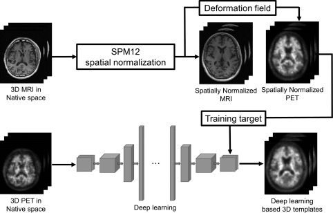
Schematic diagrams of the amyloid PET SN methods compared in this study

2.3. Network architecture

We tested two different deep learning architectures (Figure 2): convolutional auto‐encoder (CAE) and generative adversarial networks (GAN).

Figure 2.

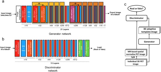
Deep neural network architectures used to generate individually adaptive template for 3D amyloid PET images. (a) CAE, which was also used as the generator in the GAN. (b) Convolutional neural network used as the discriminator in the GAN. (c) Structure of GAN. Each red orange box represents a 3D strided convolutional kernel, where s is the size of the stride and k is the size of the kernels. Each blue box represents batch normalization combined with activation function such as leaky‐ReLU or ELU. The green box shows the fully connected layer with the number of units. The purple box represents the 3D transposed convolutional layer (deconvolution) with two stride and kernel size three. The generator has the architecture of the residual box, as shown in the figure [Color figure can be viewed at http://wileyonlinelibrary.com]

2.3.1. Convolutional auto‐encoder

The detail structure of the CAE is shown in Figure 2a. All convolutional layers extracted the features in a 3D manner. We used strided convolution rather than max‐pooling (Radford, Metz, & Chintala, 2015), and applied the exponential linear unit (ELU) activation function (Clevert, Unterthiner, & Hochreiter, 2015) after the convolution. Batch normalizations were applied except for the final output layer. The input to each block (convolution + ELU + batch normalization) was summed with the output of the block, as suggested by He, Zhang, Ren, and Sun (2015). The input to the CAE was the PET image (344 × 344 × 127) of each individual in native space. The following loss function was minimized while measuring the difference between the output of CAE (91 × 109 × 91) and the MRI‐based SN result to enable CAE to produce the individually adaptive PET template for the SN:

$$L_{{\mathrm{C}\mathrm{A}\mathrm{E}}_{{ }_{ }}}^{ }=\frac{1}{m}\sum _{i=1}^m\frac{{\left(I_i^{\mathrm{M}\mathrm{N}\mathrm{I}}-\mathrm{C}\mathrm{A}\mathrm{E}\left(I_i^{\mathrm{N}\mathrm{a}\mathrm{t}\mathrm{i}\mathrm{v}\mathrm{e}}\right)\right)}^2}{N}$$ (1)

where m is batch size, $I_i^{\mathrm{M}\mathrm{N}\mathrm{I}}$ is the image in MNI space (MRI‐based SN) (label), $I_i^{\mathrm{N}\mathrm{a}\mathrm{t}\mathrm{i}\mathrm{v}\mathrm{e}}$ is the PET image in native space (input), and $N$ is the number of voxels in MNI space.

2.3.2. Modified GAN

The objective of GAN is to produce an image that is similar to the original data distribution. A GAN consists of two networks: generator and discriminator (Goodfellow et al., 2014). The generator, G(·), makes authentic‐looking images and the discriminator, D(·), determines whether the given images are “real” or “fake.” After training both networks, the generator produces authentic‐looking images and the discriminator cannot determine whether the generated images are real or fake. The networks are trained by solving the following min‐max problem:

$$\underset{{\mathrm{\theta }}_{\mathrm{G}}}{\min }\underset{{\mathrm{\theta }}_{\mathrm{D}}}{\max }{\mathbb{E}}_{x\sim p_{\mathrm{d}\mathrm{a}\mathrm{t}\mathrm{a}}\left(x\right)}\left[\log D\left(x\right)\right]+{\mathbb{E}}_{z\sim p_G\left(z\right)}\left[1-\log D\left(G\left(z\right)\right)\right]$$ (2)

where $z$ is the PET image in native space (input), $x$ is the MRI‐based SN result (label), and ${\mathrm{\theta }}_{\mathrm{G}} \mathrm{a}\mathrm{n}\mathrm{d} {\mathrm{\theta }}_{\mathrm{D}}$ are the parameters in the generator and discriminator, respectively. $\mathbb{E}$ stands for the expectation for given probability distribution.

In the original GAN proposed for generation of unsupervised natural looking images, z is a random vector. However, individual PET images in native space are used as input z to the generator in this study. The above equation is solved by alternating the updating of the generator and discriminator. In addition, the fidelity loss between the generated image and the MRI‐based SN result (the label) is added to the GAN min‐max problem to lead the trained generator to produce the template like images as follows:

$$\underset{{\mathrm{\theta }}_{\mathrm{G}}}{\min }\underset{{\mathrm{\theta }}_{\mathrm{D}}}{\max }{\mathbb{E}}_{x\sim p_{\mathrm{d}\mathrm{a}\mathrm{t}\mathrm{a}}\left(x\right)}\left[\log D\left(x\right)\right]+{\mathbb{E}}_{z\sim p_{\mathrm{G}}\left(z\right)}\left[1-\log D\left(G\left(z\right)\right)\right]+{10}^{-5}{L}_{\mathrm{G}\mathrm{A}\mathrm{N}}^{\mathrm{f}\mathrm{i}\mathrm{d}}$$ (3)

where

$$L_{\mathrm{G}\mathrm{A}\mathrm{N}}^{\mathrm{f}\mathrm{i}\mathrm{d}}=\sum _{i=1}^m\frac{{\left(I_i^{\mathrm{M}\mathrm{N}\mathrm{I}}-G\left(z_i\right)\right)}^2}{\sum _{\mathrm{a}\mathrm{l}\mathrm{l} \mathrm{v}\mathrm{o}\mathrm{x}\mathrm{e}\mathrm{l}\mathrm{s}}{I}_i^{\mathrm{M}\mathrm{N}\mathrm{I}}}$$

The guidelines presented by Radford, Metz, and Chintala (2015) were applied to constitute the discriminator. The leaky‐ReLU and strided convolutional layers were used for the discriminator, as shown in Figure 2b.

2.4. Data augmentation and network training

Before the training, PET images were cropped into a 256 × 256 × 106 matrix and down‐sampled to 133 × 133 × 104 to reduce the input data size and to yield the same pixel size as the MNI152 template. The input images and the label data generated by MRI‐based SN were rescaled to [–1, 1]. The training set was augmented by rotating the images in 3D orthogonal planes with different orientations each iteration. The rotation angles around the three axes were randomly selected from [–8°, 8°]. Accordingly, the total pieces of data in the training set was 527 (subject) × 1300 (epoch) = 685,100.

The number of epochs, batch size, and initial learning rate were 1300, 5, and 0.007, respectively. The learning rate decayed by a factor of 0.1 every 420 epochs. The loss function was minimized using the adaptive moment estimation method with ${\mathrm{\beta }}_{1 }$= 0.5 (Kingma & Ba, 2014). Gaussian noise of 0.2 standard deviation was added to the inputs for discriminator to stabilize the training of the GAN (Sønderby, Caballero, Theis, Shi, & Huszár, 2016). Our implementation is based on TensorFlow, NVIDIA GeForce 1080 GPU, and Intel i7–7700K CPU.

2.5. Image analysis

To compare the different SN methods, MRI‐based, DL‐based, and average template‐based ones, we calculated the regional activity concentration of ¹¹C‐PIB (kBq/mL) in eight brain regions (frontal, temporal, parietal, occipital, cingulate cortex, striatum, thalamus, and cerebellum) in each hemisphere using the Automated Anatomical Labeling atlas. The standardized uptake value ratio (SUVr) was also obtained by normalizing the activity concentration of each region to that of the cerebellum. The correlation between PET‐ and MRI‐based SN was assessed using Pearson's correlation on the regional activity concentration and SUVr. We also performed Bland‐Altman analysis on the regional activity concentration and SUVr.

In addition, SUVr images were smoothed with a Gaussian filter at 8‐mm full width at half maximum for voxel‐wise comparisons. Voxel‐wise analysis of SUVr images was then performed by one‐way analysis of variance (ANOVA) among the different SN methods. Additionally, SUVr images were compared among CN, MCI, and AD groups for each SN approach to assess how each SN approach can detect differential uptake patterns according to clinical status. Thresholds of p < .05 corrected for a family wise error and k > 100 contiguous voxels were applied.

3. RESULTS

The loss functions of CAE and modified GAN maintained a steady curve after ∼45,000 iterations (total number of iterations = 90,000). The time taken to train the networks was ∼30 and 48 hr for CAE and GAN, respectively. After the training, both the CAE and modified GAN successfully generated adaptive amyloid PET templates as shown in Figures 3 and 4. In both amyloid negative (Figure 3) and positive (Figure 4) test dataset, the DL‐generated PET templates (a and b) were quite different from the average PET template (c) but similar to the MRI‐based SN result (d), as intended (in training). No discontinuity of brain and other structures was observed in any of the three orthogonal planes because our deep learning networks processed the 3D volume.

Figure 3.

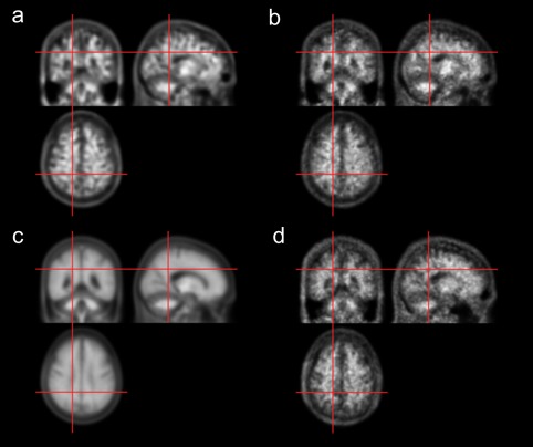
¹¹C‐PIB PET templates generated using deep neural networks for an amyloid negative case. (a) CAE‐generated template. (b) GAN‐generated template. (c) Average template. (d) Spatially normalized image using MRI, which serves as the label for CAE and GAN training [Color figure can be viewed at http://wileyonlinelibrary.com]

Figure 4.

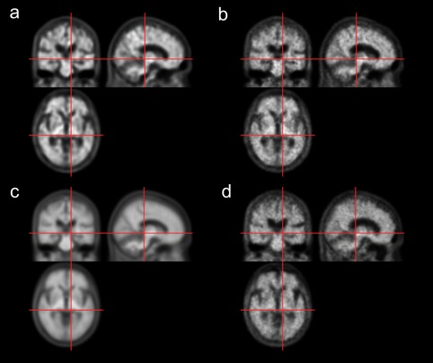
¹¹C‐PIB PET templates generated using deep neural networks for an amyloid positive case. (a) CAE‐generated template. (b) GAN‐generated template. (c) Average template. (d) Spatially normalized image using MRI, which serves as the label for CAE and GAN training [Color figure can be viewed at http://wileyonlinelibrary.com]

Figure 5 shows the spatially normalized PET images for the CAE‐ and GAN‐generated PET templates (a and b) and the average PET template (c). The images spatially normalized using the DL‐based approaches show an amyloid uptake pattern that is very similar to the MRI‐based SN result shown in Figure 5d. However, the average PET template led to a different uptake pattern, as indicated in Figure 5c by the white arrows and circle.

Figure 5.

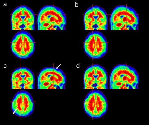
Results of SN of a representative ¹¹C‐PIB PET image onto (a) CAE‐generated, (b) GAN‐generated, and (c) average PET templates. (d) Spatially normalized image using MRI [Color figure can be viewed at http://wileyonlinelibrary.com]

The superiority of the deep learning approach is more remarkable in the quantitative analysis. The Figure 6 shows the mutual information and mean squared error between the spatially normalized PET images with and without the help of MRI. Figure 7 shows the scattered plot with regression line and Bland‐Altman plot between the regional activity concentration obtained from the spatially normalized PET images with and without the help of MRI. The regional activity concentration (kBq/mL) of ¹¹C‐PIB, obtained from the spatially normalized image onto the average PET template, were underestimated relative to those from the MRI‐based SN result (Figure 7c). In contrast, both the CAE and GAN yield unbiased results with better correlation, as shown in Figure 7a,b. The superiority of the deep learning approach is more remarkable in the same analysis on the regional SUVr estimation (Figure 8).

Figure 6.

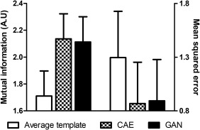
The mutual information and mean squared error between the spatially normalized PET images with and without the help of MRI

Figure 7.

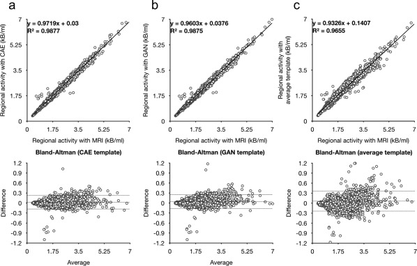
Scattered and Bland‐Altman plots between regional activity concentration estimated from the results of MRI‐based SN and different PET‐based approaches using (a) CAE‐generated, (b) GAN‐generated, and (c) average ¹¹C‐PIB PET templates

Figure 8.

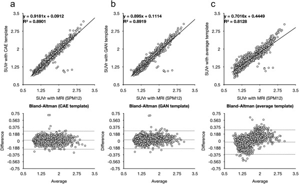
Scattered and Bland‐Altman plots between SUVr estimated from the results of MRI‐based SN and different PET‐based approaches using (a) CAE‐generated, (b) GAN‐generated, and (c) average ¹¹C‐PIB PET templates

The Figure 9 shows the results of voxel‐wise comparisons of SUVr images spatially normalized with the help of MRI and PET‐based approaches using (a) average ¹¹C‐PIB PET template, (b) CAE‐generated PET template, and (c) GAN‐generated PET template. Mainly in the boundaries among gray matter and white matter and cerebral fluid space, the average PET template yielded significant SUVr difference that was reduced by use of CAE‐ and GAN‐generated templates. In addition, the deep learning approaches were as sensitive as the MRI‐based SN in group comparison of SUVr. However, the average PET template approach led to the sensitivity decrease (Figure 10).

Figure 9.

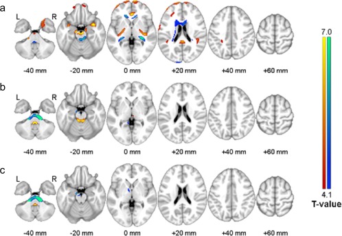
Voxel‐wise comparisons of SUVr images spatially normalized with the help of MRI and PET‐based approaches using (a) average 11C‐PIB PET template, (b) CAE‐generated PET template, and (c) GAN‐generated PET template. Red indicates regions with overestimated SUVr using the PET‐based approach, and blue with underestimated SUVr, compared with the approach with the help of MRI [Color figure can be viewed at http://wileyonlinelibrary.com]

Figure 10.

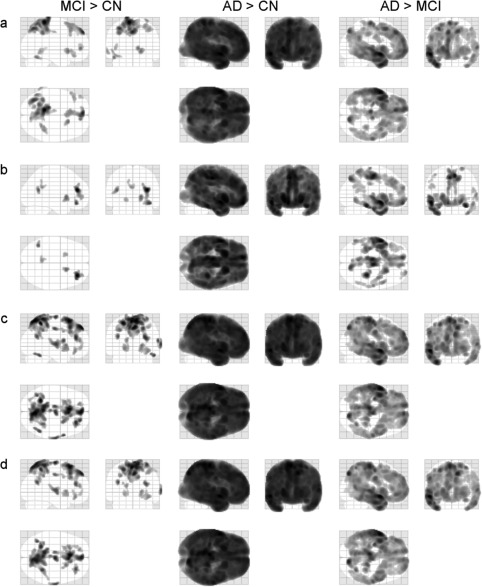
Glass brain images of regions with increased SUVr in MCI and AD groups using (a) MRI‐based SN template, (b) average 11C‐PIB template, (c) CAE‐generated PET template, and (d) GAN‐generated PET template

The time spent generating a template image using the trained deep learning networks was ∼0.02 s.

4. DISCUSSION

Although deep learning is showing great potential in the medical imaging field, applying natural image processing deep learning algorithms successfully to medical images is not straightforward. Natural images and medical images have different characteristics in many aspects. For example, the pixel intensity of PET images has more quantitative information (i.e., kBq/mL) than that of natural images. Usually, a much smaller quantity of data is available for training the networks in medical imaging than in natural imaging. Further, the ground truth of labeled data for supervised learning is unknown or suboptimal in many medical imaging problems such as the SN of brain images. Most natural image processing techniques are applied to 2D images, whereas 3D or higher dimensional data have to be handled in medical image processing and analysis. In SN of brain images, the brain deformations are processed using 3D fields.

In this study, we trained deep neural networks to produce an individually adaptive PET template when an amyloid PET image is given to the networks as input. The training network was supervised using the MRI‐based SN result as the label of the networks. The output of the trained network was ultimately used as the template for SN of amyloid PET without use of matched 3D MRI. The DL‐based PET templates resulted in significantly better correlation and bias properties than the average templates, as shown in Figures 7 and 8, when the MRI‐based SN results were regarded as ground truth.

A potential problem with CAE is blurred output images that results in loss of the anatomical detail of brain structures. An approach that has gained significant popularity for preserving the structural detail in output image is U‐net. In U‐net, the front layers in the contraction pathway are combined with the back layers in the expansion pathway. However, the U‐net structure is not appropriate in our SN problem because U‐net requires same dimension and shape for both the input and output. Alternatively, we tested GAN with the additional fidelity loss function presented in Equation (3). In our preliminary studies, the GAN without the fidelity loss function could not produce relevant output images similar to the input or label data. In addition, the anatomical details shown in the CAE‐ and GAN‐generated templates were not significantly different, although the noise level was lower in the CAE‐generated one (Figures 3 and 4). These results imply that the measurement of fidelity loss is important in this specific task for generating individualized amyloid PET templates based on deep learning.

Recently, Choi and Lee (in press) proposed a GAN‐based approach for virtual MRI generation from the ¹⁸F‐florbetapir PET for the same purpose as this study. They performed the SN of GAN‐generated MRI onto the MRI template and applied the obtained SN parameter to the input PET image. This method also outperformed the conventional SN strategies without use of MRI. However, the generation of individualized PET templates in standard coordinates as suggested in the present study would be more relevant in many other applications because the current approach does not require transmodal transition of images (from PET to MRI). Deep learning‐based trans‐modal transition is gaining increased attention (i.e., virtual CT from MR images; Han, 2017; Nie, Cao, Gao, Wang, & Shen, 2016). In these applications, the deep learning networks can generate output images that look similar to the label. However, if there is no physically or physiologically relevant underlying principles that can explain the transition mechanism completely or partially, such trans‐modal transitions can lead to unexpected errors.

5. CONCLUSIONS

In this study, we developed a deep neural networks‐based approach for generating adaptive PET templates for robust and accurate MRI‐less SN of ¹¹C‐PIB PET. The proposed deep learning approach significantly enhances the quantitative accuracy of MRI‐less amyloid PET assessment by reducing the SN error observed when an average amyloid PET template was used. The trained deep neural networks provide adaptive 3D PET templates without any discontinuity between the slices very quickly (0.02 s) once the input image is given. Because the proposed method does not require 3D MR images for the SN of PET images, it has great potential for use in routine analysis of amyloid PET images for clinical practice and research.

Kang SK, Seo S, Shin SA, et al. Adaptive template generation for amyloid PET using a deep learning approach. Hum Brain Mapp. 2018;39:3769–3778. 10.1002/hbm.24210

REFERENCES

- An, H. J. , Seo, S. , Kang, H. , Choi, H. , Cheon, G. J. , Kim, H.‐J. , … Lee, J. S. (2016). MRI‐based attenuation correction for PET/MRI using multiphase level‐set method. Journal of Nuclear Medicine, 57(4), 587–593. [DOI] [PubMed] [Google Scholar]
- Ashburner, J. , & Friston, K. J. (1999). Nonlinear spatial normalization using basis functions. Human Brain Mapping, 7(4), 254–266. [DOI] [PMC free article] [PubMed] [Google Scholar]
- Ashburner, J. , & Friston, K. J. (2005). Unified segmentation. Neuroimage, 26(3), 839–851. [DOI] [PubMed] [Google Scholar]
- Avants, B. B. , Tustison, N. J. , Song, G. , Cook, P. A. , Klein, A. , & Gee, J. C. (2011). A reproducible evaluation of ANTs similarity metric performance in brain image registration. Neuroimage, 54(3), 2033–2044. [DOI] [PMC free article] [PubMed] [Google Scholar]
- Barthel, H. , Gertz, H.‐J. , Dresel, S. , Peters, O. , Bartenstein, P. , Buerger, K. , … Reininger, C. (2011). Cerebral amyloid‐β PET with florbetaben (18 F) in patients with Alzheimer's disease and healthy controls: A multicentre phase 2 diagnostic study. The Lancet Neurology, 10(5), 424–435. [DOI] [PubMed] [Google Scholar]
- Brett, M. , Christoff, K. , Cusack, R. , & Lancaster, J. (2001). Using the Talairach atlas with the MNI template. Neuroimage, 13(6), 85. [Google Scholar]
- Choi, H. , & Lee, D. S. Generation of structural MR images from amyloid PET: Application to MR‐less quantification. Journal of Nuclear Medicine, In press, doi: 10.2967/jnumed.117.199414 [DOI] [PMC free article] [PubMed] [Google Scholar]
- Ciresan, D. , Giusti, A. , Gambardella, L. M. , & Schmidhuber, J. (2012). Deep neural networks segment neuronal membranes in electron microscopy images. Advances in Neural Information Processing Systems, 2843–2851. [Google Scholar]
- Clevert, D.‐A. , Unterthiner, T. , & Hochreiter, S. (2015). Fast and accurate deep network learning by exponential linear units (ELUs). arXiv, 1511.07289. [Google Scholar]
- Dey, D. , Chaudhuri, S. , & Munshi, S. (2018). Obstructive sleep apnoea detection using convolutional neural network based deep learning framework. Biomedical Engineering Letters, 8(1), 95–100. [DOI] [PMC free article] [PubMed] [Google Scholar]
- Evans, A. C. , Janke, A. L. , Collins, D. L. , & Baillet, S. (2012). Brain templates and atlases. Neuroimage, 62(2), 911–922. [DOI] [PubMed] [Google Scholar]
- Goodfellow, I. J. , Pouget‐Abadie, J. , Mirza, M. , Xu, B. , Warde‐Farley, D. , Ozair, S. , … Bengio, Y. (2014). Generative Adversarial Networks. arXiv, 1406.2661. [Google Scholar]
- Han, X. (2017). MR‐based synthetic CT generation using a deep convolutional neural network method. Medical Physics, 44(4), 1408–1419. [DOI] [PubMed] [Google Scholar]
- He, K. , Zhang, X. , Ren, S. , & Sun, J. (2015). Deep Residual Learning for Image Recognition. arXiv, 1512.03385. [Google Scholar]
- Hwang, D. , Kim, K. Y. , Kang, S. K. , Seo, S. , Paeng, J. C. , Lee, D. S. , & Lee, J. S. Improving accuracy of simultaneously reconstructed activity and attenuation maps using deep learning. Journal of Nuclear Medicine, In press, doi: 10.2967/jnumed.117.202317 [DOI] [PubMed] [Google Scholar]
- Kang, K. W. , Lee, D. S. , Cho, J. H. , Lee, J. S. , Yeo, J. S. , Lee, S. K. , … Lee, M. C. (2001). Quantification of F‐18 FDG PET images in temporal lobe epilepsy patients using probabilistic brain atlas. Neuroimage, 14(1), 1–6. [DOI] [PubMed] [Google Scholar]
- Kingma, D. , & Ba, J. (2014). Adam: A method for stochastic optimization. arXiv Preprint, arXiv, 1412.6980. [Google Scholar]
- Klein, A. , Andersson, J. , Ardekani, B. A. , Ashburner, J. , Avants, B. , Chiang, M.‐C. , … Hellier, P. (2009). Evaluation of 14 nonlinear deformation algorithms applied to human brain MRI registration. Neuroimage, 46(3), 786–802. [DOI] [PMC free article] [PubMed] [Google Scholar]
- Klunk, W. E. , Engler, H. , Nordberg, A. , Wang, Y. , Blomqvist, G. , Holt, D. P. , … Estrada, S. (2004). Imaging brain amyloid in Alzheimer's disease with Pittsburgh Compound‐B. Annals of Neurology, 55(3), 306–319. [DOI] [PubMed] [Google Scholar]
- Krizhevsky, A. , Sutskever, I. , & Hinton, G. E. (2012). Imagenet classification with deep convolutional neural networks. Advances in Neural Information Processing Systems, 1097–1105. [Google Scholar]
- Lancaster, J. L. , Glass, T. G. , Lankipalli, B. R. , Downs, H. , Mayberg, H. , & Fox, P. T. (1995). A modality‐independent approach to spatial normalization of tomographic images of the human brain. Human Brain Mapping, 3(3), 209–223. [Google Scholar]
- Lee, D. Y. , Choo, I. H. , Jhoo, J. H. , Kim, K. W. , Youn, J. C. , Lee, D. S. , … Woo, J. I. (2006). Frontal dysfunction underlies depressive syndrome in Alzheimer disease: a FDG‐PET study. The American Journal of Geriatric Psychiatry, 14, 625–628. [DOI] [PubMed] [Google Scholar]
- Lee, J. S. , Kim, B. N. , Kang, E. , Lee, D. S. , Kim, Y. K. , Chung, J. K. , … Cho, S. C. (2005). Regional cerebral blood flow in children with attention deficit hyperactivity disorder: Comparison before and after methylphenidate treatment. Human Brain Mapping, 24(3), 157–164. [DOI] [PMC free article] [PubMed] [Google Scholar]
- Lee, J. S. , Lee, D. S. , Kim, S.‐K. , Lee, S.‐K. , Chung, J.‐K. , Lee, M. C. , & Park, K. S. (2000). Localization of epileptogenic zones in F‐18 FDG brain PET of patients with temporal lobe epilepsy using artificial neural network. IEEE Transactions on Medical Imaging, 19, 347–355. [DOI] [PubMed] [Google Scholar]
- Leynes, A. P. , Yang, J. , Wiesinger, F. , Kaushik, S. S. , Shanbhag, D. D. , Seo, Y. , … Larson, P. E. (2018). Zero Echo‐time and Dixon Deep pseudoCT (ZeDD‐CT): Direct PseudoCT Generation for Pelvis PET/MRI Attenuation Correction using Deep Convolutional Neural Networks with Multi‐parametric MRI. Journal of Nuclear Medicine, 59(5), 852–858. 10.2967/jnumed.117.198051 [DOI] [PMC free article] [PubMed] [Google Scholar]
- Long, J. , Shelhamer, E. , & Darrell, T. (2015). Fully convolutional networks for semantic segmentation, Proceedings of the IEEE conference on Computer Vision and Pattern Recognition, 3431–3440. [DOI] [PubMed]
- Mansour, R. F. (2018). Deep‐learning‐based automatic computer‐aided diagnosis system for diabetic retinopathy. Biomedical Engineering Letters, 8(1), 41–57. [DOI] [PMC free article] [PubMed] [Google Scholar]
- Minoshima, S. , Frey, K. A. , Koeppe, R. A. , Foster, N. L. , & Kuhl, D. E. (1995). A diagnostic approach in Alzheimer's disease using three‐dimensional stereotactic surface projections of fluorine‐18‐FDG PET. Journal of Nuclear Medicine, 36, 1238–1248. [PubMed] [Google Scholar]
- Minoshima, S. , Koeppe, R. A. , Frey, K. A. , & Kuhl, D. E. (1994). Anatomic standardization: Linear scaling and nonlinear warping of functional brain images. Journal of Nuclear Medicine, 35, 1528–1537. [PubMed] [Google Scholar]
- Nie, D. , Cao, X. , Gao, Y. , Wang, L. , & Shen, D. (2016). Estimating CT Image from MRI Data Using 3D Fully Convolutional Networks, Deep learning and data labeling for medical applications: First International Workshop, LABELS 2016, and second International Workshop, DLMIA 2016, held in conjunction with MICCAI 2016, Athens, Greece, October 21, 170–178. [DOI] [PMC free article] [PubMed] [Google Scholar]
- Radford, A. , Metz, L. , & Chintala, S. (2015). Unsupervised Representation Learning with Deep Convolutional Generative Adversarial Networks. arXiv Preprint, arXiv, 1511.06434. [Google Scholar]
- Simonyan, K. , & Zisserman, A. (2014). Very deep convolutional networks for large‐scale image recognition. arXiv Preprint, arXiv, 1409.1556. [Google Scholar]
- Suk, H.‐I. , Lee, S.‐W. , & Shen, D. & Alzheimers Disease Neuroimaging Initiative (2014). Hierarchical feature representation and multimodal fusion with deep learning for AD/MCI diagnosis. Neuroimage, 101, 569–582. [DOI] [PMC free article] [PubMed] [Google Scholar]
- Sønderby, C. K. , Caballero, J. , Theis, L. , Shi, W. , & Huszár, F. (2016). Amortised MAP Inference for Image Super‐resolution. arXiv, 1610.04490. [Google Scholar]
- Xie, J. , Xu, L. , & Chen, E. (2012). Image denoising and inpainting with deep neural networks. Advances in Neural Information Processing Systems, 341–349. [Google Scholar]