

Abstract
Objectives: Tissue microstructure features, namely axon radius and volume fraction, provide important information on the function of white matter pathways. These parameters vary on the scale much smaller than imaging voxels (microscale) yet influence the magnetic resonance imaging diffusion signal at the image voxel scale (macroscale) in an anomalous manner. Researchers have already mapped anomalous diffusion parameters from magnetic resonance imaging data, but macroscopic variations have not been related to microscale influences. With the aid of a tissue model, we aimed to connect anomalous diffusion parameters to axon radius and volume fraction using diffusion‐weighted magnetic resonance imaging measurements. Experimental design: An ex vivo human brain experiment was performed to directly validate axon radius and volume fraction measurements in the human brain. These findings were validated using electron microscopy. Additionally, we performed an in vivo study on nine healthy participants to map axon radius and volume fraction along different regions of the corpus callosum projecting into various cortical areas identified using tractography. Principal observations: We found a clear relationship between anomalous diffusion parameters and axon radius and volume fraction. We were also able to map accurately the trend in axon radius along the corpus callosum, and in vivo findings resembled the low‐high‐low‐high behaviour in axon radius demonstrated previously. Conclusions: Axon radius and volume fraction measurements can potentially be used in brain connectivity studies and to understand the implications of white matter structure in brain diseases and disorders. Hum Brain Mapp 38:1068–1081, 2017. © 2016 Wiley Periodicals, Inc.
Keywords: magnetic resonance imaging, anomalous diffusion, microstructure, corpus callosum, axon radius, volume fraction
Abbreviations
- DW‐MRI
diffusion‐weighted magnetic resonance imaging
INTRODUCTION
Maps of axon radius and volume fraction provide information on the characteristics of white‐matter pathways that significantly influence their function [Aboitiz et al., 1992; Alexander et al., 2010; Assaf et al., 2004]. Axon radius influences nerve conduction velocity, affecting the speed and synchronization of neural processing [Hursh 1939; Ritchie 1982; Tomasi et al., 2012; Waxman 1980]. For example, large diameter axons in the corpus callosum mediate rapid interhemispheric information transfer, allowing the coordination of specialised hemispheric activities [Aboitiz et al., 1992; Ringo et al., 1994]. Maps of axon radius and axon volume fraction may also yield tissue biomarkers in neurological disorders and it has been hypothesized that the axon radius distribution in the corpus callosum is altered in amyotrophic lateral sclerosis [Cluskey and Ramsden, 2001; Heads et al., 1991], dyslexia [Njiokiktjien et al., 1994], schizophrenia [Randall, 1983; Rice and Barone, 2000], and autism [Hughes, 2007; Piven et al., 1997].
Research on animals and humans has focused on extracting information on axon radius and volume fraction from diffusion‐weighted magnetic resonance imaging (DW‐MRI) data with the aid of tissue models [Alexander, 2008; Alexander et al., 2010; Assaf et al., 2004; Assaf et al., 2008; Barazany et al., 2009; Ong et al., 2008; Panagiotaki et al., 2012; Yablonskiy and Sukstanskii, 2010; Zhang et al., 2011]. The models assume that axonal structure is cylindrical, fibres are highly oriented and axon radii follow a gamma distribution. Properties associated with axons are inferred from measurements of water diffusion and the acquired signal is modelled in terms of compartments corresponding to tissue components with different diffusion characteristics. Water movement within image voxels can be restricted (intra‐axonal) or hindered (extra‐axonal). The restricted compartment plays an essential role in the estimation of axon radius. To date it has been assumed that in this compartment the mean‐squared displacement of water diffusion remains Gaussian during the gradient field applied to sensitise individual measurements. However, during DW‐MRI measurements, diffusion takes place on a time scale within which boundary and interface interactions can occur, and the Gaussian mean‐squared displacement assumption does not hold.
In practice, measurement times with DW‐MRI lie between 10 ms and 100 ms [Mori and Zhang, 2006; Yablonskiy and Sukstanskii, 2010]. These times correspond to a root mean‐squared displacement of water diffusion of around 5.8 µm to 18.4 µm when diffusivity (D) is approximately 1.7 µm2/ms. Hence, water molecules diffusing within axons up to 5 µm in radius, which are common in the normal human brain [Aboitiz et al., 1992], have a high chance of encountering boundaries. Diffusion within the time regime may be anomalous [Price, 2009] because the measured DW‐MRI signal at the voxel level may not be strictly governed by Brownian motion. As a consequence, mean squared displacement of water diffusion shifts away from the Gaussian distribution [Sen, 2003; Upadhyaya et al., 2001]. Although tissue compartments with restricted and hindered diffusion are recognised in existing models [Alexander, 2008; Alexander et al., 2010; Assaf et al., 2004; Assaf et al., 2008; Barazany et al., 2009; Ong et al., 2008; Panagiotaki et al., 2012; Yablonskiy and Sukstanskii, 2010; Zhang et al., 2011], DW‐MRI signal models incorporating anomalous diffusion have not been systematically studied for the purpose of resolving the distribution of axon radii and axonal volume fraction [Alexander, 2008; Alexander et al., 2010; Assaf et al., 2004; Assaf et al., 2008; Barazany et al., 2009; Dyrby et al., 2013; Zhang et al., 2011].
The solution to the classical Bloch‐Torrey equation describing diffusion measured with MRI assumes Gaussian diffusion [Abragam, 2002; Donskaya, 1973; Kaplan, 1959; Rohmer and Gullberg, 2006; Torrey, 1956] and does not naturally lend itself to the exploration of anomalous dynamics in MRI. In the fields of physics, chemistry and engineering, the use of the continuous time random walk (CTRW) theory [Metzler and Klafter, 2000; Metzler and Klafter, 2004] has led to specific methods catering for anomalous dynamics [Bouchaud and Georges, 1990; Gorenflo et al., 2002; Hilfer, 2000; Hughes, 1995; Klafter et al., 1996; Shlesinger et al., 1993; Yu et al., 2008; Zaslavsky, 2002]. Classical Brownian motion theory was extended by generalizing the Gaussian probability density function for situations where a mismatch between the scale at which measurements are taken and the scale at which changes occur is present. Fractional calculus (calculus using non‐integer derivatives) provides a mechanistic approach for formulating equations for such systems and equations representing anomalous diffusion have been developed using non‐integer derivatives [Khanafer et al., 2003; Magin et al., 2008; Norris, 2001] allowing anomalous dynamics in MRI to be characterised [Ingo et al., 2015; Kimmich, 2002; Köpf et al., 1998; Liang et al., 2016; Magin et al., 2009; Magin et al., 2013; Magin et al., 2011; Stapf et al., 1995; Stapf, 2002].
Several CTRW models [Ingo et al., 2015; Magin et al., 2013] and a fractal derivative diffusion model [Liang et al., 2016] have been proposed to characterise anomalous diffusion in DW‐MRI for the purpose of studying the microstructure of biological tissue. The parameters of the CTRW model provided exquisite grey‐white matter contrast and the parameters were stated to be linked to sub‐ and super‐diffusion [Ingo et al., 2015; Magin et al., 2013]. A fractional derivative model based on fractal time and space derivatives has also been considered to fit diffusion‐weighted imaging data as a means of relating sub‐voxel level tissue composition to MRI diffusion signal behaviour [Liang et al., 2016]. The model was based on Fick's second law of diffusion. Spectral entropy, a model parameter, was found to be a quantitative measure of tissue complexity and heterogeneity and showed good separation between grey and white matter. The fractal model did not fit the data as well as the CTRW model, perhaps reflecting the basis of the fractal model in Fick's second law of diffusion as opposed to the Bloch‐Torrey equation which is the basis of the CTRW model and is more relevant in the MRI context. The CTRW model is fractional in both time and space.
For the purpose of estimating axon radius and volume fraction based on anomalous diffusion, we considered anomalous diffusion in space. This is because water diffusion is assumed to be restricted or hindered by spatial structures, such as the axonal wall. This was represented using a previously described three parameter space‐fractional Bloch‐Torrey model [Magin et al., 2008]. A white matter tissue model incorporating four tissue compartments with different diffusion profiles was used [Alexander et al., 2010]: intra‐axonal space (ia) corresponding to the compartment with restricted diffusion, extra‐axonal space corresponding to the compartment with hindered diffusion (hd), cerebrospinal fluid (csf) and trapped water (tw). The tissue model was used to produce synthetic maps of the three anomalous diffusion equation parameters as a function of axon radius and volume fraction. Experimental data were fitted using the anomalous diffusion equation and, axon radius and volume fraction were deduced by matching experimentally measured parameters to values in the synthetic parameter maps. We compared axon radius and volume fraction estimates obtained using anomalous diffusion in ex vivo and in vivo ultra‐high field DW‐MRI data with measurements made using ex vivo electron microscopy of the corpus callosum (see Fig. 1A), as it is known that white matter projections into various cortical regions (locations 1 to 7 in Fig. 1B) have different axon radii [Caminiti et al., 2009, 2013Tomasi et al., 2012] and volume fractions.
Figure 1.
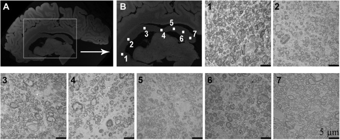
Ex vivo structural brain magnetic resonance images in the sagittal orientation showing the target region used in our study. (A) Ex vivo structural image showing the location of the corpus callosum. (B) Enlargement of the corpus callosum showing seven distinct locations along the corpus callosum used in the assessment of axon radius and volume fraction. Axon radius and volume fraction is known to vary along the locations shown in the corpus callosum. A representative electron microscopy image for each location is provided as well.
MATERIALS AND METHODS
Background on Anomalous Diffusion
A number of studies have focused on the treatment of non‐Gaussian diffusion. Numerous authors have reported that non‐Gaussian models, namely the bi‐exponential and stretched exponential models, improve the fitting of diffusion data [Hall and Barrick, 2008; Khanafer et al., 2003; Norris, 2001; Speck et al., 2001]. These methods have not been evaluated and validated in detail, which is likely due to a lack of in‐depth problem formulation and associated numerical methods of solution. Recently, fractional order calculus was used to investigate the link between fractional order dynamics and diffusion by solving the space and time fractional Bloch‐Torrey equation (ST‐FBTE) [Magin et al., 2008; Yu et al., 2012; Yu et al., 2013a; Yu et al., 2013b; Zhou et al., 2010]
| (1) |
where , i is the complex identity, , is the gyromagnetic ratio, G(t) and D are the magnetic field gradient and the diffusion coefficient, respectively. is the Caputo time fractional derivative of order , is a sequential Riesz fractional order operator in space [Kilbas et al., 2006]. In addition, comprises the transverse components of the magnetization; and are the fractional order time and space constants needed to preserve units, and in (0, 1] and in (0.5, 1]. Magin et al. solved the fractional governing equations in space ( and ) and time ( and ) separately [Magin et al., 2008]. They investigated the solution obtained from the space fractional Bloch‐Torrey equation with the Stejskal‐Tanner gradient:
| (2) |
We developed numerical approaches of solving ST‐FBTE and proved the stability and convergence of the methods [Yu et al., 2012; Yu et al., 2013a, 2013b]. Equation (2) was used to fit diffusion‐weighted images acquired for a normal human brain [Magin et al., 2008]. This allowed construction of D, and maps. However, they did not evaluate changes with respect to changes in the micro‐environment, especially how to biophysically interpret the meaning of and . In a follow‐up study by the same group, Zhou et al. used (2) to analyse diffusion images of healthy human brain in vivo extending their work to high b‐values up to 4,700 s/mm2 in five healthy volunteers [Zhou et al., 2010]. They also demonstrated that the twice‐refocused spin echo diffusion sequence can be used to acquire the data used in the fitting [Gao et al., 2011]. Both Zhou et al. and Hall and Barrick stated that further studies are needed to understand the influence of tissue microstructure on the anomalous diffusion parameters.
Tissue Model
The model of water diffusion in white matter proposed by Alexander et al. [2010] has four signal compartments, denoted as S ia, S hd, S csf, and S tw, each contributing to the MRI signal of an image voxel.
S ia: Intra‐axonal restricted diffusion represented by cylinders following the Gaussian phase distribution approximation. When the echo time is much longer than the gradient pulse duration [van Gelderen et al., 1994], the signal is represent as:
| (3) |
where is the MRI signal without diffusion weighting, is the gradient duration, and R is the representative intra‐axonal radius.
Shd: Hindered diffusion in extra‐axonal space following anisotropic Gaussian distributed displacements [Basser et al., 1994]. The compartment signal is [Alexander, 2008; Alexander et al., 2010]:
| (4) |
where , in the MRI context referred to as the b‐value, where is the time between the two pulses. wherein d is the gradient direction d = (d 1, d 2, d 3)T, and n is the vector representing fibre direction, D ∥ is the diffusivity along n, D ⊥ is the apparent diffusivity perpendicular to n, and I is the three dimensional identity matrix. The intrinsic diffusivity inside the cylinders for model S ia is the same as D ∥. Szafer et al. proposed a simple tortuosity model [Szafer et al., 1995]:
| (5) |
where v = f ia/(f ia + f hd) and f ia and f hd are the volume fractions of S ia and S hd.
Scsf: The partial volume effect due to CSF governed by isotropic Gaussian displacements [Barazany et al., 2009]:
| (6) |
where D csf = 3 µm2/ms representing diffusion in the CSF.
Stw: Stationary water from subcellular structures, which is not attenuated by the diffusion weighting [Alexander et al., 2010]:
| (7) |
With the above four compartments, and assuming water molecule exchange does not occur between compartments [Alexander et al., 2010], the total diffusion MRI signal is:
| (8) |
where f represents volume fractions, and .
Data Acquisition
Both the ex vivo and in vivo studies were approved by the University of Queensland's Human Research Ethics Committee, Brisbane, Australia. Participants provided written consent prior to participating in the study. All datasets were de‐identified prior to processing.
Ex vivo human brain study
Human data
One hemisphere of a 60 year old male human brain fixed in 4% paraformaldehyde in phosphate buffered saline was obtained from the Queensland Brain Bank. Sagittal brain sections of around 2 mm thickness were sectioned approximately 5 mm from the midline. The corpus callosum was surgically removed and using a guillotine blade. Seven 1 mm by 1 mm by 2 mm (into the section) tissue specimens were cut (see Fig. 1B for specific locations). These were mounted to a NMR tube using ethyl cyanoacrylate (i.e., superglue), separated by approximately 2‐3 mm each. The tube was then filled with saline. The tube was left for one day, and then saline was replaced with fresh saline. This process was repeated over a period of four days to remove excess paraformaldehyde, which is known to shorten MRI relaxation times and adversely affect imaging due to a lack of signal. MRI data was collected on a 7T Bruker Clinscan research animal scanner. A standard localiser was used to adjust the field‐of‐view of imaging for the diffusion scan. The following parameters of a twice refocused spin echo (2D EPI‐DWI sequence) based diffusion‐weighted imaging sequence were used to acquire the ex vivo MRI data: TE/TR = 49/10,000 ms, Matrix = 40 by 136, bandwidth = 2,828 Hz/pixel, flip angle = 90°, and one single slice with a 400 micron isotropic resolution. Gradient pulse duration = 11.21 ms and separation = 17.41 ms, number of averages = 1, and slice thickness = 0.4 mm. Eleven b‐values between 0 and 5,000 s/mm2 in steps of 500 s/mm2 were acquired and the signal‐to‐noise ratio was maintained across all b‐values (i.e., number of diffusion directions, as specified in Table 1, increased with b‐value and diffusion gradient directions were derived using the electrostatic model). MRtrix was used to calculate axial diffusivity at b‐value = 1,500 s/mm2.
Table 1.
The number of diffusion directions acquired for each b‐value in ex vivo and in vivo study
| b‐value (s/mm2) | 500 | 1,000 | 1,500 | 2,000 | 2,500 | 3,000 | 3,500 | 4,000 | 4,500 | 5,000 |
|---|---|---|---|---|---|---|---|---|---|---|
| Number of diffusion directions | 3 | 3 | 6 | 6 | 9 | 12 | 15 | 18 | 21 | 24 |
Two zero b‐value images were acquired in the case of the ex vivo experiment, and only a single zero b‐value was acquired for the in vivo experiment
Electron microscopy
Seven ex vivo specimens at location shown in Fig. 1B were used for validation based on electron microscopy findings using established methods [Bozzola and Russell, 1999; Braitenberg and Schüz, 1998; Dykstra and Reuss, 2003]. After the ex vivo MRI scan, samples were fixed in 2.5% glutaraldehyde in phosphate buffered saline and stored in this solution at 4°C until subsequent processing. They were washed in phosphate buffered saline and then postfixed in 0.1% osmium tetroxide with the assistance of a PelcoBiowave microwave oven as were all subsequent processing steps. The samples were washed in a graded series of acetone and infiltrated with Epon resin. The resin was polymerised at 60°C over 2 days. Semi‐thin sections of 500 nm thickness were cut, mounted on glass slides and stained with 1% toluidine blue. Thin sections of 50–60 nm were also cut from these resin blocks using a Leica Ultracut S ultramicrotome and picked up on copper grids. They were stained with 5% uranyl acetate in 50% ethanol and Reynold's lead citrate before being observed in a JEOL 1010 transmission electron microscope operated at 80 kV. Images were collected using an Olympus‐Soft Imaging Veleta digital camera.
Steps for processing electron microscopy data
Electron microscopy was performed to do histological analysis [Bozzola and Russell, 1999; Braitenberg and Schüz, 1998; Dykstra and Reuss, 2003]. The corpus callosum was isolated and we marked seven locations (see Fig. 1B) and took five histological specimens from each. A representative electron microscopy image for each location is also provided in Fig. 1.
ImageJ, a software package for quantitative image analysis, was used to calculate axon radii and volume fraction from the electron microscopy images. A region‐of‐interest of size 20 × 20 µm2 was chosen within each image. After manually adjusting the threshold parameters in ImageJ to delineate myelination, the axons were selected (see Fig. 2) from five images at each location within the corpus callosum. Approximately 1,000 axon radius measurements were obtained for each location. Obliquely cut axons appeared as ellipses, and their radii were calculated as the minimal distance between two inner myelinated sheaths, and values were stored in units of µm.
Figure 2.
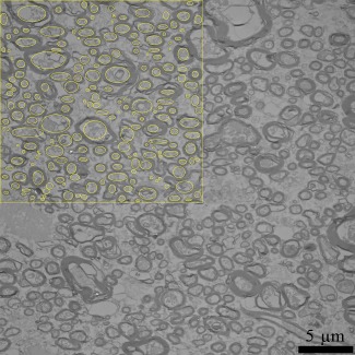
A representative electron microscopy image with the region of interest in 20 µm2 for location seven is shown. After manually adjusting the threshold parameters in ImageJ to delineate myelination, the axons were selected from five images at each location within the corpus callosum. Yellow circles are examples of axons sampled. [Color figure can be viewed at http://wileyonlinelibrary.com]
In vivo human brain study
Human data
Diffusion‐weighted and T1‐weighted images were acquired in 9 healthy human male participants (nine males aged 23–66 years) on a 7T whole body MRI research scanner (Siemens Healthcare, Erlangen, Germany) with a maximum gradient strength of 70 mT/m at a slew rate of 200 mT/m/ms. Each participant underwent a 30 minute imaging session (approximately 5 minutes for pre scans, (i) 7 minutes for structural data, (ii) 6 minutes for tractography data and (iii) 8 minutes for axon radius mapping data):
We acquired T 1‐weighted structural images for each participant at 0.75 mm3 isotropic resolution. The structural images were used as a template to depict the results of our axon radius and volume fraction mappings.
The data were acquired using a Bipolar planar diffusion imaging pulse sequence with the following parameters: TE/TR = 86/5,900 ms, Matrix = 142 by 142, iPAT = 4, bandwidth = 1,136 Hz/pixel and 50 slices with an isotropic resolution of 1.5 mm3 ensured coverage of the brain excluding the cerebellum. Gradient pulse duration = 26.82 ms and separation = 41.98 ms. Eleven b‐values between 0 and 5,000 s/mm2 in steps of 500 s/mm2 were acquired and the signal‐to‐noise ratio was maintained across all b‐values, as specified in Table 1. Images were corrected for motion and eddy current induced distortions inline on the scanner using a non‐linear registration algorithm. As an example, diffusion‐weighted images for a single slice are shown in Fig. 3.
We acquired a diffusion‐weighted data set (1.5 mm3 isotropic resolution, b‐value = 3,000 s/mm2 and 64 directions and TE/TR = 86/5,900 ms) for constrained spherical deconvolution to partition the corpus callosum into callosal regions projecting into different cortical regions. All other parameters were the same as for the other diffusion sequence.
Figure 3.
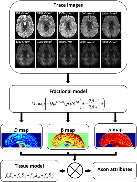
The process involved in generating axon attributes (radius and volume fraction) is outlined. Trace images computed for a representative in vivo diffusion‐weighted imaging slice with different b‐values from 500 s/mm2 to 5,000 s/mm2 in steps of 500 s/mm2 are given. The ⊗ symbol implies extraction of axon radius and volume fraction using the tissue model and parameter maps. [Color figure can be viewed at http://wileyonlinelibrary.com]
Tractography
Fibre tracking was performed using the MRtrix package in the presence of crossing fibres [Tournier et al., 2007; Tournier et al., 2004, 2012], using the streamlines algorithm [Mori and Van Zijl, 2002]. Seeds in the corpus callosum and inclusion masks of the prefrontal cortex, premotor cortex, motor cortex, parietal cortex and visual cortex were hand‐drawn [Jbabdi et al., 2013] according to Brodmann's cytotechtonic map [Duvernoy, 1999]. We chose seed regions and inclusion masks for the corpus callosum, prefrontal cortex, premotor cortex, motor cortex, parietal cortex and visual cortex. Figure 4 shows the tractography result for Participant 6 obtained using MRtrix, segmenting the corpus callosum into sections projecting to the different cortical regions. Once the corpus callosum was segmented, manual masking was performed on the corpus callosum aided by the tractography result whilst ensuring that masks were at least two image voxels inside the extent of the region in the corpus callosum identified through tractograhpy.
Figure 4.
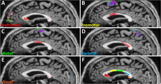
Segments of the corpus callosum projecting to various cortical regions identified using tractography. These are the actual connections used for Participant 6 projecting to (A) prefrontal (B) premotor, (C) motor, (D) parietal and (E) visual regions, and (F) shows masks identifying corpus callosum regions for which axon radius and volume fraction was calculated. [Color figure can be viewed at http://wileyonlinelibrary.com]
Axon radius and volume fraction calculation steps
Figure 3 provides a basic outline of how axon radius and volume fraction were calculated. The following outline the steps in detail:
The trace of the multiple b‐value multiple direction diffusion data was first computed for each b‐value.
A nonlinear least squares fitting algorithm (Levenberg‐Marquardt) in Matlab® [Magin et al., 2008; Zhou et al., 2010] was used to fit D, and in (2) to the trace signal across b‐values.
The tissue model was used to prototype various diffusion signal responses expected based on variations in axon radius and volume fraction of S ia (i.e., f ia).
Axon radius and volume fraction for each voxel in the corpus callosum were deduced via weighted least squares fitting of D, , and to the simulated maps.
As an example, when S0 is randomly chosen as 1,000 and for each combination of axon radius R and volume fraction fia, a simulated signal value is obtained using Eq. (8). By substituting this simulated signal value into Eq. (2) and using the method of (i), the simulated parameters of D, and can be mapped across R and fia. Axon radius and volume fraction can then be deduced through weighted least squares fitting across the three maps.
RESULTS AND DISCUSSION
Ex Vivo Corpus Callosum Findings
Ideal values for f tw (trapped water compartment contribution) in the tissue model has not been previously established. Thereby, we performed an experiment to evaluate the effect of changing f tw on the mapped axon radius and volume fraction. The value of D ∥ was calculated from the ex vivo diffusion‐weighted imaging data, and results for the seven locations are provided in Table 2. Locations along the corpus callosum shown in Fig. 1B were used in the ex vivo MRI experiment and in the electron microscopy validation. The CSF signal compartment was set to zero in the calculations and fibre direction was assumed to be into the plane of Fig. 1B.
Table 2.
D ∥ calculated from the ex vivo diffusion‐weighted imaging data at each of the seven locations along the corpus callosum (Mean ± Standard Deviation)
| Location | D∥ (µm2/ms) |
|---|---|
| 1 | 1.04 ± 0.31 |
| 2 | 0.96 ± 0.24 |
| 3 | 0.76 ± 0.18 |
| 4 | 0.88 ± 0.24 |
| 5 | 0.78 ± 0.06 |
| 6 | 0.92 ± 0.23 |
| 7 | 0.91 ± 0.26 |
Table 3.
The comparison of axon radius between the average results of nine participants with f csf = 0.05, f tw = 0.05 and D ∥=1.65 µm2/ms and histology data [Caminiti et al., 2013]
| Cortical areas | Results for nine participants | Histology result |
|---|---|---|
| Prefrontal | 1.73 ± 0.82 | 0.50 ± 0.24 |
| Premotor | 2.24 ± 0.97 | – |
| Motor | 2.22 ± 0.88 | 0.62 ± 0.37 |
| Parietal | 1.53 ± 0.85 | 0.49 ± 0.23 |
| Visual | 1.83 ± 0.72 | 0.63 ± 0.32 |
Values are in µm and are given as Mean ± Standard Deviation
It is known that the normal corpus callosum comprises thicker axons projecting into motor and visual cortical areas and thinner ones projecting into the prefrontal and parietal cortical areas [Caminiti et al., 2013; Caminiti et al., 2009; Tomasi et al., 2012] and, the mean callosal fibre density does not appear to show a significant correlation with callosal area [Aboitiz et al., 1992]. As can be seen from the histology results provided in Fig. 5A, axon radius varies along the corpus callosum as expected. We calculated the Pearson's correlation coefficient between the electron microscopy and MRI findings (see Fig. 5A) and found a volume fraction of 5% for the trapped water compartment resulted in the best axon radius result. Notably, the calculated axon radii are higher than those obtained using electron microscopy. Overestimation of axon radii can arise due to tissue shrinkage during the processing of tissue samples for electron microscopy [Bozzola and Russell, 1999; Dykstra and Reuss, 2003; Luther et al., 1988]. Accurate measures of the amount of tissue shrinkage have not been developed, which is further complicated by different tissue types exhibiting different behaviour during preparation and by the method itself used to prepare tissue. In particular, glutaraldehyde has been shown to cause 5% shrinkage in each coordinate direction for a multitude of tissues [Dykstra and Reuss, 2003], and Epon resin may cause around 12% shrinkage in the transverse axes of the axon and, as much as 40‐60% in the longitudinal axis [Höög et al., 2010; Luther et al., 1988].
Figure 5.
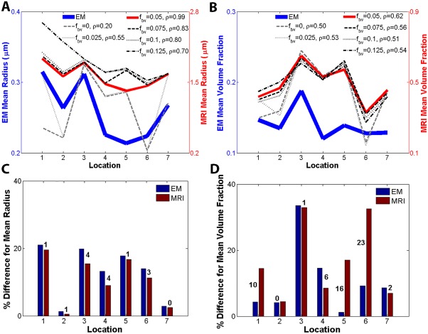
Ex vivo results comparing mean axon radius and volume fraction along the seven locations shown in Fig. 1B. (A) Mean axon radius results for 0, 0.025, 0.05, 0.075, 0.1 and 0.125 volume fractions for the trapped water compartment. This result shows that a better agreement between calculated mean radius and electron microscopy was obtained for f tw = 0.05 as confirmed by correlation coefficient ρ = 0.99. (B) Volume fraction of intra‐axonal compartment for 0, 0.025, 0.05, 0.075, 0.1 and 0.125 volume fractions for the trapped water compartment. Again the better agreement was confirmed by correlation coefficient ρ = 0.62 for f tw = 0.05. (C) Relative axon radius variation with respect to mean axon radius across the seven locations. (D) Relative volume fraction variation with respect to mean volume fraction across the seven locations. The labels on the bar graphs in (C) and (D) are the relative percent differences between calculated values from MRI data and electron microscopy. The best trend‐based results in (A) and (B) are obtained when f tw = 0.05. Notably, tissue processing associated with electron microscopy leads to tissue shrinkage making comparison of absolute values difficult, therefore a good match is implied by the trend across locations. [Color figure can be viewed at http://wileyonlinelibrary.com]
Figure 5 suggests that parameters of the anomalous diffusion equation can be used to deduce size and image voxel volume fraction occupied by the intra‐axonal space. Figure 5B shows result for intra‐axonal space volume fraction when f tw varied. Zero and 0.05 volume fractions for the trapped water fraction leads to results that mimic low‐high‐low‐high‐low trend captured using electron microscopy. In view of the axon radius results, we suggest f tw = 0.05 provides a good match between our results and electron microscopy.
Figure 5C,D provide a quantitative analysis of our findings. In Fig. 5C the axon radius at each location was assessed with respect to the mean axon radius calculated from data at all locations. The numbers show the relative difference as a percentage from the mean axon radius representative for the corpus callosum. At locations 1 to 7, the difference between our measure of axon radius and electron microscopy is 1%, 1%, 4%, 4%, 1%, 3% and 0%, giving on average 2% relative difference between the value we obtained and the validation. For the volume fraction, shown in Fig. 5D, the respective numbers across locations are 10%, 0%, 1%, 6%, 16%, 23% and 2% leading to a 8.3% difference on average.
In Vivo Corpus Callosum Findings
Based on our ex vivo findings, we decided to set f tw = 0.05 in the in vivo human brain study. We fixed D ∥ = 1.65 µm2/ms based on results of D ∥ = 1.61 µm2/ms by Rimkus et al. [2013], and Alexander et al. suggesting D ∥ = 1.7 µm2/ms [Alexander et al., 2010]. Additionally, we had to consider the partial volume of CSF within voxels. To evaluate sensitivity to changes in D ∥ and f csf, we consider the impact of 3% and 6% change in intra‐axonal space diffusivity on the calculated axon radius and volume fraction. Furthermore, we consider 100% and 200% change in f csf and how these changes impact axon radii and intra‐axonal space volume fraction results.
Figure 6A provides a box plot of the axon radius in the five corpus callosum regions evaluated across the nine participants. Correspondingly, Fig. 6B shows the intra‐axonal space volume fraction. The previously reported low‐high‐low‐high trend in axon radius [Caminiti et al., 2013] can be observed in Fig. 6A. Moreover, the mean axon radius in motor and visual areas should be larger than in the prefrontal and parietal areas [Caminiti et al., 2009, 2013]. Table III compares axon radii between the average results across the nine participants and previously published histology data reproduced from Caminiti et al. [2013]. The trend across corpus callosum regions should be compared instead of comparing absolute values, as it has been documented in detail that shrinkage occurs with histological processing [Bozzola and Russell, 1999; Dykstra and Reuss, 2003; Luther et al., 1988]. The pattern of axon radius change with region from our result is in good agreement with the histology result.
Figure 6.
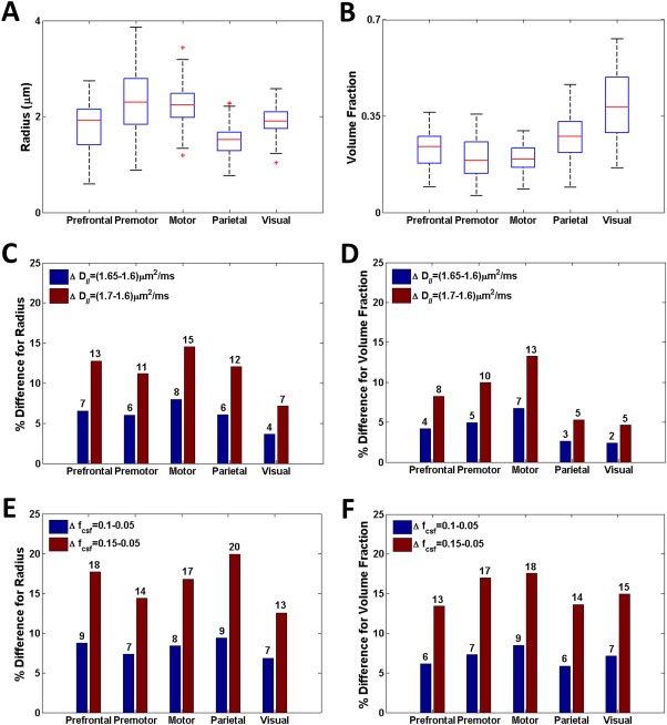
Axon radius and volume fraction results for prefrontal, premotor, motor, parietal and visual cortex callosal regions across nine healthy human participants. Values were calculated across the group: (A) radius for D ∥=1.65 µm2/ms and fcsf = 0.05, (B) volume fraction for D ∥=1.65 µm2/ms and fcsf = 0.05, (C) Sensitivity of radii to changes in axon diffusivity for fcsf = 0.05, (D) volume fraction sensitivity to changes in axon diffusivity fcsf = 0.05, (E) radii sensitivity to changes in CSF volume fraction for D ∥=1.65 µm2/ms, and (F) volume fraction sensitivity to changes in CSF volume fraction for D ∥=1.65 µm2/ms. The labels on the bar graphs in (C) to (F) are the percent differences for each of the cases considered. [Color figure can be viewed at http://wileyonlinelibrary.com]
Aboitiz et al. [1992] did not find a significant correlation between mean callosal fiber density and callosal area, and other results for intra‐axonal space volume fraction are not available. From Fig. 6B, it can be seen that intra‐axonal space volume fraction generally increases in the visual region of the corpus callosum in comparison to other callosal areas, and premotor and motor areas have the smallest volume fractions. Table 4 summarises results obtained from nine participants.
Table 4.
The comparison of volume fraction between the average results of nine human participants with f csf = 0.05, f tw = 0.05 and D ∥ = 1.65 µm2/ms
| Cortical areas | Results for nine participants |
|---|---|
| Prefrontal | 0.23 ± 0.08 |
| Premotor | 0.20 ± 0.09 |
| Motor | 0.19 ± 0.07 |
| Parietal | 0.29 ± 0.15 |
| Visual | 0.39 ± 0.18 |
Figure 6C,D provide axon radius and intra‐axonal space volume fraction sensitivity results when D ∥ is changed by 3% and 6% and f csf = 0.05. Since the change in axon radius approximately doubles when changing D ∥ from 0.05 µm2/ms to 0.10 µm2/ms, we expect a linear effect on axon radius due to change in diffusivity about D ∥ = 1.65 µm2/ms. A 1% change in diffusivity impacts our calculated value for axon radius by 2% in the prefrontal, premotor and parietal regions. In the motor regions the change increases to around 3% and in the visual area it decreases to around 1%. In Fig. 6D, the effect on volume fraction due to a change in D∥ is also linear about D ∥= 1.65 µm2/ms. The impact of changing D ∥ has a slightly smaller percentage impact on volume fraction, and across the regions the trend appears to be the same as the one in Fig. 6C.
Figure 6E,F provide axon radius and intra‐axonal space volume fraction sensitivity results when f csf is changed by 100% and 200% and D ∥=1.65 µm2/ms. The effect on axon radius and volume fraction due to a change in f csf only is approximately linear about f csf = 0.05. However, a 10% change in f csf leads to around 1% change in axon radius and less than 1% in volume fraction. From these results we may conclude that our measure of axon radius and volume fraction is as much as 20 times more sensitive to changes in D ∥ than f csf.
The results presented here rely on a tissue model to relate parameters of the anomalous diffusion equation to axon radius and volume fraction. We used the tissue model proposed by Alexander et al., which comprises of four tissue compartments [Alexander et al., 2010]. The model is a simplification of tissue structure and composition, as only axonal structures are considered. Furthermore, a single axon radius is assumed in the tissue model and effects due to axon distribution are not considered. The collected diffusion‐weighted images may be influenced by the distribution of axon radius within the corpus callosum. The model also assumes a single axon orientation within the voxel; this is unlikely to have an impact on our findings because axons are generally aligned in the corpus callosum. It is also assumed that changes due to water exchange between compartments is negligible compared to changes due to water bound to membranes and other subcellular structures or trapped within small tissue compartments. Using the ex vivo data, we empirically tested the effect of the trapped water compartment on the axon radius result. We found that a 5% volume fraction for the trapped water compartment resulted in the best fit (see Fig. 5A). A better understanding of the contribution from the trapped water compartment could potentially be obtained from future in‐depth histological and histochemical analyses of resected brain tissue.
The axon radius influences only the restricted signal compartment and the analytic form of this compartment was derived based on the narrow pulse approximation [Vangelderen et al., 1994], that is, gradient pulse duration should be much shorter than diffusion time. In the ex vivo and in vivo experiments the ratio of gradient pulse duration to gradient pulse separation (i.e., diffusion time) was 0.64. It is, however, not clear how this assumption influences the calculated axon radius and volume fraction. It is plausible that additional sensitivity to measuring axon radius and volume fraction can be gained by optimally setting values for gradient pulse duration and separation. However, values for gradient pulse separation and duration can only be set within practical limits for scanners. It is plausible that additional sensitivity and accuracy can be gained by carefully selecting values for these parameters and the ratio between them. Diffusion signal attenuates and signal‐to‐noise ratio decreases with an increase in echo time. Hence, echo time places a practical limit on the value set for diffusion time. Appropriate selection of gradient pulse separation and duration would involve an in‐depth analysis of how model parameters (D, and ) are influenced by changes in these parameters, which is beyond the scope of the work presented here.
Diffusion can be considered to be anomalous in space or time or both. Here we considered the case of the space fractional Bloch‐Torrey equation. Burcaw et al. found a contradiction between histology‐based evidence and anomalous or fractal diffusion models in the mouse brain [Burcaw et al., 2015]. Their findings were based on anomalous or fractal diffusion in time, and not in space, as was the case for our work. Our findings suggest that space fractional anomalous diffusion models have a place in mapping changes in brain microstructure, as has been noted in a previous study [Meerschaert et al., 2016]. Thereby, in the case of neurological diseases and disorders wherein spatial reorganisation of tissue microstructure is present, the parameters of the space fractional anomalous diffusion model may provide additional insight which may help with diagnosis and prognosis.
CONCLUSIONS
We mapped axon radius and volume fraction in the corpus callosum of the ex vivo and in vivo human brain, and validated ex vivo findings using electron microscopy. We found a good agreement between ex vivo and electron microscopy results, and in vivo findings showed the previously reported trend across the corpus callosum. The framework proposed by Alexander et al., adopted in our work, is based on intra‐ and extra‐axonal diffusion (i.e., the approach named CHARMED) [Alexander et al., 2010]. This tissue model may not generally be applicable across white matter regions, particularly those regions where tissue compartments are able to undergo water exchange. Future work should consider tissue models that can account for different amount of water exchange between compartments, which may lead to further decreases in the relative differences found between our ex vivo MRI results and electron microscopy validation.
Our approach of using anomalous diffusion model developed using fractional calculus demonstrates the importance of choosing appropriate models for challenges faced in neuroscience. The ability to map the microstructural properties of tissues can no doubt provide insight into neurodegenerative diseases and disorders, and help with the development of biomarkers for the purpose of disease detection and monitoring of tissue changes over time. This work may potentially lead to further studies that focus on certain white matter diseases and disorders, and to studies in which connectivity afforded by white matter pathways plays an important role.
ACKNOWLEDGMENTS
The authors acknowledge the help by Aiman Al Najjar from Centre for Advanced Imaging of the University of Queensland, and Thorsten Feiweier and Siemens Healthcare for provision of the prototype sequence for the in vivo diffusion weighted imaging. The authors also acknowledge the facilities, and the scientific and technical assistance, of the Australian Microscopy & Microanalysis Research Facility at the Centre for Microscopy and Microanalysis at the University of Queensland. The authors acknowledge the help by Richard Webb and Robyn Webb from Centre for Microscopy and Microanalysis of the University of Queensland. Dr Qiang Yu acknowledges the University of Queensland for awarding a UQ Postdoctoral Research Fellowship for financial support.
REFERENCES
- Aboitiz F, Scheibel AB, Fisher RS, Zaidel E (1992): Fiber composition of the human corpus callosum. Brain Res 598:143–153. [DOI] [PubMed] [Google Scholar]
- Abragam A (2002): Principles of nuclear magnetism. Oxford: Oxford University Press. [Google Scholar]
- Alexander DC (2008): A general framework for experiment design in diffusion MRI and its application in measuring direct tissue‐microstructure features. Magn Reson Med 60:439–448. [DOI] [PubMed] [Google Scholar]
- Alexander DC, Hubbard PL, Hall MG, Moore EA, Ptito M, Parker GJM, Dyrby TB (2010): Orientationally invariant indices of axon diameter and density from diffusion MRI. NeuroImage 52:1374–1389. [DOI] [PubMed] [Google Scholar]
- Assaf Y, Freidlin RZ, Rohde GK, Basser PJ (2004): New modeling and experimental framework to characterize hindered and restricted water diffusion in brain white matter. Magn Reson Med 52:965–978. [DOI] [PubMed] [Google Scholar]
- Assaf Y, Blumenfeld‐Katzir T, Yovel Y, Basser PJ (2008): AxCaliber: A method for measuring axon diameter distribution from diffusion MRI. Magn Reson Med 59:1347–1354. [DOI] [PMC free article] [PubMed] [Google Scholar]
- Barazany D, Basser PJ, Assaf Y (2009): In‐vivo measurement of the axon diameter distribution in the corpus callosum of a rat brain. Brain 132:1210–1220. [DOI] [PMC free article] [PubMed] [Google Scholar]
- Basser PJ, Matiello J, LeBihan D (1994): MR diffusion tensor spectroscopy and Imaging. Biophys J 66:259–267. [DOI] [PMC free article] [PubMed] [Google Scholar]
- Bouchaud JP, Georges A (1990): Anomalous diffusion in disordered media: Statistical mechanisms, models and physical applications. Phys Rep 195:127–293. [Google Scholar]
- Bozzola JJ, Russell LD. (1999): Electron Microscopy, Principles and Techniques for Biologists. Sudbury: Jones and Bartlett. [Google Scholar]
- Braitenberg V, Schüz A. (1998): Cortex: Statistics and Geometry of Neuronal Connectivity. Berlin: Springer. [Google Scholar]
- Burcaw LM, Fieremans E, Novikov DS (2015): Mesoscopic structure of neuronal tracts from time‐dependent diffusion. NeuroImage 114:18–37. [DOI] [PMC free article] [PubMed] [Google Scholar]
- Caminiti R, Ghaziri H, Galuske R, Hof PR, Innocenti GM (2009): Evolution amplified processing with temporally dispersed slow neuronal connectivity in primates. Proc Natl Acad Sci 106:19551–19556. [DOI] [PMC free article] [PubMed] [Google Scholar]
- Caminiti R, Carducci F, Piervincenzi C, Battaglia‐Mayer A, Confalone G, Visco‐Comandini F, Pantano P, Innocenti GM (2013): Diameter, length, speed, and conduction delay of callosal axons in macaque monkeys and humans: Comparing data from histology and magnetic resonance imaging diffusion tractography. J Neurosci 33:14501–14511. [DOI] [PMC free article] [PubMed] [Google Scholar]
- Cluskey S, Ramsden DB (2001): Mechanisms of neurodegeneration in amyotrophic lateral sclerosis. Mol Pathol 54:386–392. [PMC free article] [PubMed] [Google Scholar]
- Donskaya IS (1973): Bloch equations with diffusion terms for rotational motion in fluids. Sov Phys J 16:29–32. [Google Scholar]
- Duvernoy HM. (1999): The Human Brain: Surface, Three‐Dimensional Sectional Anatomy With MRI, and Blood Supply. New York: Springer‐Wien. [Google Scholar]
- Dykstra MJ, Reuss LE. (2003): Biological Electron Microscopy: Theory, Techniques, and Troubleshooting. New York: Springer. [Google Scholar]
- Dyrby TB, Søgaard LV, Hall MG, Ptito M, Alexander DC (2013): Contrast and stability of the axon diameter index from microstructure imaging with diffusion MRI. Magn Reson Med 70:711–721. [DOI] [PMC free article] [PubMed] [Google Scholar]
- Gao Q, Srinivasan G, Magin R, Zhou X (2011): Anomalous diffusion measured by a twice‐refocused spin echo pulse sequence: analysis using fractional order calculus. J Magn Reson Imaging 33:1177–1183. [DOI] [PMC free article] [PubMed] [Google Scholar]
- Gorenflo R, Mainardi F, Moretti D, Paradisi P (2002): Time fractional diffusion: a discrete random walk approach. Nonlinear Dyn 29:129–143. [Google Scholar]
- Hall M, Barrick T (2008): From diffusion‐weighted MRI to anomalous diffusion imaging. Magn Reson Med 59:447–455. [DOI] [PubMed] [Google Scholar]
- Heads T, Pollock M, Robertson A, Sutherland WH, Allpress S (1991): Sensory nerve pathology in amyotrophic lateral sclerosis. Acta Neuropathol 82:316–320. [DOI] [PubMed] [Google Scholar]
- Hilfer R. 2000. Applications of Fractional Calculus in Physics. New York: World Scientific Publishing. [Google Scholar]
- Höög JL, Gluenz E, Vaughan S, Gull K (2010): Ultrastructural investigation methods for Trypanosoma brucei. Methods Cell Biol 96:175–196. [DOI] [PubMed] [Google Scholar]
- Hughes BD (1995): Random Walks and Random Environments, Vol. 1: random walks. Oxford: Oxford University Press. [Google Scholar]
- Hughes JR (2007): Autism: the first firm finding= underconnectivity? Epilepsy Behav 11:20–24. [DOI] [PubMed] [Google Scholar]
- Hursh JB (1939): The properties of growing nerve fibers. Am J Physiol 127:140–153. [Google Scholar]
- Ingo C, Sui Y, Chen Y, Parrish TB, Webb AG, Ronen I (2015): Parsimonious continuous time random walk models and kurtosis for diffusion in magnetic resonance of biological tissue. Front Phys 3:11. [DOI] [PMC free article] [PubMed] [Google Scholar]
- Jbabdi S, Lehman JF, Haber SN, Behrens TE (2013): Human and monkey ventral prefrontal fibers use the same organizational principles to reach their targets: tracing versus tractography. J Neurosci 33:3190–3201. [DOI] [PMC free article] [PubMed] [Google Scholar]
- Kaplan JI (1959): Application of the diffusion‐modified bloch equation to electron spin resonance in ordinary and ferromagnetic metals. Phys Rev 115:575–577. [Google Scholar]
- Khanafer K, Vafai K, Kangarlu A (2003): Water diffusion in biomedical systems as related to magnetic resonance imaging. Magn Reson Imaging 21:17–31. [DOI] [PubMed] [Google Scholar]
- Kilbas AA, Srivastava HM, Trujillo JJ (2006): Theory and Applications of Fractional Differential Equations. Amsterdam: Elsevier. [Google Scholar]
- Kimmich R (2002): Strange kinetics, porous media, and NMR. Chem Phys 284:253–285. [Google Scholar]
- Klafter J, Shlesinger MF, Zumofen G (1996): Beyond brownian motion. Phys Today 49:33–39. [Google Scholar]
- Köpf M, Metzler R, Haferkamp O, Nonnenmacher TF (1998): NMR studies of anomalous diffusion in biological tissues: experimental observation of Lévy stable processes In: Fractals in Biology and Medicine. Birkhäuser Basel: Springer. pp 354–364. [Google Scholar]
- Liang Y, Ye AQ, Chen W, Gatto RG, Colon‐Perez L, Mareci TH, Magin RL (2016): A fractal derivative model for the characterization of anomalous diffusion in magnetic resonance imaging. Commun Nonlinear Sci Numer Simulat 39:529–537. [Google Scholar]
- Luther PK, Lawrence MC, Crowther RA (1988): A method for monitoring the collapse of plastic sections as a function of electron dose. Ultramicroscopy 24:7–18. [DOI] [PubMed] [Google Scholar]
- Magin R, Abdullah O, Baleanu D, Zhou X (2008): Anomalous diffusion expressed through fractional order differential operators in the Bloch‐Torrey equation. J Magn Reson 190:255–270. [DOI] [PubMed] [Google Scholar]
- Magin R, Feng X, Baleanu D (2009): Fractional calculus in NMR. Magn Reson Engr 34:16–23. [Google Scholar]
- Magin RL, Li W, Velasco MP, Trujillo J, Reiter DA, Morgenstern A, Spencer RG (2011): Anomalous NMR relaxation in cartilage matrix components and native cartilage: Fractional‐order models. J Magn Reson 210:184–191. [DOI] [PMC free article] [PubMed] [Google Scholar]
- Magin RL, Ingo C, Colon‐Perez L, Triplett W, Mareci TH (2013): Characterization of anomalous diffusion in porous biological tissues using fractional order derivatives and entropy. Microporous Mesoporous Mater 178:39–43. [DOI] [PMC free article] [PubMed] [Google Scholar]
- Meerschaert MM, Magin RL, Allen QY (2016): Anisotropic fractional diffusion tensor imaging. J Vib Control 22:2211–2221. [DOI] [PMC free article] [PubMed] [Google Scholar]
- Metzler R, Klafter J (2000): The random walk's guide to anomalous diffusion: a fractional dynamics approach. Phys Rep 339:1–77. [Google Scholar]
- Metzler R, Klafter J (2004): The restaurant at the end of the random walk: recent developments in the description of anomalous transport by fractional dynamics. J Phys A 37:R161–R208. [Google Scholar]
- Mori S, Van Zijl PCM (2002): Fiber tracking: Principles and strategies‐a technical review. NMR Biomed 15:468–480. [DOI] [PubMed] [Google Scholar]
- Mori S, Zhang J (2006): Principles of diffusion tensor imaging and its applications to basic neuroscience research. Neuron 51:527–539. [DOI] [PubMed] [Google Scholar]
- Njiokiktjien C, de Sonneville L, Vaal L (1994): Callosal size in children with learning disabilities. Behav Brain Res 64:213–218. [DOI] [PubMed] [Google Scholar]
- Norris D (2001): The effects of microscopic tissue parameters on the diffusion weighted magnetic resonance imaging experiment. NMR Biomed 14:77–93. [DOI] [PubMed] [Google Scholar]
- Ong HH, Wright AC, Wehrli SL, Souza A, Schwartz ED, Hwang SN, Wehrli FW (2008): Indirect measurement of regional axon diameter in excised mouse spinal cord with q‐space imaging: Simulation and experimental studies. NeuroImage 40:1619–1632. [DOI] [PMC free article] [PubMed] [Google Scholar]
- Panagiotaki E, Schneider T, Siow B, Hall MG, Lythgoe MF, Alexander DC (2012): Compartment models of the diffusion MRI signal in brain white matter: A taxonomy and comparison. NeuroImage 59:2241–2254. [DOI] [PubMed] [Google Scholar]
- Piven J, Bailey J, Ranson BJ, Arndt S (1997): An MRI study of the corpus callosum in autism. Am J Psychiatry 154:1051–1056. [DOI] [PubMed] [Google Scholar]
- Price WS. 2009. NMR Studies of Translational Motion: Principles and Applications. New York: Cambridge University Press. [Google Scholar]
- Randall PL (1983): Schizophrenia, abnormal connection, and brain evolution. Med Hypotheses 10:247–280. [DOI] [PubMed] [Google Scholar]
- Rice D, Barone S Jr (2000): Critical periods of vulnerability for the developing nervous system: evidence from humans and animal models. Environ Health Perspect 108:511–533. [DOI] [PMC free article] [PubMed] [Google Scholar]
- Rimkus CD, Junqueira TD, Callegaro D, Otaduy MC, Leite CD (2013): Segmented corpus callosum diffusivity correlates with the expanded disability status scale score in the early stages of relapsing‐remitting multiple sclerosis. Clinics 68:1115–1120. [DOI] [PMC free article] [PubMed] [Google Scholar]
- Ringo JL, Doty RW, Demeter S, Simard PY (1994): Time is of the essence: a conjecture that hemispheric specialization arises from interhemispheric conduction delay. Cereb Cortex 4:331–343. [DOI] [PubMed] [Google Scholar]
- Ritchie JM (1982): On the relation between fibre diameter and conduction velocity in myelinated nerve fibres. Proc R Soc B 217:29–35. [DOI] [PubMed] [Google Scholar]
- Rohmer D, Gullberg GT (2006): A Bloch‐Torrey equation for diffusion in a deforming media. Tech. Rep., University of California, Technical Report Paper LBNL‐61295. [Google Scholar]
- Sen PN (2003): Time‐dependent diffusion coefficient as a probe of the permeability of the pore wall. J Chem Phys 119:9871–9876. [Google Scholar]
- Shlesinger MF, Zaslavsky GM, Klafter J (1993): Strange kinetics. Nature 363:31–37. [Google Scholar]
- Speck O, Ernst T, Chang L (2001): Biexponential modeling of multigradient‐echo MRI data of the brain. Magn Reson Med 45:1116–1121. [DOI] [PubMed] [Google Scholar]
- Stapf S, Kimmich R, Seitter RO (1995): Proton and deuteron field‐cycling NMR relaxometry of liquids in porous glasses: Evidence for Lévy‐walk statistics. Phys Rev Lett 75:2855–2858. [DOI] [PubMed] [Google Scholar]
- Stapf S (2002): NMR investigations of correlations between longitudinal and transverse displacements in flow through random structured media. Chem Phys 284:369–388. [Google Scholar]
- Szafer A, Zhong J, Gore JC (1995): Theoretical model for water diffusion in tissues. Magn Reson Med 33:697–712. [DOI] [PubMed] [Google Scholar]
- Tomasi S, Caminiti R, Innocenti GM (2012): Areal differences in diameter and length of corticofugal projections. Cereb Cortex 22:1463–1472. [DOI] [PubMed] [Google Scholar]
- Torrey HC (1956): Bloch equations with diffusion terms. Phys Rev 104:563–565. [Google Scholar]
- Tournier JD, Calamante F, Gadian DG, Connelly A (2004): Direct estimation of the fiber orientation density function from diffusion‐weighted MRI data using spherical deconvolution. Neuroimage 23:1176–1185. [DOI] [PubMed] [Google Scholar]
- Tournier JD, Calamante F, Connelly A (2007): Robust determination of the fibre orientation distribution in diffusion MRI: non‐negativity constrained super‐resolved spherical deconvolution. Neuroimage 35:1459–1472. [DOI] [PubMed] [Google Scholar]
- Tournier JD, Calamante F, Connelly A (2012): MRtrix: diffusion tractography in crossing fibre regions. Int J Imag Syst Tech 22:53–66. [Google Scholar]
- Upadhyaya A, Rieu JP, Glazier JA, Sawada Y (2001): Anomalous diffusion and non‐Gaussian velocity distribution of Hydra cells in cellular aggregates. Phys A 293:549–558. [Google Scholar]
- van Gelderen P, Despres D, Vanzijl PCM, Moonen CTW (1994): Evaluation of restricted diffusion in cylinders. Phosphocreatine in rabbit leg muscle. J Magn Reson Ser B 103:255–260. [DOI] [PubMed] [Google Scholar]
- Waxman SG (1980): Determinants of conduction velocity in myelinated nerve fibers. Muscle Nerve 3:141–150. [DOI] [PubMed] [Google Scholar]
- Yablonskiy DA, Sukstanskii AL (2010): Theoretical models of the diffusion weighted MR signal. NMR Biomed 23:661–681. [DOI] [PMC free article] [PubMed] [Google Scholar]
- Yu Q, Liu F, Anh V, Turner I (2008): Solving linear and nonlinear space‐time fractional reaction‐diffusion equations by Adomian decomposition method. Int J Numeric Methods Eng 74:138–158. [Google Scholar]
- Yu Q, Liu F, Turner I, Burrage K (2012): A computationally effective alternating direction method for the space and time fractional Bloch‐Torrey equation in 3‐D. Appl Math Comput 219:4082–4095. [Google Scholar]
- Yu Q, Liu F, Turner I, Burrage K (2013a): Numerical investigation of three types of space and time fractional Bloch‐Torrey equations in 2D. Cent Eur J Phys 11:646–665. [DOI] [PubMed] [Google Scholar]
- Yu Q, Liu F, Turner I, Burrage K (2013b): Stability and convergence of an implicit numerical method for the space and time fractional Bloch‐Torrey equation. Phil Trans R Soc A 371:20120150 Available at: 10.1098/rsta.2012.0150 [DOI] [PubMed] [Google Scholar]
- Zaslavsky G (2002): Chaos, fractional kinetics, and anomalous transport. Phys Rep 371:461–580. [Google Scholar]
- Zhang H, Hubbard PL, Parker GJM, Alexander DC (2011): Axon diameter mapping in the presence of orientation dispersion with diffusion MRI. NeuroImage 56:1301–1315. [DOI] [PubMed] [Google Scholar]
- Zhou X, Gao Q, Abdullah O, Magin R (2010): Studies of anomalous diffusion in the human brain using fractional order calculus. Magn Reson Med 63:562–569. [DOI] [PubMed] [Google Scholar]