Age prediction on the basis of brain anatomical measures

Abstract

In this study, we examined whether age can be predicted on the basis of different anatomical features obtained from a large sample of healthy subjects (n = 3,144). From this sample we obtained different anatomical feature sets: (1) 11 larger brain regions (including cortical volume, thickness, area, subcortical volume, cerebellar volume, etc.), (2) 148 cortical compartmental thickness measures, (3) 148 cortical compartmental area measures, (4) 148 cortical compartmental volume measures, and (5) a combination of the above‐mentioned measures. With these anatomical feature sets, we predicted age using 6 statistical techniques (multiple linear regression, ridge regression, neural network, k‐nearest neighbourhood, support vector machine, and random forest). We obtained very good age prediction accuracies, with the highest accuracy being R ² = 0.84 (prediction on the basis of a neural network and support vector machine approaches for the entire data set) and the lowest being R ² = 0.40 (prediction on the basis of a k‐nearest neighborhood for cortical surface measures). Interestingly, the easy‐to‐calculate multiple linear regression approach with the 11 large brain compartments resulted in a very good prediction accuracy (R ² = 0.73), whereas the application of the neural network approach for this data set revealed very good age prediction accuracy (R ² = 0.83). Taken together, these results demonstrate that age can be predicted well on the basis of anatomical measures. The neural network approach turned out to be the approach with the best results. In addition, it was evident that good prediction accuracies can be achieved using a small but nevertheless age‐representative dataset of brain features. Hum Brain Mapp 38:997–1008, 2017. © 2016 Wiley Periodicals, Inc.

Abbreviations

CC

Corpus callosum

ICV

Intracranial volume

KNN

K‐nearest neighbor

LDA

Linear discriminant analysis

MLR

Multiple linear regression

NN

Neural network

ROI

Region of interest

RR

Ridge regression

RVM

Relevance vector machine

SVM

Support vector machine

VBM

Voxel‐based morphometry

INTRODUCTION

It is a well‐known fact that the brain changes during aging. An often‐reported finding is that particular brain areas change more than others [Fjell and Walhovd, 2010; Fjell et al., 2009b]. However, this issue is far from clear since reported age‐related brain changes and differences differ across studies and methods used. Combining anatomical data from six different samples, Fjell and colleagues [Fjell et al., 2009b] revealed that the frontal cortex (especially the superior, middle, and inferior frontal gyri), and some parts of the temporal (e.g., the middle temporal gyri) and parietal cortex (e.g., the precuneus, the inferior and superior parietal cortices, and the temporo‐parietal junction) are subject to age‐related cortical thinning. The strongest effects were seen in the superior and inferior frontal gyri, as well as in the superior parts of the temporal lobe. In contrast, the inferior temporal lobe and anterior cingulate cortices were relatively less affected by age [Fjell et al., 2009b].

Most studies examining age‐effects on brain tissue, however, have focused on cortical measures, with only a few studies focusing on possible age‐related differences with respect to subcortical volumes (e.g., thalamus, caudate, amygdala, hippocampus, putamen, pallidum, and accumbens) [Fjell and Walhovd, 2010; Jäncke et al., 2015; Li et al., 2014; Tang et al., 2013]. Similar to studies investigating cortical regions, these studies have demonstrated substantial subcortical volume losses during the course of healthy aging.

Although studies using between‐group statistics may indicate the typical age‐related anatomical differences, it has been argued that between‐group analyses might be less useful for automatic diagnosis of group differences and age‐related diseases [Seidman et al., 2004]. The wide utilization of modern machine learning techniques in the neuroimaging community has made it possible for researchers to discover biomarkers of aging and to develop automatic classification systems. In addition, it may prove helpful to delineate a typical pattern of anatomical measures for a particular age in order to more precisely identify deviations from normal aging.

In this context, many efforts have been made to use structural and functional magnetic resonance imaging (sMRI and fMRI, respectively) to classify different patient groups and to statistically separate them from healthy control subjects. For example, several studies have tried to classify Alzheimer's and schizophrenia patients using anatomical measures [Fan et al., 2008; Hinrichs et al., 2009; Hinrichs et al., 2011]. In addition, several attempts have been made to predict age on the basis of anatomical data. The underlying idea of these studies is to detect possible discrepancies between predicted and chronological age, which might help identifying pathological structural changes. Only a handful of studies have been published so far conducting age estimation based on MRI scans. Lao et al. [2004] used support vector machine (SVM) techniques to classify elderly subjects into one of four age groups on the basis of anatomical measures and reached an accuracy rate of 90%. Ashburner [2007] applied an algorithm for “diffeomorphic” image registration to estimate the age of healthy subjects and reported good age prediction accuracy. Neeb and colleagues [Neeb et al., 2006] used brain water maps (which is a new method for the absolute and quantitative mapping of water content in vivo) to predict age and gender in 44 healthy volunteers aged 23–74 years. They applied a linear discriminant analysis (LDA) with jackknife cross‐validation for age prediction and obtained good classification performance. Age predictions have also been conducted in the so‐called BrainAge project from the Jena group [Franke et al., 2015; Franke et al., 2012; Franke et al., 2014; Franke et al., 2010; Gaser et al., 2013]. These studies predicted age in the context of voxel‐based morphometry (VBM) methods using a relevance vector machine (RVM) technique. Using this technique, they obtained a correlation between predicted and true age of r = 0.92.

Several classification techniques have been used so far, ranging from “classical” LDA [Kasparek et al., 2011; Leonard et al., 1999; Nakamura et al., 2004; Takayanagi et al., 2011], and linear and non‐linear regression analysis to various variants of SVM approaches [Ashburner, 2007; Castro et al., 2014; Dai et al., 2012; Fan et al., 2008; Hinrichs et al., 2011; Klöppel et al., 2012; Sato et al., 2012; Schnack et al., 2014; Wachinger et al., 2015; Wachinger et al., 2014]. Which of these techniques are best suited for age prediction is an open question that needs further investigation.

All studies that have predicted age on the basis of anatomical data have worked with cross‐sectional datasets. Thus, cohort effects could possibly have influenced the morphological features. For example, nutritional status, education, health, and social interactions have substantially changed within the last 40–60 years. Since there is ample evidence available demonstrating that these factors influence brain anatomy and body size [de Bruin et al., 2005; Pannacciulli et al., 2006; Taki et al., 2004; Taki et al., 2006], it is necessary to control for brain/head size. Here we used intracranial volume (ICV). ICV more closely indicates head size rather than brain size, since it comprises brain tissue, meninges, cerebrospinal fluid, and interstitial volumes. ICV does not correlate perfectly with forebrain volume (R ² = 0.58) [Jäncke et al., 2015], demonstrating that more than 40 percent of ICV variance is unrelated to brain tissue. In addition, it has been shown that small brains in terms of ICV exploit the space within the skull more efficiently than larger brains [Jäncke et al., 2015]. Conversely, there is disproportionately more space available for brain tissue in larger brains. To account for these non‐brain‐tissue influences, it would be necessary to control for ICV influences when predicting age on the basis of anatomical measures.

A major problem with attempts to predict age from anatomical measures is the problem of over‐fitting, which is present even when using relatively small sample sizes. In this study, we will use brain anatomical measures from a large sample in freely available databases, in addition to samples from our own laboratory. This amounts to a sample of 3,144 subjects spanning an age range from 8 to 96 years. Secondly, in contrast with the aforementioned studies, we will use cortical thickness, volume and area measures from 148 regions of interest obtained using the FreeSurfer analysis tool. In addition, we will use subcortical volume measures and anatomical measures of larger brain regions (mean cortical thickness, volume, and area, as well as mean subcortical volume) in order to examine whether these larger ROIs will provide similar or even better classification results than the collection of small ROIs. Using this collection of anatomical measures, we will explicitly answer the following questions: (1) Is it possible to predict age on the basis of a combination of anatomical measures? (2) Which combination of anatomical measures is most important in predicting age? (3) Do different classification techniques (linear discriminant analysis, SVMs, ridge regression, random forest, or neural network classification) substantially differ in terms of their classification accuracy?

METHODS

Subjects/Database

The sample used for this study comprises three samples (Table 1): 1) the Zurich sample from our research group [partly taken from Jäncke et al., 2015], 2) the publicly available samples from the 1000 Functional Connectomes Project (http://fcon_1000.projects.nitrc.org), and 3) some other freely available samples (see Table 1). Only subjects who reported no history of neurological diseases (e.g., Parkinson's disease, Alzheimer's disease), mental disorders (e.g., depression), diseases of the haematopoietic system (e.g., anemia, leukemia), or traumatic brain injuries were included, and those suffering from migraines, diabetes or tinnitus were excluded from participation. The whole sample contained 4,167 subjects from which we excluded 1023 subjects according to the following explicit reasons: (1) 304 subjects were excluded because they suffered from neurological or psychiatric disorders, (2) 422 subjects were excluded because there was no information available about gender and age, and (3) 297 subjects were excluded because the anatomical data were too noisy for the FreeSurfer analysis. We performed our calculations on the remaining 3,144 subjects. The ages of this sample ranged from 7 to 96 years (male: 8–93 years, mean = 32.69 years, s.d. = 19.4 years; female: 7–96 years, mean = 35.7 years, s.d. = 20.7 years).

Table 1.

Description of the samples and studies from which the anatomical data were obtained

Database/study number	# Male	# Female	Mean (age‐man)	Mean (age‐woman)	SD (age man)	SD (age woman)	Reference
ABIDE	99	18	13.21	11.23	2.58	2.33	FCN 1000
ADHD 200	138	132	11.33	10.84	2.00	2.20	FCN 1000
AnnArbor	34	20	31.99	40.24	21.34	25.82	FCN 1000
Atlanta	13	15	32	29.93	10.78	9.33	FCN 1000
Baltimore	8	15	30.38	28.67	4.98	5.78	FCN 1000
Beijing	76	122	21.44	21.17	1.83	1.83	FCN 1000
Cambridge	75	123	20.99	21.05	2.14	2.41	FCN 1000
Cleveland	11	20	43.18	43.75	10.31	11.79	FCN 1000
ICBM	40	45	44.38	43.76	15.44	20.13	FCN 1000
IXI	250	313	46.09	50.2	16.45	16.4	FCN 1000
Milwaukee	15	31	51.93	54.38	4.89	6.1	FCN 1000
New York	49	53	26.09	25.33	10.74	9.23	FCN 1000
OASIS	159	256	49.5	54.6	25.03	24.92	Marcus et al., 2007
Oulu	37	64	21.41	21.59	0.6	0.56	FCN 1000
Study 01	34	45	23.58	22.91	3.61	2.41	Mondadori et al., 2007
Study 02	3	12	24.67	28.75	2.08	2.93	unpublished
Study 03	18	32	51.27	50.15	7.78	7.68	Bezzola et al., 2011
Study 04	16	24	35.04	35	12.71	12.61	Dall'Acqua et al., 2016
Study 05	292	337	42.89	42.1	21.99	21.7	Jäncke et al., 2015a
Study 06	7	2	34.12	25.18	10.68	5.66	Langer et al., 2012
Study 07	27	7	35.33	33.85	8.74	7.24	unpublished
Study 08	13	16	29.23	24.75	5.48	4.15	Klein et al., 2015
Study 09	0	15		31.1		8.47	unpublished
Study 10	13	0	49.31		14.49		Hilti et al., 2013

Abbreviations: ABIDE: Autism Brain Imaging Data Exchange (http://fcon_1000.projects.nitrc.org/indi/abide/); ADHD: Attention Deficit Hyperactivity Disorder; FCN 1000: 1000 Functional Connectomes Project (https://www.nitrc.org/projects/fcon_1000/); ICBM: International Consortium for Brain Mapping; IXI: Information eXtraction from Images ( http://brain-development.org/ixi-dataset /); OASIS: Open Access Series of Imaging Studies (http://www.oasis-brains.org/); # number of subjects.

Preprocessing of Anatomical Data

For this paper we estimated compartmental cortical volumes, thickness, and surface area measures for 148 brain regions using the FreeSurfer anatomical region of interest (ROI) tool [Destrieux et al., 2010; Fischl et al., 2004a; Fischl et al., 2004b]. Here we used FreeSurfer version 5.3. The ROIs comprise brain regions from the left and right cortices. In addition, we calculated subcortical (thalamus, putamen, pallidum, caudatus, hippocampus, amygdala, and accumbens) and total subcortical volume, the volumes of the corpus callosum (CC), cerebrospinal fluid, total white matter hypo‐intensity, and the brainstem volume (midbrain, pons, medulla oblongata and superior cerebellar peduncle), total brain volume, and mean global cortical thickness and total surface area. The subcortical anatomical measures were obtained using the FreeSurfer's subcortical segmentation tool. A special note is warranted for the CC, which is also included in our data set. In FreeSurfer, the CC is not only segmented into a midsagittal slice but continues laterally into both hemispheres producing a multi‐slice three‐dimensional slab. Thus, FreeSurfer provides a three‐dimensional segmentation of the CC, which is different to many studies using CC measures to study structure‐function relationships.

In order to normalize all anatomical measures to brain/head size and to reduce variance we computed proportional measures by dividing each anatomical measure by brain/head size. These proportional anatomical measures were used for the following statistical analyses. To estimate brain size we used estimated ICV,1 which is an automated estimate of total ICV in native space derived from the atlas‐scaling factor. Atlas‐scaling factor was used to transform the native space brain and skull to the atlas. The automated ICV measure corresponds excellently to manually traced ICV measures [Klauschen et al., 2009; Li et al., 2014] and is widely used in morphometry studies. ICV represents a global head size measure since it includes not only the brain tissue but also the cerebrospional fluid, meninges, and interstitial volumes between the skull and the brain tissue.

These different anatomical measures were first divided into five anatomical feature sets that were used for the following analysis:

1. Large brain regions (11 LBR) comprising 11 large (global) brain measures (total cortical volume: CV; mean cortical thickness: CT; total cortical surface area: CA; total cortical gray matter volume: CoGM; total cortical white matter volume: CoWM; total cerebellar gray matter volume: CeGM; total cerebellar white matter volume: CeWM; total subcortical volume: SCV; brainstem volume: BV; corpus callosum volume: CC; white matter hypointensities: WMH),

2. the 148 compartmental cortical thickness measures (THICKNESS),

3. the 148 compartmental cortical area measures (AREA),

4. the 148 compartmental cortical volume measures (VOLUME), and

5. the combination of the cortical thickness, area, and volume measures (3 * 148 = 444). This data set is denoted as ALL.

In a second step, we added additional anatomical information to the THICKNESS, AREA, VOLUME, and ALL datasets, in order to examine whether the predictions could be improved by this added information. The added information was taken from the 11 large brain regions (11 LBR) that were not covered by the particular cortical datasets. Thus, to the 148 cortical volumes (VOLUME), we added mean cortical thickness, total cortical surface area, total cortical white matter volume, total cerebellar gray matter volume, total cerebellar white matter volume, total subcortical volume, total brain stem volume, CC, and volume of white matter hypo‐intensities (VOLUME+). To the 148 cortical surface area measures (AREA), we added mean cortical thickness, total cortical volume, total cortical white matter volume, total cerebellar gray matter volume, total cerebellar white matter volume, total subcortical volume, total brain stem volume, CC, and volume of white matter hypo‐intensities (AREA+). To the 148 cortical thickness measures (THICKNESS), we added total cortical volume, total cortical area, total cortical white matter volume, total cerebellar gray matter volume, total cerebellar white matter volume, total subcortical volume, total brain stem volume, CC, and volume of white matter hypo‐intensities (THICKNESS+). The ALL dataset was complemented by adding the following large ROIs: total cerebellar gray matter volume, total cerebellar white matter volume, total subcortical volume, brainstem volume, CC volume, and volume of white matter hypo‐intensities (ALL+). Thus, we constructed four additional datasets:

1. THICKNESS+

2. AREA+

3. VOLUME+

4. ALL+.

Statistical Methods Used to Predict Age

For each of the nine datasets (11 LBR, AREA, THICKNESS, VOLUME, ALL, AREA+, THICKNESS+, VOLUME+, ALL+), age predictions were calculated. As prediction techniques we used six different techniques: multiple linear regression (MLR), ridge regression (RR), neural network, k‐nearest neighborhood, SVM, and random forest. With these techniques we calculated R ² values for the entire sample of subjects in order to explain the relationships. For the prediction analyses, we randomly selected a subset (50% of the entire sample = training sample) for which we calculated the relationships between age and the anatomical data. In a second step, we used the parameters obtained from these computations to predict age for the test sample (the remaining 50%). Thus, we obtained R ² values for the training and test samples. In order to examine the difference between the R ² values obtained for the training and test samples, we calculated a shrinking factor by computing the difference between the R ² values obtained for the training and test samples.

All statistical techniques were programmed by one of the authors (S.A.V.) in Matlab, using commercial Matlab toolboxes when necessary. These scripts were tested using standard datasets in order to ensure validity and reliability. MLR is a standard statistical technique used to linearly combine several independent variables in order to predict the criterion or the dependent variable [Pedhazur, 1997]. The advantage of this technique is that the results can be obtained very quickly, even with larger numbers of independent variables and sample sizes. Our next statistical technique was RR. RR is used particularly in ill‐defined mathematical conditions and when too many predictors are used. Assume X is an n by p matrix and Y is an n‐vector. In the case that X'X is singular, it is not possible to calculate an inverse matrix for MLRs. Therefore, a term is added to this matrix, which is called a Tikhonov matrix [Hoerl and Kennard, 1970]. K‐nearest neighbor (KNN) is the next method that we applied in this study. KNN is a simple but nevertheless effective method for regression analysis. With this method, the Euclidean distance of the new sample and all known samples is found and then averaged across K‐nearest samples. In this study, we selected K = 6. Selecting a large K (e.g., K > 15) results in over‐fitting. Over‐fitting depends on the distribution of the training sample [Burba et al., 2009]. The number of nearest samples (here K = 6) was empirically determined. We started with K = 1 and increased the number of nearest samples stepwise to K = 10. After K = 6 the results of the regression did not change anymore. Thus, with K = 6 we obtained the best prediction accuracy. KNN is a non‐parametric technique taking different types of non‐linearity into account. As a fifth technique, we used a neural network (NN) approach. Here, we applied 11 different learning methods for NN. However, the best result was achieved for the second back propagation, as suggested by Battiti [1992]. To avoid over‐fitting, we only used four hidden layers for the NN. This algorithm requires less storage and computation in comparison to other learning methods of this type. NN is a parametric technique, which can solve a mixture of linearity and non‐linearity (e.g., the XOR problem). The sixth method we applied was the SVM for regression [Basak et al., 2007]. SVM uses high (or infinite) hyper‐planes (e.g., dimensions) for classification or regression. The best hyper‐plane is one that can result in the largest distance in training data classes. SVM is a parametric technique, which transfers the non‐linearities into linearities. Random forest (RF) was the final technique used in the study [Breiman, 2001]. This technique was developed on the basis of the Bagging (Bootstrap aggregating) and decision tree techniques. Breiman [2001] showed that the accuracy of RF depends on the strength of the individual tree classifiers and a measure of the dependence between them. This algorithm is called RF because it generates a relatively large number of random trees. Tree features and the thresholds for each feature and training set within the tree are selected randomly. Although RF uses randomness to bagging, Breiman [2001] shows that the RF is stable and convergent. For more detailed information about implementing the random forest, please refer to Strobl and colleagues [Strobl et al., 2009]. RF divides the data set into several smaller sub‐datasets and by doing that can account for non‐linearity. All programming codes were run on one computer (iMac, processor: 4GHz i7‐L2 Cache: 256 KB – L3 Cache 8MB, memory: 32 GB 1600MHz DDR3, OS X EL Capitan).

Since we are using a large sample, it is not useful to apply statistical tests, as even the smallest effect would be significant. Therefore, we rely entirely on the descriptive R ² values and on the classification of R ² proposed for multiple regressions by Cohen [1992]. Thus, an R ² > 0.02 is considered small, an R ² > 0.13 is considered moderate, and an R ² > 0.26 is considered large.

RESULTS

Table 2 presents the results of the prediction analyses for the nine datasets and the six prediction techniques (MLR, RR, NN, KNN, SVM, and RF). The table shows the R ² values computed for the entire sample (R ² total), the training sample (R ² training), and the test sample (R ² test). In addition, the shrinking factor (R ² shrinkage: difference between R ²'s obtained for the training and the test sample) is shown. The R ² values are rank ordered according to R ² test.

Table 2.

Summary of prediction analyses for the entire sample (R ² total), the training sample (R ² training), and the test sample (R ² test)

Measure	Method	R 2 total	R 2 training	R 2 test	R 2 shrinkage
All	NN	0.88	0.92	0.84	0.07
All	SVM	0.85	0.86	0.84	0.03
11 LBR	NN	0.83	0.83	0.83	0.00
All+	NN	0.87	0.91	0.83	0.08
Thickness+	NN	0.86	0.89	0.83	0.06
Volume+	NN	0.85	0.88	0.82	0.06
All	MLR	0.87	0.92	0.82	0.10
Area+	NN	0.82	0.83	0.82	0.01
All	RF	0.89	0.98	0.81	0.17
All+	MLR	0.85	0.90	0.81	0.09
All	RR	0.84	0.89	0.80	0.10
All+	RR	0.83	0.87	0.80	0.07
All+	SVM	0.81	0.83	0.79	0.04
Thickness+	MLR	0.80	0.83	0.78	0.05
Area+	RF	0.88	0.97	0.78	0.19
Area+	MLR	0.79	0.80	0.78	0.03
Volume+	RF	0.87	0.97	0.78	0.19
11 LBR	KNN	0.79	0.80	0.77	0.03
11 LBR	RF	0.86	0.95	0.77	0.18
All+	RF	0.87	0.97	0.77	0.20
All	KNN	0.79	0.83	0.76	0.06
Thickness+	RR	0.78	0.80	0.75	0.05
Area+	RR	0.77	0.78	0.75	0.03
Volume+	RR	0.77	0.79	0.75	0.05
Thickness+	RF	0.86	0.97	0.74	0.22
Volume+	MLR	0.77	0.81	0.73	0.08
Thickness+	SVM	0.74	0.75	0.73	0.02
11 LBR	MLR	0.72	0.71	0.73	−0.01
Area+	SVM	0.73	0.73	0.73	0.01
All+	KNN	0.75	0.78	0.72	0.06
Volume+	SVM	0.72	0.73	0.71	0.03
11 LBR	RR	0.70	0.69	0.70	−0.01
Volume	NN	0.75	0.80	0.70	0.10
Volume+	KNN	0.73	0.77	0.68	0.09
Thickness	NN	0.68	0.69	0.66	0.03
Volume	KNN	0.68	0.72	0.65	0.07
Volume	MLR	0.66	0.68	0.65	0.04
Volume	RF	0.79	0.96	0.64	0.31
Volume	SVM	0.64	0.63	0.64	−0.01
Volume	RR	0.66	0.67	0.64	0.03
Thickness	MLR	0.64	0.67	0.61	0.06
11 LBR	SVM	0.61	0.61	0.61	−0.01
Thickness	RR	0.63	0.66	0.60	0.06
Thickness+	KNN	0.68	0.75	0.60	0.15
Thickness	SVM	0.58	0.59	0.58	0.01
Area	NN	0.59	0.61	0.57	0.04
Thickness	RF	0.75	0.96	0.55	0.41
Area	MLR	0.57	0.61	0.53	0.08
Area	RR	0.55	0.58	0.52	0.06
Area+	KNN	0.57	0.61	0.52	0.09
Thickness	KNN	0.53	0.56	0.50	0.07
Area	SVM	0.51	0.53	0.49	0.04
Area	RF	0.71	0.95	0.48	0.47
Area	KNN	0.45	0.50	0.40	0.10

Indicated also is the shrinking factor (R ² shrinking: R ² training ‐ R ² test).

The R ² test values >= 0.8 are printed in bold and italic letters. In addition they are marked in deep grey.

The R ² test values >= 0.7 are marked in light grey shading.

Focusing on the R ² values obtained for the test sample (R ² test in Table 2), one can see that the R ² values range between R ² = 0.40 (for the AREA dataset, using KNN) and R ² = 0.84 (for NN and SVM applied to the ALL dataset). The R ² values for R ² test being larger than 0.8 are grey shaded (in dark grey) and printed in bold and italic letters. The R ² values for R ² test larger than 0.7 are light grey shaded. The best predictions were obtained for NN and SVM for the ALL dataset. Interestingly, the NN method applied to the small 11 LBR dataset revealed similar good results with a R ² = 0.83. In addition, the frequently and easy to apply MLR method revealed good results for the ALL and ALL+ datasets with R ² values of 0.82 and 0.81, respectively.

In Figure 1 all R ² values are shown as a radar plot in order to demonstrate the relationship between the four R ² values in more detail and much clearer. In Table 3 the mean, minimum, and maximum R ² values obtained for the six methods are listed in rank order. As one can see from this Table, NN reveals the largest R ² values while KNN turns out to be the least precise method. MLR is the second precise method with a mean R ² value of 0.77.

Figure 1.

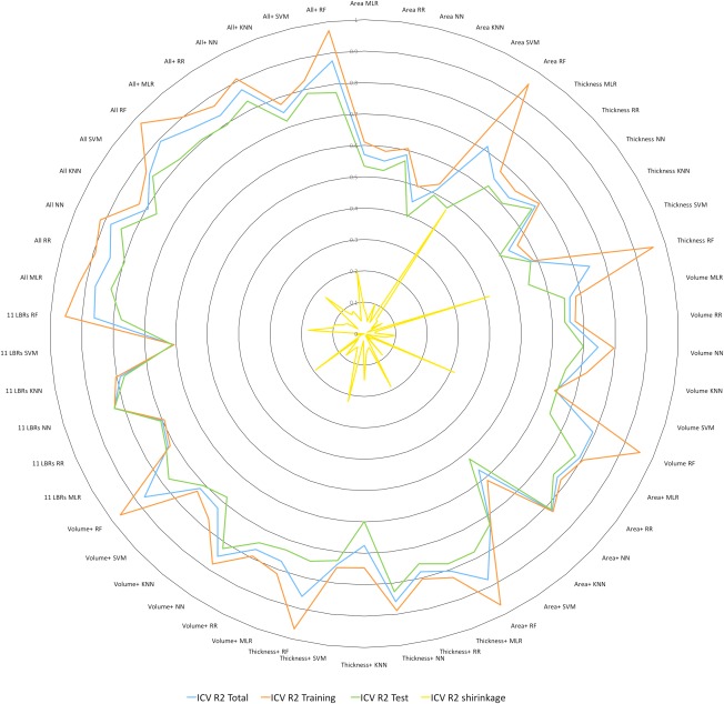
Radar plot showing all R ² values for all anatomical feature sets and methods (blue: R ² for the entire sample, green: R ² for the training sample, red: R ² for the test sample, black: R ² shrinkage between training and test). NN: neural network, RR: ridge regression, RF: random forest, MLR: multiple linear regression, KNN: k‐nearest neighbor.

Table 3.

Mean, minimum, and maximum R ² values (from the test sample) obtained for the six prediction methods

Method	Mean	Minimum	Maximum
NN	0.77	0.57	0.84
MLR	0.72	0.53	0.82
RF	0.70	0.48	0.81
RR	0.70	0.52	0.80
SVM	0.68	0.49	0.84
KNN	0.62	0.40	0.77

The R ² values are rank ordered for the mean R ² values.

Figure 2 shows the absolute prediction errors (absolute difference between predicted and chronological age) broken down for age, the different methods, and datasets. As one can see from these figures the absolute prediction error increases with increasing age.

Figure 2.

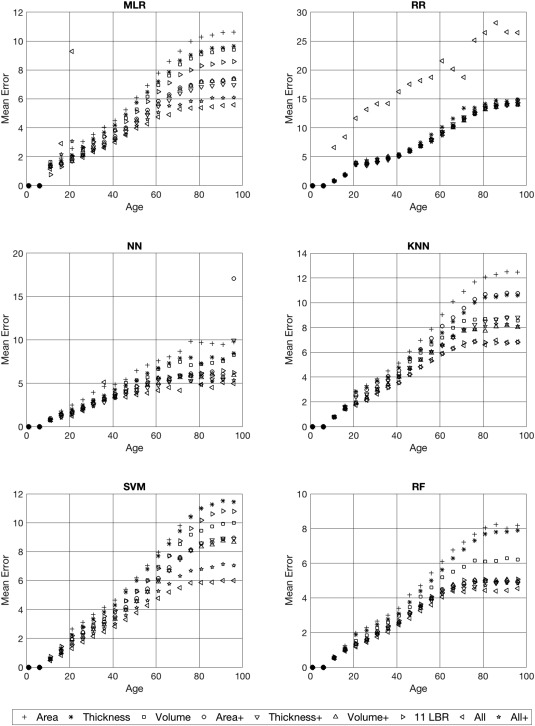
Absolute prediction errors broken down for the 6 different prediction techniques, the nine different anatomical feature sets, and age. The different anatomical feature sets are indicated as symbols in the graphs.

Table 4 shows mean prediction errors broken down for three age groups (8–18, 18–65, and 65–96 years). This Table reveals that depending on the used prediction method the absolute prediction error varies considerably. There are relatively small prediction errors for ALL and ALL+ feature set with an error of 1.23 years for the young subjects (8–18 years) obtained for the NN technique. This error increases to 4.23 and 5.23 years for the middle‐aged (18–65 years) and older subjects (65–96 years), respectively. The prediction errors obtained with the other techniques are a bit higher.

Table 4.

Mean absolute prediction errors broken down for the six different prediction techniques, the nine different anatomical feature sets, and three age‐groups

Methods		MLR		RR		NN		KNN		SVM		RF
Datasets	Age	M	SD	M	SD	M	SD	M	SD	M	SD	M	SD
Area	8–18	1.99	1.69	2.48	1.97	2.07	1.46	2.07	1.47	1.78	1.61	1.43	1.21
	18–65	8.38	6.50	10.23	9.40	8.14	6.94	9.76	7.36	8.68	8.56	6.61	6.47
	65–96	10.62	8.34	14.64	12.85	9.77	9.26	12.48	8.88	11.45	9.75	8.17	7.81
Thickness	8–18	1.67	1.62	2.32	1.72	1.48	1.21	1.98	1.62	1.59	1.27	1.34	1.22
	18–65	7.74	6.01	11.30	7.22	7.06	6.18	8.20	7.91	8.42	8.74	5.99	6.20
	65–96	9.64	7.27	14.91	10.99	8.46	7.26	10.59	9.80	11.45	10.62	7.90	7.76
Volume	8–18	1.88	1.93	2.58	2.14	1.57	1.29	1.57	1.26	1.38	1.37	1.15	1.08
	18–65	7.45	5.81	10.16	9.09	7.03	6.30	8.01	6.24	7.48	7.36	5.43	5.48
	65–96	9.40	7.12	14.01	13.45	8.28	7.42	8.57	7.73	9.98	8.21	6.21	6.99
Area+	8–18	1.63	1.63	2.31	1.66	1.78	1.42	1.96	1.43	1.43	1.23	1.08	1.06
	18–65	6.16	4.85	10.39	7.95	5.52	4.97	8.83	6.77	6.71	7.06	4.69	5.15
	65–96	7.41	5.53	14.82	10.74	17.06	10.98	10.75	8.09	8.94	8.02	4.93	5.56
Thickness+	8–18	1.29	1.28	2.31	1.66	1.46	1.13	1.92	1.60	1.33	1.11	1.09	1.05
	18–65	5.82	4.77	10.22	7.81	5.08	4.67	6.97	6.92	6.58	7.03	4.35	4.90
	65–96	6.97	5.62	14.23	11.56	9.95	15.28	8.81	8.17	8.90	8.30	4.90	5.72
Volume+	8–18	1.59	1.70	2.50	2.07	1.23	1.17	1.54	1.29	1.24	1.22	1.12	1.08
	18–65	6.07	5.03	9.78	8.97	5.02	4.84	6.96	6.18	6.49	6.65	4.53	5.17
	65–96	7.36	5.86	13.98	12.73	5.90	5.27	8.00	7.06	8.66	7.18	4.96	5.65
11 LBR	8–18	1.47	1.06	2.37	1.68	1.44	1.21	1.65	1.27	1.68	1.26	1.11	1.01
	18–65	6.98	5.56	10.03	8.72	5.55	5.58	6.20	6.11	7.54	8.20	4.70	5.20
	65–96	8.58	6.34	14.29	12.52	6.21	6.38	6.81	6.63	10.79	10.81	5.08	5.49
All	8–18	2.84	4.16	9.53	2.69	1.23	1.02	1.55	1.27	0.99	1.03	1.02	0.96
	18–65	5.03	4.25	14.57	12.35	4.50	4.22	6.23	5.71	5.15	4.72	4.18	4.63
	65–96	5.59	4.94	26.46	17.88	4.97	4.64	6.84	6.21	6.01	5.06	4.54	5.16
All+	8–18	5.48	7.94	2.26	1.65	1.42	1.57	1.62	1.32	1.14	1.16	1.11	1.00
	18–65	5.33	4.40	9.68	8.73	4.35	4.90	7.09	6.02	5.65	5.34	4.49	4.88
	65–96	6.10	4.95	13.94	12.00	5.35	5.05	8.10	7.08	7.04	5.93	4.84	5.65

DISCUSSION

With the current study we aimed at predicting chronological age on the basis of a combination of brain anatomical measures. Linked to this overall rationale, we were interested to answer different sub‐questions. First, we wanted to clarify which combination of anatomical measures is most suitable to predict age. Secondly, we explored whether a successful age prediction relies on a fine‐grained extraction of anatomical measures from many small brain regions, or whether it is sufficient to use brain measures from larger brain regions. Thirdly, we compared different statistical techniques with respect to their prediction accuracy. In the following paragraphs, we will discuss our findings and relate them to the current literature.

The main finding of our study is that age can be predicted with a high accuracy on the basis of anatomical measures. We identified 33 predictions with accuracies being larger than R ² = 0.70 with the highest accuracy of R ² =0.84. Thus, the prediction accuracy is in the same range (or even better) as has been demonstrated by previous studies using different anatomical measures and statistical prediction methods (R ²s ranging between 0.49 and 0.91) [Ashburner, 2007; Franke et al., 2013; Franke et al., 2012; Franke et al., 2014; Franke et al., 2010; Lao et al., 2004; Neeb et al., 2006]. However, different from the afore‐mentioned studies, we used a much larger sample (n > 3,400) spanning a large age range (7–96 years), and we used different sets of anatomical measures (thickness, volume, surface area).

Most astonishing was the finding that very good prediction accuracy was achieved even when using a small set of anatomical measures comprising only 11 larger brain regions with averaged anatomical characteristics across larger brain regions (e.g., grey and white matter volume, and cortical thickness, volume and area: 11 LBR). With this set of anatomical measures, we achieved a good prediction accuracy of R ² = 0.83 using the NN technique. The lowest prediction accuracy for this set of anatomical measures was obtained using the SVM technique (R ² = 0.61). Linear regression and RR revealed also reasonable results (R ² = 0.73 and R ² = 0.70, respectively).

The best prediction accuracy obtained with this reduced feature set only marginally differed from the best prediction accuracy achieved with a more fine‐grained feature set (R ² = 0.84 for the ALL dataset using NN or SVM, and R ² = 0.83 for the 11 LBR dataset using NN). Thus, it is clearly not necessary to use a large and sophisticated set of anatomical measures comprising very small brain areas to achieve accurate age prediction. The brain regions used for the 11 LBR dataset comprised relatively large brain compartments taken from the cortex, brainstem, and the cerebellum (cortical volume, cortical thickness, cortical area, cortical gray matter volume, cortical white matter volume, cerebellar gray matter volume, cerebellar white matter volume, subcortical volume, brainstem volume, corpus callosum, white matter hypo‐intensities). Thus, a combination of these different cortical, sub‐cortical and cerebellar brain measures are at least as effective for predicting age than larger datasets comprising relatively small cortical measures.

That the anatomical dataset with the large cortical, subcortical and cerebellar volume LBRs are so useful for predicting age might result from the fact that age effects on brain anatomy are mostly distributed and not focal. Several recent studies have shown that older subjects demonstrate smaller volumes in many distributed cortical, subcortical and cerebellar regions [Fjell et al., 2009a; Fjell et al., 2009b; Jäncke et al., 2015; Tang et al., 2013; Ziegler et al., 2012]. As cortical volumes become smaller with increasing age, cerebrospinal fluid and white matter T1‐weighted hypo‐intensity (T2‐weighted hyper‐intensity) volumes increase. Thus, combining volume measures from these different brain regions seems to be a good and valid strategy for capturing age‐related anatomical differences more accurately and efficiently.

In this study, we used six different statistical techniques for age prediction. It turned out that the accuracy of these methods is mostly depended on the dataset. However, the KNN method had the weakest results overall, with an average accuracy of R ² = 0.62. Each of the techniques used provide different advantages and disadvantages, which should be carefully taken into consideration when planning to predict age on the basis of anatomical measures.

The MLR approach is a standard statistical technique frequently used in psychology and neuroscience. It is relatively easy to program and can be run quickly even with a large number of predictor variables. However, a problematic aspect is the possibility of correlated predictors, which can distort the prediction accuracy substantially (e.g., suppression effects) [Pedhazur, 1997]. In addition, in order to achieve reasonably good prediction accuracies, it is necessary to use large samples for the training, a prerequisite that was easily met by our sample with 3,144 participants. In our study, the MLR technique revealed very good results for nearly all datasets, with the exception of AREA and THICKNESS.

Similar to the MLR technique, RR is simple to program, runs quickly (even a bit faster than MLR) and can be used in so‐called ill‐defined mathematical conditions and when too many predictors are used. For example, when it is impossible to calculate an inverse matrix (a mathematical operation, which is necessary to calculate linear regressions), RR is a suitable solution [Hoerl & Kennard, 1970]. Nevertheless, possible statistical dependencies between the predictors can distort the prediction results, similar to the MLR technique. For our dataset, RR revealed similar results to the MLR technique.

The NN approach is a bit more complicated to implement in terms of programming effort. It is a time‐ and resource‐consuming technique, and requires large sample sizes. It can, however, handle many correlated predictors as well as linear and non‐linear relationships without any a priori knowledge about the relationships. In our study, the NN approach provided the best results with small R ² shrinkages, although it must be kept in mind that the differences to the other techniques are quite small. Nevertheless, out of our nine datasets, NN provided the best results for eight datasets.

The KNN approach is a time‐consuming technique with some similarities to the NN technique. The precision of this technique is highly dependent on the predictors used, as has been shown by our study. KNN revealed mixed results in our study, with only one good result for the 11 LBR dataset that was in the same range as the NN results. For all other datasets, KNN had moderate or weak predictive power.

The SVM technique is a bit more demanding to implement, but is relatively fast and provides stable results. Similar to the KNN, the results strongly depend on the selection of predictors. The results in our study were roughly similar to those from the NN technique. SVM provided good results only when large datasets were used (ALL and ALL+).

The RF technique is a very time‐consuming technique that can handle correlated predictors, requires only small learning sets and is less affected by correlated predictors. Similar to the KNN and NN approaches, the results strongly depend on the selection of predictors used. For our data, RF revealed similar results to the MLR technique.

To summarize our findings with respect to the precision of the techniques used, NN provided the best results across all datasets, irrespective of whether they comprised only a few or many anatomical measures. However, the relatively simple and widely used MLR technique also provided good results. Since RR is nearly as good as MLR, it can be used in mathematically problematic situations. RF, although providing reasonable results, is too time consuming and it offers no added gains.

The absolute prediction errors (difference between predicted and chronological age) we obtained in our analyses are quite similar to those reported in previous studies [Brown et al., 2012; Cherubini et al., 2016; Franke et al., 2010]. However, it is worth mentioning that our study cannot be compared entirely with these studies, either because they only studied relatively young subjects [Brown et al., 2012] or they employed a much smaller sample than we used in our study [Cherubini et al., 2016]. However, the results are astonishingly similar in showing that the prediction error increases with increasing age [Brown et al., 2012; Franke et al., 2010]. In addition, the prediction errors in our study are about in same range as it was reported in these studies, at least for the methods and datasets for which we achieved good and very good prediction results.

CONCLUSION

Taken together, the results of the present study demonstrate that chronological age can be predicted quite well on the basis of anatomical measures. The NN approach revealed to be the approach with the best prediction accuracy. In addition, it was evident that good prediction accuracies can be achieved using a reduced, but nevertheless age‐representative dataset (e.g., 11 LBR).

Supporting information

Supporting Information

Supporting Information

REFERENCES

- Ashburner J (2007): A fast diffeomorphic image registration algorithm. Neuroimage 95–113. [DOI] [PubMed] [Google Scholar]
- Basak D, Pal S, Patranabis DC (2007): Support vector regression. Neural Inform Process‐Lett Rev 11:203–224. [Google Scholar]
- Battiti R (1992): First‐and second‐order methods for learning: Between steepest descent and Newton's method. Neural Computation 4:141–166. [Google Scholar]
- Bezzola L, Merillat S, Gaser C, Jancke L (2011): Training‐induced neural plasticity in golf novices. J Neurosci 31:12444–12448. [DOI] [PMC free article] [PubMed] [Google Scholar]
- Breiman L (2001): Random forests. Machine Learn 45:5–32. [Google Scholar]
- Brown TT, Kuperman JM, Chung Y, Erhart M, McCabe C, Hagler DJ Jr, Venkatraman VK, Akshoomoff N, Amaral DG, Bloss CS, Casey BJ, Chang L, Ernst TM, Frazier JA, Gruen JR, Kaufmann WE, Kenet T, Kennedy DN, Murray SS, Sowell ER, Jernigan TL, Dale AM (2012): Neuroanatomical assessment of biological maturity. Curr Biol 22:1693–1698. [DOI] [PMC free article] [PubMed] [Google Scholar]
- Burba F, Ferraty F, Vieu P (2009): k‐Nearest Neighbour method in functional nonparametric regression. J Nonparametric Stat 21:453–469. [Google Scholar]
- Castro E, Gómez‐Verdejo V, Martínez‐Ramón M, Kiehl K, Calhoun V (2014): A multiple kernel learning approach to perform classification of groups from complex‐valued fMRI data analysis: Application to schizophrenia. Neuroimage 87:1–17. [DOI] [PMC free article] [PubMed] [Google Scholar]
- Cherubini A, Caligiuri ME, Peran P, Sabatini U, Cosentino C, Amato F (2016): Importance of multimodal MRI in characterizing brain tissue and its potential application for individual age prediction. IEEE J Biomed Health Inform [DOI] [PubMed] [Google Scholar]
- Cohen J (1992): A power primer. Psychol Bull 112:155–159. [DOI] [PubMed] [Google Scholar]
- Dai D, Wang J, Hua J, He H (2012): Classification of ADHD children through multimodal magnetic resonance imaging. Front Syst Neurosci 6:63. [DOI] [PMC free article] [PubMed] [Google Scholar]
- Dall'Acqua P, Johannes S, Mica L, Simmen HP, Glaab R, Fandino J, Schwendinger M, Meier C, Ulbrich EJ, Muller A, Jancke L, Hanggi J (2016): Connectomic and surface‐based morphometric correlates of acute mild traumatic brain injury. Front Hum Neurosci 10:127. [DOI] [PMC free article] [PubMed] [Google Scholar]
- de Bruin E, Hulshoff Pol H, Bijl S, Schnack H, Fluitman S, Bocker K, Kenemans J, Kahn R, Verbaten M (2005): Associations between alcohol intake and brain volumes in male and female moderate drinkers. Alcohol. Clin Exp Res 29:656–663. [DOI] [PubMed] [Google Scholar]
- Destrieux C, Fischl B, Dale A, Halgren E (2010): Automatic parcellation of human cortical gyri and sulci using standard anatomical nomenclature. Neuroimage 53:1–15. [DOI] [PMC free article] [PubMed] [Google Scholar]
- Fan Y, Batmanghelich N, Clark C, Davatzikos C, Alzheimer's DNI (2008): Spatial patterns of brain atrophy in MCI patients, identified via high‐dimensional pattern classification, predict subsequent cognitive decline. Neuroimage 39:1731–1743. [DOI] [PMC free article] [PubMed] [Google Scholar]
- Fischl B, Salat D, van der Kouwe A, Makris N, Segonne F, Quinn B, Dale A (2004a): Sequence‐independent segmentation of magnetic resonance images. Neuroimage 23Suppl1:S69–S84. [DOI] [PubMed] [Google Scholar]
- Fischl B, van der Kouwe A, Destrieux C, Halgren E, Segonne F, Salat D, Busa E, Seidman L, Goldstein J, Kennedy D, Caviness V, Makris N, Rosen B, Dale A (2004b): Automatically parcellating the human cerebral cortex. Cereb Cortex 14:11–22. [DOI] [PubMed] [Google Scholar]
- Fjell A, Walhovd K (2010): Structural brain changes in aging: Courses, causes and cognitive consequences. Rev Neurosci 21:187–221. [DOI] [PubMed] [Google Scholar]
- Fjell A, Westlye L, Amlien I, Espeseth T, Reinvang I, Raz N, Agartz I, Salat D, Greve D, Fischl B, Dale A, Walhovd K (2009a): Minute effects of sex on the aging brain: A multisample magnetic resonance imaging study of healthy aging and Alzheimer's disease. J Neurosci 29:8774–8783. [DOI] [PMC free article] [PubMed] [Google Scholar]
- Fjell AM, Westlye LT, Amlien I, Espeseth T, Reinvang I, Raz N, Agartz I, Salat DH, Greve DN, Fischl B, Dale AM, Walhovd KB (2009b): High consistency of regional cortical thinning in aging across multiple samples. Cereb Cortex 19:2001–2012. [DOI] [PMC free article] [PubMed] [Google Scholar]
- Franke K, Ziegler G, Klöppel S, Gaser C, Alzheimer's DNI (2010): Estimating the age of healthy subjects from T1‐weighted MRI scans using kernel methods: Exploring the influence of various parameters. Neuroimage 50:883–892. [DOI] [PubMed] [Google Scholar]
- Franke K, Luders E, May A, Wilke M, Gaser C (2012): Brain maturation: Predicting individual BrainAGE in children and adolescents using structural MRI. Neuroimage 63:1305–1312. [DOI] [PubMed] [Google Scholar]
- Franke K, Gaser C, Manor B, Novak V (2013): Advanced BrainAGE in older adults with type 2 diabetes mellitus. Front Aging Neurosci 5:90. [DOI] [PMC free article] [PubMed] [Google Scholar]
- Franke K, Ristow M, Gaser C, Alzheimer's DNI (2014): Gender‐specific impact of personal health parameters on individual brain aging in cognitively unimpaired elderly subjects. Front Aging Neurosci 6:94. [DOI] [PMC free article] [PubMed] [Google Scholar]
- Franke K, Hagemann G, Schleussner E, Gaser C (2015): Changes of individual BrainAGE during the course of the menstrual cycle. Neuroimage 115:1–6. [DOI] [PubMed] [Google Scholar]
- Gaser C, Franke K, Klöppel S, Koutsouleris N, Sauer H, Alzheimer's DNI (2013): BrainAGE in mild cognitive impaired patients: Predicting the conversion to Alzheimer's disease. PLoS One 8:e67346. [DOI] [PMC free article] [PubMed] [Google Scholar]
- Hilti LM, Hanggi J, Vitacco DA, Kraemer B, Palla A, Luechinger R, Jancke L, Brugger P (2013): The desire for healthy limb amputation: structural brain correlates and clinical features of xenomelia. Brain 136:318–329. [DOI] [PubMed] [Google Scholar]
- Hinrichs C, Singh V, Mukherjee L, Xu G, Chung M, Johnson S, Alzheimer's DNI (2009): Spatially augmented LPboosting for AD classification with evaluations on the ADNI dataset. Neuroimage 48:138–149. [DOI] [PMC free article] [PubMed] [Google Scholar]
- Hinrichs C, Singh V, Xu G, Johnson S, Alzheimers DNI (2011): Predictive markers for AD in a multi‐modality framework: An analysis of MCI progression in the ADNI population. Neuroimage 55:574–589. [DOI] [PMC free article] [PubMed] [Google Scholar]
- Hoerl AE, Kennard RW (1970): Ridge regression: Biased estimation for nonorthogonal problems. Technometrics 12:55–67. [Google Scholar]
- Jäncke L, Mérillat S, Liem F, Hänggi J (2015): Brain size, sex, and the aging brain. Hum Brain Mapp 36:150–169. [DOI] [PMC free article] [PubMed] [Google Scholar]
- Kasparek T, Thomaz C, Sato J, Schwarz D, Janousova E, Marecek R, Prikryl R, Vanicek J, Fujita A, Ceskova E (2011): Maximum‐uncertainty linear discrimination analysis of first‐episode schizophrenia subjects. Psychiatry Res 191:174–181. [DOI] [PubMed] [Google Scholar]
- Klauschen F, Goldman A, Barra V, Meyer‐Lindenberg A, Lundervold A (2009): Evaluation of automated brain MR image segmentation and volumetry methods. Hum Brain Mapp 30:1310–1327. [DOI] [PMC free article] [PubMed] [Google Scholar]
- Klein C, Hanggi J, Luechinger R, Jancke L (2015): MRI with and without a high‐density EEG cap‐‐what makes the difference? Neuroimage 106:189–197. [DOI] [PubMed] [Google Scholar]
- Klöppel S, Abdulkadir A, Jack C, Koutsouleris N, Mourão‐Miranda J, Vemuri P (2012): Diagnostic neuroimaging across diseases. Neuroimage 61:457–463. [DOI] [PMC free article] [PubMed] [Google Scholar]
- Langer N, Pedroni A, Gianotti LR, Hanggi J, Knoch D, Jancke L (2012): Functional brain network efficiency predicts intelligence. Hum Brain Mapp 33:1393–1406. [DOI] [PMC free article] [PubMed] [Google Scholar]
- Lao Z, Shen D, Xue Z, Karacali B, Resnick S, Davatzikos C (2004): Morphological classification of brains via high‐dimensional shape transformations and machine learning methods. Neuroimage 21:46–57. [DOI] [PubMed] [Google Scholar]
- Leonard C, Kuldau J, Breier J, Zuffante P, Gautier E, Heron D, Lavery E, Packing J, Williams S, DeBose C (1999): Cumulative effect of anatomical risk factors for schizophrenia: An MRI study. Biol Psychiatry p 374–382. [DOI] [PubMed] [Google Scholar]
- Li W, van Tol MJ, Li M, Miao W, Jiao Y, Heinze HJ, Bogerts B, He H, Walter M (2014): Regional specificity of sex effects on subcortical volumes across the lifespan in healthy aging. Hum Brain Mapp 35:238–247. [DOI] [PMC free article] [PubMed] [Google Scholar]
- Mondadori CR, de Quervain DJ, Buchmann A, Mustovic H, Wollmer MA, Schmidt CF, Boesiger P, Hock C, Nitsch RM, Papassotiropoulos A, Henke K (2007): Better memory and neural efficiency in young apolipoprotein E epsilon4 carriers. Cereb Cortex 17:1934–1947. [DOI] [PubMed] [Google Scholar]
- Nakamura K, Kawasaki Y, Suzuki M, Hagino H, Kurokawa K, Takahashi T, Niu L, Matsui M, Seto H, Kurachi M (2004): Multiple structural brain measures obtained by three‐dimensional magnetic resonance imaging to distinguish between schizophrenia patients and normal subjects. Schizophr Bull 30:393–404. [DOI] [PubMed] [Google Scholar]
- Neeb H, Zilles K, Shah N (2006): Fully‐automated detection of cerebral water content changes: Study of age‐ and gender‐related H2O patterns with quantitative MRI. Neuroimage 29:910–922. [DOI] [PubMed] [Google Scholar]
- Pannacciulli N, Del Parigi A, Chen K, Le D, Reiman E, Tataranni P (2006): Brain abnormalities in human obesity: A voxel‐based morphometric study. Neuroimage 31:1419–1425. [DOI] [PubMed] [Google Scholar]
- Pedhazur EJ (1997) Multiple Regression in Behavioral Research. Wadsworth Publishing Co Inc; p 1072. [Google Scholar]
- Sato J, Hoexter M, Fujita A, Rohde L (2012): Evaluation of pattern recognition and feature extraction methods in ADHD prediction. Front Syst Neurosci 6:68. [DOI] [PMC free article] [PubMed] [Google Scholar]
- Schnack H, Nieuwenhuis M, van Haren N, Abramovic L, Scheewe T, Brouwer R, Hulshoff Pol H, Kahn R (2014): Can structural MRI aid in clinical classification? A machine learning study in two independent samples of patients with schizophrenia, bipolar disorder and healthy subjects. Neuroimage 299–306. [DOI] [PubMed] [Google Scholar]
- Seidman L, Valera E, Bush G (2004): Brain function and structure in adults with attention‐deficit/hyperactivity disorder. Psychiatr Clin North Am 27:323–347. [DOI] [PubMed] [Google Scholar]
- Strobl C, Malley J, Tutz G (2009): An introduction to recursive partitioning: Rationale, application, and characteristics of classification and regression trees, bagging, and random forests. Psychol Methods 14:323–348. [DOI] [PMC free article] [PubMed] [Google Scholar]
- Takayanagi Y, Takahashi T, Orikabe L, Mozue Y, Kawasaki Y, Nakamura K, Sato Y, Itokawa M, Yamasue H, Kasai K, Kurachi M, Okazaki Y, Suzuki M (2011): Classification of first‐episode schizophrenia patients and healthy subjects by automated MRI measures of regional brain volume and cortical thickness. PLoS One 6:e21047. [DOI] [PMC free article] [PubMed] [Google Scholar]
- Taki Y, Goto R, Evans A, Zijdenbos A, Neelin P, Lerch J, Sato K, Ono S, Kinomura S, Nakagawa M, Sugiura M, Watanabe J, Kawashima R, Fukuda H (2004): Voxel‐based morphometry of human brain with age and cerebrovascular risk factors. Neurobiol Aging 25:455–463. [DOI] [PubMed] [Google Scholar]
- Taki Y, Kinomura S, Sato K, Goto R, Inoue K, Okada K, Ono S, Kawashima R, Fukuda H (2006): Both global gray matter volume and regional gray matter volume negatively correlate with lifetime alcohol intake in non‐alcohol‐dependent Japanese men: A volumetric analysis and a voxel‐based morphometry. Alcohol Clin Exp Res 30:1045–1050. [DOI] [PubMed] [Google Scholar]
- Tang T, Jiao Y, Wang X, Lu Z (2013): Gender versus brain size effects on subcortical gray matter volumes in the human brain. Neurosci Lett 1–5. [DOI] [PubMed] [Google Scholar]
- Wachinger C, Golland P, Kremen W, Fischl B, Reuter M, Alzheimer's DNI (2015): BrainPrint: A discriminative characterization of brain morphology. Neuroimage 109:232–248. [DOI] [PMC free article] [PubMed] [Google Scholar]
- Wachinger C, Golland P, Reuter M (2014): BrainPrint: Identifying subjects by their brain. Med Image Comput Comput Assist Interv 17:41–48. [DOI] [PMC free article] [PubMed] [Google Scholar]
- Ziegler G, Dahnke R, Jancke L, Yotter R, May A, Gaser C (2012): Brain structural trajectories over the adult lifespan. Hum Brain Mapp 33:2377–2389. [DOI] [PMC free article] [PubMed] [Google Scholar]
Associated Data
This section collects any data citations, data availability statements, or supplementary materials included in this article.
Supplementary Materials