Comparison of a non‐stationary voxelation‐corrected cluster‐size test with TFCE for group‐Level MRI inference

Abstract

Two powerful methods for statistical inference on MRI brain images have been proposed recently, a non‐stationary voxelation‐corrected cluster‐size test (CST) based on random field theory and threshold‐free cluster enhancement (TFCE) based on calculating the level of local support for a cluster, then using permutation testing for inference. Unlike other statistical approaches, these two methods do not rest on the assumptions of a uniform and high degree of spatial smoothness of the statistic image. Thus, they are strongly recommended for group‐level fMRI analysis compared to other statistical methods. In this work, the non‐stationary voxelation‐corrected CST and TFCE methods for group‐level analysis were evaluated for both stationary and non‐stationary images under varying smoothness levels, degrees of freedom and signal to noise ratios. Our results suggest that, both methods provide adequate control for the number of voxel‐wise statistical tests being performed during inference on fMRI data and they are both superior to current CSTs implemented in popular MRI data analysis software packages. However, TFCE is more sensitive and stable for group‐level analysis of VBM data. Thus, the voxelation‐corrected CST approach may confer some advantages by being computationally less demanding for fMRI data analysis than TFCE with permutation testing and by also being applicable for single‐subject fMRI analyses, while the TFCE approach is advantageous for VBM data. Hum Brain Mapp 38:1269–1280, 2017. © 2016 Wiley Periodicals, Inc.

Abbreviations

AFROC

Alternative FROC

CDT

Cluster‐defining threshold

CST

Cluster‐size test

FDR

False discovery rate

FWE

Family‐wise error

fMRI

Functional magnetic resonance imaging

FROC

Free‐response receiver‐operator characteristic

NC

Normal control

RESEL

Resolution element

RFT

Random field theory

ROC

Receiver‐operator characteristic

RPV

RESELs per voxel

SNR

Signal to noise ratio

TBSS

Tract‐based spatial statistic

TFCE

Threshold‐free cluster enhancement

VBM

Voxel‐based morphometry

vn‐CST

Voxelation‐corrected cluster‐size test

INTRODUCTION

Accurately determining the significance of changes (i.e., activations) in brain images is one of the most critical procedures of functional neuroimaging. However, this entails conducting statistical tests over tens of thousands of voxels, which presents a problem for controlling the number of false positives. Many approaches correcting for multiple tests have been proposed for inference on brain maps. The most widely used approaches are based on family‐wise error (FWE) correction [Cao and Worsley, 2001; Friston et al., 1994; Forman et al., 1995; Nichols and Holmes, 2002; Worsley et al., 1996]. An alternative to FWE correction is false discovery rate (FDR) correction based on controlling the expected proportion of rejected hypotheses that are false positives [Benjamini and Heller, 2007; Chumbley and Friston, 2009; Chumbley et al., 2009; Genovese et al., 2002]. Although FDR is potentially more powerful, it is not yet as widely used as FWE corrections.

Among the methods based on FWE correction, there are two cluster‐size based approaches which do not place constraints on the spatial smoothness of the images: the non‐stationary voxelation‐corrected cluster‐size test (vn‐CST) based on selecting a cluster‐defining threshold (CDT) to identify activation clusters, combined with random field theory (RFT) for inference [Li et al., 2015], and threshold‐free cluster enhancement [TFCE; Smith and Nichols, 2009] based on estimating a voxel‐wise metric that captures the amount of cluster‐like local spatial support for an activation, combined with non‐parametric permutation testing for inference [Hayasaka et al., 2004; Holmes et al., 1996; Nichols and Holmes, 2002]. Since neither of these approaches require high degrees of spatial smoothness and/or uniform spatial smoothness, they are both ideal for high spatial resolution MRI data, e.g., voxel‐based morphometry (VBM) data or tract‐based spatial statistic (TBSS) images to localize brain changes related to development, degeneration and disease.

The vn‐CST is based on extending the formulation of a recently proposed method, the voxelation‐corrected CST (v‐CST) based on Gaussian Random Field (GRF) theory [Li et al., 2014], to RFT [Li et al., 2015]. Unlike other CST methods based on GRF or RFT, which can only be used to control FWE when the image is highly spatial smoothed [Hayasaka and Nichols, 2003; Li et al., 2014, 2015], v‐CST and vn‐CST are suitable for analyzing images without a high degree of spatial smoothness. The improvement with v‐ and vn‐CST is achieved by adjusting the smoothness estimator of the statistical parametric map to take into account the effects of voxelation when the spatial smoothness is comparable to the voxel size. vn‐CST goes one step further than v‐CST by extending the framework from GRF to RFT, and, compared to v‐CST, vn‐CST is a more reliable and effective for controlling FWE in images with non‐uniform spatial smoothness. Notably, vn‐CST is applicable for both stationary and non‐stationary images and performs better under low spatial smoothness and low degrees of freedom (dfs) when compared to the widely used original non‐stationary CST [Worsley et al., 1999; Worsley, 2002], which requires images with high degrees of spatial smoothness and large dfs [Silver et al., 2011].

Recent work by Eklund et al. [2016] showed that standard CSTs based on RFT implemented in FSL and SPM produced invalid FWE at typical CDTs, and that non‐stationarity in functional magnetic resonance imaging (fMRI) data could be a contributor to the invalid performance of these approaches. Notably, they also found that the original non‐stationary CST based on RFT implemented in the non‐stationary toolbox for SPM also produced invalid FWE at tested CDTs. Our vn‐CST approach has great potential to obviate some of these issues for inference on brain maps and represents a more robust alternative to currently implemented cluster‐based RFT methods.

The TFCE approach takes a raw statistic image and produces an output image in which the voxel‐wise values represent the amount of cluster‐like local spatial support by combining spatially distributed cluster size and height information. The output value is therefore a weighted sum of the entire local clustered signal. For inference, voxel‐level permutation testing is used to turn the TFCE image into voxel‐wise P‐values. Notably, TFCE avoids an arbitrary choice of CDT, has no requirements for spatial smoothing and is relatively unaffected by non‐stationarity [Salimi‐Khorshidi et al., 2011 ; Smith and Nichols, 2009]. Thus, this method retains the sensitivity of cluster‐based approaches without the need for a hard cluster‐forming threshold. Unlike CST approaches based on GRF or RFT (which are parametric), the distribution of the TFCE statistic is not known, necessitating the use of non‐parametric permutation testing for inference on the TFCE statistic maps at the group level. For individual subject‐level fMRI analysis, no clear‐cut approach for inference on the TFCE statistic maps is available because fMRI timepoints in a timeseries are not exchangeable, which is a requirement for non‐parametric permutation testing [although there has been some limited work to develop approaches that obviate this issue (Zhou and Wang, 2009)]. Thus, for single‐subject fMRI data analysis, v‐CST and vn‐CST may be more attractive approaches.

For group‐level fMRI data analysis, the TFCE approach outperforms the original stationary and non‐stationary CST inference approaches based on RFT [Salimi‐Khorshidi et al., 2011; Smith and Nichols, 2009]. In addition, our recent work showed a clear advantage of vn‐CST over the original CST and over our proposed v‐CST [Li et al., 2015]. However, there are no studies comparing the performance of vn‐CST and TFCE for group‐level analysis. In this work, we are concerned with group‐level inference; namely, we investigate the effectiveness of vn‐CST and TFCE under different dfs, smoothness levels and signal to noise ratios (SNRs) for both stationary and non‐stationary images for group‐level analysis. Simulated null data and simulated activation data were used to generate stationary and non‐stationary data to test the techniques under know conditions.

MATERIALS AND METHODS

Description of Inference Methods

Non‐stationary voxelation‐corrected cluster‐size test

The vn‐CST retains high sensitivity without requiring high and uniform image smoothing mainly through: the modification of the mathematical model for estimating image local roughness and the correction for voxel size.

For vn‐CST, the estimate of local roughness of voxel location i, that takes into account the effect of voxel size, e.g., the voxelation‐corrected local roughness, can be expressed as, Λ_ic [Li et al., 2014]:

$$|{\Lambda }_{ic}|=\left(\frac{2{|{\Lambda }_i|}^{1/3}}{2+{|{\Lambda }_i|}^{1/3}}\right)$$ (1)

Λ_i is the uncorrected local roughness of voxel location i, which can be derived from the spatial derivatives of multiple residual images at every voxel [Kiebel et al., 1999].

The voxel size for vn‐CST is given in the units of resolution element (RESEL), e.g., RESELs per voxel (RPV), which is an extension of the RPV from Worsley et al. [1999] that uses Λ_ic instead of Λ_i:

$$RP{V}_{ic}={(4\log 2)}^{-3/2}{|{\Lambda }_{ic}|}^{1/2}$$ (2)

The cluster size k is calculated by summing up the RPV_ic within each cluster [Li et al., 2015]:

$$k={\displaystyle \sum _{i\in C}RP{V}_{ic}}$$ (3)

The uncorrected cluster‐size distribution ‐ the distribution of a single cluster size above a given CDT t‐value, for vn‐CST can be expressed as:

$$p(m\ge k)={\left(1+\frac{\sqrt{k\gamma }}{t^2}\right)}^2\exp \left(-\sqrt{k\gamma }-\frac{1}{2}\frac{k\gamma }{t^2}\right)$$ (4)

where $\gamma$ is a known parameter that has a relationship with the CDT that makes vn‐CST applicable for low CDT.

The FWE corrected probability of clusters with a specific size k or larger, searched over a brain region, and exceeding a given CDT t‐value, $p_r(m\ge k)$, can then be computed based on the Poisson clumping heuristic:

$$p_r(m\ge k)=1-\exp (-E(L)p(m\ge k))$$ (5)

where L is the number of clusters above t, $E(L)$ is the expected number of clusters [Worsley et al., 1996].

TFCE analysis and inference

Inference at the group level using the TFCE approach proceeds in two steps. First, the TFCE statistic is calculated for each voxel, i, in the input raw statistic image as the sum of the scores of all Supporting Information section underneath it, as follows:

$$TFCE(i)={\displaystyle {\int }_{h-h_0}^{h_i}e{(h)}^E{h}^{H}dh}$$ (6)

where E and H are tuning parameters set to recommended values of 0.5 and 2, respectively, for fMRI data and different values for, e.g., TBSS data [Smith and Nichols, 2009]. e(h) is the extent of the cluster that voxel i belongs to with cluster‐forming threshold h. Thus, in the output TFCE image, each voxel‐wise value represents the amount of cluster‐like local spatial support of the original signal at each voxel. While this method obviates setting a cluster‐forming threshold, the parameters E and H must still be set, although the default values have been shown to work well for a wide range of image characteristics [Smith and Nichols, 2009]. Once the TFCE image is computed for each subject, inference at the group‐level is achieved using non‐parametric permutation testing to calculate the FWE‐corrected P‐value at each voxel.

Evaluation Data Used

To estimate the effectiveness of vn‐CST and TFCE methods in controlling false positives for group‐level analysis, Monte‐Carlo simulations were used to generate both stationary and non‐stationary t random noise data (null data). The sensitivity of vn‐CST and TFCE methods was compared using simulated MRI data that were generated by adding realistic ground truth task activation signals and between group variations to null data, resting‐state fMRI (rfMRI) data, and structural MRI data.

Computer simulation study

Simulated null data

The Monte‐Carlo simulations used to generate both stationary and non‐stationary null data used a strategy similar to that implemented by Hayasaka et al. [2004]. For the null data simulations, 2,000 realizations were generated for two‐group data with three different sample sizes. For each realization, three sets of two‐group data were generated, with the number of subjects per group in a set fixed at 10, 20 and 30 subjects per group, with 64 x 64 x 32 Gaussian images, and a two‐sample t‐test was used to calculate the statistic images with df = 18, 38 and 58, respectively.

For the stationary null data simulation, we tested different levels of spatial smoothness by varying the applied (full width at half maximum) FWHM of the Gaussian kernel, with FWHM = 1.5, 3, 6 and 9 voxels. For the non‐stationary null data simulation, each white noise image was smoothed with three different 3D Gaussian kernels, producing three images with low, medium and high smoothness. These images were combined such that a central core smoothed with FWHM_c was encircled by a middle layer smoothed with FWHM_m, which was in turn encircled by an outer layer smoothed with FWHM_o. Six settings (FWHM_c/FWHM_m/FWHM_o: 0/1.5/3, 3/1.5/0, 3/4.5/6, 6/4.5/3, 5/4.5/4 and 7.5/4.5/1.5 voxels) were used to simulate different levels of non‐stationary data. The resulting non‐stationary image were also scaled to ensure that the variance of the noise was unity.

The significance level of the tests was set to 0.05, for which the normal approximation of the 95% confidence interval is 4.04%‐5.96%. Each test's rejection rate was calculated by taking the number of realizations that contained detected clusters divided by the total number of realizations. Unlike TFCE inference (which does not require an a priori threshold but does involve default TFCE height and extent parameters), the results of vn‐CST methods depend on the CDT. For vn‐CST, performance was tested with CDT t‐values = 2.5, 3.0, 3.5, 4.0 and 4.5 (these CDTs were used for all simulations in this work). Suprathreshold voxels were searched first and then clusters of suprathreshold voxels were identified with 18 connectivity algorithms. For the TFCE analysis, FSL Randomise (http://fsl.fMRIb.ox.ac.uk/fsl/fslwiki/Randomise) was used with default cluster parameters of H = 2 (power of cluster height) and E = 0.5 (power of cluster extent). The number of permutations was set to 1,000 with the default connectivity.

Simulated activation data

Simulated activation data were generated by constructing an activation signal for a two‐group analysis under conditions in which the ground truth spatial activation pattern is known. A mask with 20 clusters, with cluster sizes ranging from 2 to 502 voxels, was used as the ground truth spatial pattern (Table I). This spatial pattern was utilized to construct ground truth fMRI activation blobs embedded in the simulated null data. The ground truth fMRI signal had a background value of 0 and a peak value of 1.

Table I.

Cluster size (in voxels) of the ground truth activation regions for Monte Carlo simulation, rfMRI‐based and VBM‐based simulation

Monte Carlo simulation	508	318	315	306	193	167	132	109	86	85
	81	55	54	49	45	27	25	14	7	2
rfMRI‐based simulation	18545	178	102	86	85	57	55	45	27	15
VBM‐based simulation	2442	748	520	239	238	109	69	50	49	38
	34	30

For the simulated stationary task data, the signal data was first scaled by 1, 3 or 5, and then added to the simulated unsmoothed null data to give images with a range of peak SNR values = 1, 3 and 5, respectively. These unsmoothed stationary task data with different SNR levels were then spatially smoothed using FWHM = 1.5, 3, 6 and 9 voxels to generate data with different levels of SNR/smoothness over all SNR and FWHM values. For simulated non‐stationary activation data, the same concentric smoothing strategy (which was used to generate the simulated non‐stationary null data) was applied to the unsmoothed stationary task data (for all three SNRs).

For the activation data simulation, 20 realizations were generated for each sample size (df = 18, 38 and 58). For TFCE, FSL Randomise was used to estimate the between‐group difference and find the activation regions. The number of permutations was set to 5,000 with the default connectivity. Receiver‐operator characteristic (ROC) curves were used to compare performance of vn‐CST and TFCE. As discussed by Smith and Nichols. [2009], various TPR and FPR measures can be defined when multiple tests are considered. In this case, both free‐response receiver‐operator characteristic (FROC) and alternative FROC (AFROC) can be used. FROC plots the proportion of true positive tests versus the expected number of false positives per image. AFROC plots the proportion of true positive tests versus the probability of any false positive detection anywhere in the image. As neuroimaging analyses typically seek to control the FWE rate, we chose to use AFROC in our study [similar to Smith and Nichols, 2009]. With FWE‐false positive rate (FWE‐FPR) chosen as the x‐axis and the measured cluster‐wise true positive rate (TPR) (the number of detected true activation clusters divided by the total number of activation clusters) chosen as the y‐axis. Since only performance with low FPR is of interest, we compared ROC curves for FWE‐FPR < 0.05, and the corresponding AUC was scaled by 1/0.05 to renormalize the AUC to the range [0, 1]. The significance level of all tests was set to 0.05.

rfMRI‐based simulation

In this study, simulated ground truth task‐activation responses were added into high‐spatial and temporal resolution resting state data in prescribed regions of the brain (primarily visual cortex). High resolution rfMRI data (2 × 2 × 2 mm³ resolution acquired at 3T) were obtained from the HCP (http://www.humanconnectome.org/data/). Data from 20 unrelated subjects with minimal pre‐processing were downloaded. The acquisition protocol and pre‐processing pipelines have been described in Glasser et al. [2013] and Smith et al. [2013]. In brief, the rfMRI data were obtained using gradient‐echo EPI with TR/TE = 720 ms/33 ms, matrix size = 104 × 90 with 72 2‐mm slices, and 1,200 total volumes per subject. Minimal preprocessing was done to correct for various distortions and head motion, to align the rfMRI timeseries data to the structural data, and to register to MNI standard space.

The ground truth spatial pattern used to construct ground truth activation signals embedded in the rfMRI data contained 10 clusters, with cluster sizes ranging from 15 to 18,545 voxels, as shown in Table I. The ground truth timecourses of activation given to voxels in the activation mask were constructed using a strategy similar to that implemented by Li et al. [2014] based on simulating activation timecourses using a dummy paradigm. The dummy paradigm used was for a block design with task activation waveforms constructed by convolving a canonical HRF with a boxcar waveform, consisting of 20.16 sec of rest alternated with a 20.16 sec activation period, repeated four times for a total block length of 161.28 sec, and with a 2% signal change.

Once rfMRI‐based simulation data were constructed, first‐level statistical analyses were done using FSL FEAT to generate the subject‐level parameter estimate maps. The task regressor that modeled the dummy block design was convolved with the canonical (hemodynamic response function) HRF and temporally filtered with a high pass filter cutoff of 128 sec. Gaussian spatial smoothing kernels of FWHM of 1.5 and 3 voxels were applied to the rfMRI data. The P‐values for TFCE were calculated using FSL Randomise with the default values for E and H. The number of permutations was set to 5,000 with the default connectivity. The FWE‐corrected P‐level was set to 0.05. The FPR was defined as the number of false positive clusters divided by the total number of detected clusters.

VBM data

T1‐weighted 3D structural data collected in 34 normal control (NC) subjects and 31 patients with Alzheimer's Disease (AD) obtained from the ADNI database (https://ida.loni.usc.edu/login.jsp) were used to generate simulated data. A ground truth spatial mask was generated from the gray‐matter differences between AD and NC groups using an optimized VBM protocol implemented using FSL‐VBM [Douaud et al., 2007] with a two‐group unpaired t‐test. This gave a mask containing 12 clusters, with the cluster sizes ranging from 30 to 2,442 voxels, as shown in Table I. To simulate two‐group VBM data, subjects in the NC group were randomly divided into two groups of 17, and a ground truth signal with a background value of 0 and a peak value of 3 was added to the unsmoothed gray‐matter data of one group (i.e., 17 NC subjects) for voxels in the regions overlapping the mask. A two‐group analysis was done to compare the gray‐matter data between the two NC groups with the known between‐group difference. The impact of different levels of smoothing was also tested, with all modulated registered grey‐matter‐volume images being smoothed with two different smoothing kernels, isotropic Gaussian kernels with FWHM = 3 and 6 mm. In order to assess inter‐group differences, a two‐group unpaired t‐test with FWE‐corrected P‐level of 0.05 was used to compare the performance of vn‐CST and TFCE methods at the two smoothness levels. For TFCE, the number of permutations was set to 5,000 with the default connectivity. A “null data” VBM analysis was used to test the performance of each method for controlling false positives at FWE‐corrected P‐level of 0.05 by simply dividing the NC data into two groups and comparing them directly. In this case, there are no expected differences.

RESULTS

Computer Simulation Results

Simulated null data

Figure 1 shows the results of FWE‐corrected rejection rates on simulated stationary null data. The performance of vn‐CST method depends on the CDTs and the dfs. vn‐CST effectively controls the rejection rates when df is larger than 18. The rejection rates of vn‐CST are close to or less than 0.05 when the range of CDT is less than 4.5 under all smoothness levels when dfs ≥ 38. For lower df (df = 18), vn‐CST is anti‐conservative under most CDTs except for CDT = 3.0. Compared with CST method, the performance of TFCE is more accurate and stable in controlling the false positive rate. The range of rejection rates for TFCE method is between 0.04 and 0.06 under all dfs and smoothness levels.

Figure 1.

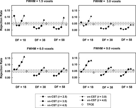
Results for the simulated stationary null fMRI data. Both methods were compared for three sample sizes (df = 18, 38 and 58) and three smoothness levels (FWHM =1.5, 3, 6 and 9 voxels). For vn‐CST, the applied CDT were 2.5 to 4.5. The desired FWE‐corrected P‐value of the test was 0.05.

Figure 2 shows the FWE‐corrected rejection rates on simulated non‐stationary null data. The rejection rates for TFCE for all six levels of non‐stationarity are 0.043 to 0.063, 0.035 to 0.041, and 0.044 to 0.06 for df = 18, 38 and 58, respectively. vn‐CST controls the rejection rates well when CDT < 4.0 under all levels of non‐stationarity. The performance of vn‐CST is somewhat liberal when CDT > 4.0, especially for low df (df = 18). These data suggest that TFCE shows more accurate and stable performance than vn‐CST under all chosen levels of non‐stationarity.

Figure 2.

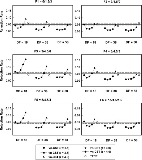
Results for the simulated non‐stationary null fMRI data. Six different non‐stationarity settings were used. All methods were compared for different sample sizes (df = 18, 38 and 58). For vn‐CST, the applied CDTs were 2.5 and 4.5. The desired FWE‐corrected P‐value of the test was 0.05.

Simulated activation data

Figure 3 shows the AUC results for the simulated stationary task activation data. The best performance for both methods were observed for FWHM = 1.5 voxels. In this case, vn‐CST shows higher sensitivity whe CDT = 3.5. With a suitable CDT, the performance of vn‐CST is comparable with that of TFCE, especially for higher SNR (SNR ≥ 3) and lower smoothness level (FWHM = 1.5 voxels).

Figure 3.

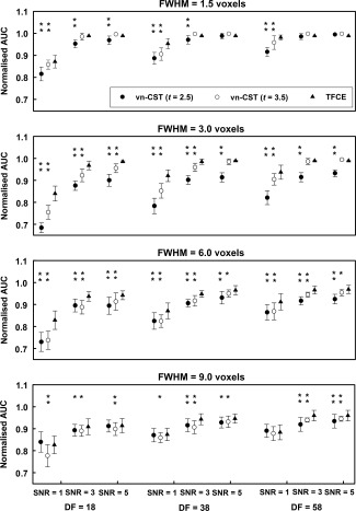
AUC results for the simulated stationary activation fMRI data. Both methods were compared for three sample sizes (df = 18, 38 and 58) and four smoothness levels (FWHM = 1.5, 3, 6 and 9 voxels). The applied SNRs were 1, 3 and 5. For vn‐CST, the results of CDTs of 2.5 and 3.5 were shown. The FWE‐corrected P‐value of the test was 0.05. All vn‐CST significance levels are compared with those using TFCE (*: P < 0.05, **: P < 0.001).

Figure 4 shows the AUC results on simulated non‐stationary activation data. TFCE shows better performance under all conditions. For the selected parameters, the sensitivity of vn‐CST is increased with increasing CDT. With a suitable CDT (e.g., CDT = 3.5), there is no significant difference between TFCE and vn‐CST methods for higher SNR (SNR ≥ 3) and higher dfs (df ≥ 38).

Figure 4.

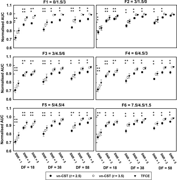
AUC results for the simulated non‐stationary task fMRI data. Six different non‐stationarity settings were used. All methods were compared for different sample sizes (df = 18, 38 and 58) and SNRs (SNR = 1, 3 and 5). For vn‐CST, the results for CDTs of 2.5 and 3.5 are shown. The FWE‐corrected P‐value of the test was 0.05. All vn‐CST significance levels are compared with those using TFCE (*: P < 0.05, **: P < 0.001).

Based on Figs. 3 and 4, the performances of both methods are increased with increasing df, especially for low SNR (SNR = 1). Based on the simulated null data analysis (e.g., that vn‐CST is a little lenient when CDT > 4.0), and limited space, we only show the results of CDT = 2.5 and 3.5 for vn‐CST method. For Figs. 3 and 4, the error bars representing the variability of the AUC under each condition (e.g., each df and SNR) are obtained from the 20 realizations generated for each sample size.

rfMRI‐Based Simulation Results

Figure 5 shows the TPR for the group‐level analysis at the significance level of 0.05. Figure 6 shows the corresponding activation map with CDT = 3.0 for vn‐CST method. Based on these results, both CST and TFCE methods show better performance when FWHM = 1.5 voxels. All the activation regions can be detected by TFCE and vn‐CST for high CDTs when FWHM = 1.5 voxels. With increasing FWHM of the applied Gaussian filter, the specificity and sensitivity decrease for both methods. Some smaller clusters are not detected by both methods when FWHM = 3.0 voxels. In our results, the sensitivity of vn‐CST increases with increasing CDT (corresponding to decreasing spatial extent). The performances of TFCE and vn‐CST methods were comparable when CDT ≥ 4.0 for vn‐CST.

Figure 5.

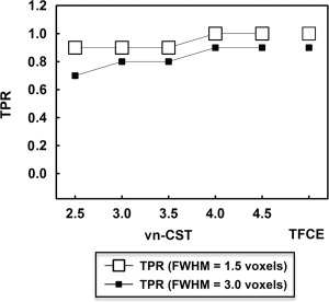
TPR for the group‐level rfMRI data analysis. The significance level was set to FWE‐corrected P = 0.05 and CDTs = 2.5, 3.0, 3.5, 4.0 and 4.5 are shown for vn‐CST. FWHMs of the applied Gaussian filters were 1.5 and 3 voxels. No false positive clusters were detected by vn‐CST or TFCE at either smoothness level.

Figure 6.

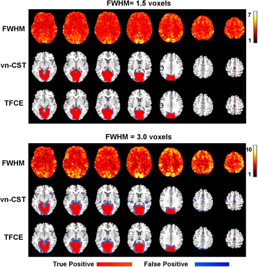
The detected activation map for the group‐level rfMRI analysis at the significance level of 0.05. For vn‐CST, the CDT was 3.0. FWHMs of the applied Gaussian filters were 1.5 voxels (top four rows) and 3 voxels (bottom four rows). Rows 1 and 4 show the variation in image smoothness using the voxelation‐corrected local smoothness based on Eq. (1) (obtained as RPV_ic^(1/3)). A region that was significant with TFCE but not vn‐CST was shown in black circles. [Color figure can be viewed at http://wileyonlinelibrary.com]

VBM Data Results

For the null VBM data analysis comparing the two groups of NC data (with no added signals), there were no regions with significant differences detected by TFCE or vn‐CST (for all CDTs) methods at FWE‐corrected P‐value < 0.05 (the results were not shown here). Figure 7 shows the TPR for the simulated inter‐group VBM analysis using vn‐CST and TFCE methods at the significance level of 0.05, for both levels of smoothness. Figure 8 shows the inter‐group VBM activation map with CDT = 3.0 for vn‐CST. No false positive clusters were detected by vn‐CST or TFCE at either smoothness level. TFCE detected all regions with simulated group differences for both smoothness levels, showing better sensitivity than vn‐CST. The sensitivity of vn‐CST is increased with increasing CDT and decreasing smoothness level, with all regions with simulated group differences being detected by vn‐CST when CDT = 4.5 and FWHM = 1.5 voxels. However, this may be due to vn‐CST being somewhat liberal at high CDT. Some smaller clusters were not detected by vn‐CST at relatively higher spatial smoothness. Table II shows the results of the false negative clusters by vn‐CST at different CDTs and smoothness levels. In general, vn‐CST detected almost all the activation regions under different spatial smoothness regions, even include some smaller clusters (cluster size = 30, 34 and 38 voxels). However, the cluster with cluster size is 50 voxels in the regions with quite large local smoothness (almost twice larger than other regions) was not detected when CDT < 4.5.

Figure 7.

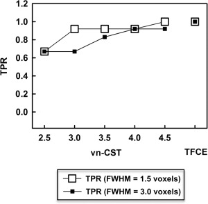
TPR for the simulated inter‐group differences VBM analysis using vn‐CST and TFCE methods at the significance level of 0.05. For vn‐CST, results are shown with CDTs = 2.5, 3.0, 3.5, 4.0 and 4.5. FWHMs of the applied Gaussian filters were 1.5 and 3 voxels. There were no detected false‐positives for either TFCE or vn‐CST.

Figure 8.

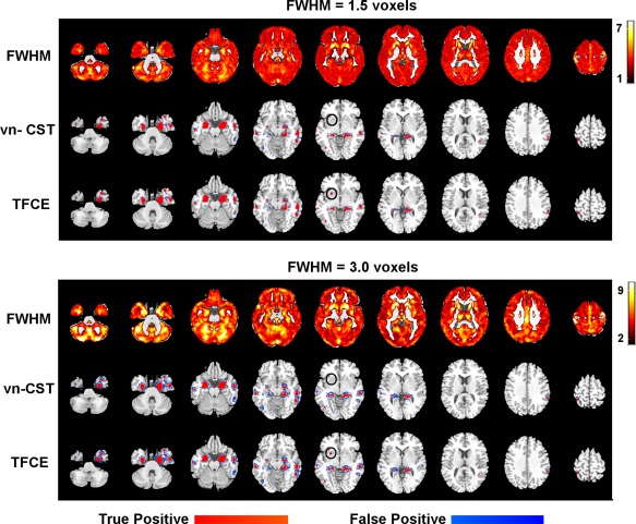
VBM results for the analysis with simulated inter‐group differences using vn‐CST and TFCE methods. FWE‐corrected P‐value was set to 0.05. For vn‐CST, the CDT = 3.0. FWHMs of the applied Gaussian filters were 1.5 voxels (top three rows) and 3 voxels (bottom three rows). Rows 1 and 4 show the variation in image smoothness using the voxelation‐corrected local smoothness based on Eq. (1) (obtained as RPV_ic^(1/3)). A region that was significant with TFCE but not vn‐CST was shown in black circles. [Color figure can be viewed at http://wileyonlinelibrary.com]

Table II.

VBM results of vn‐CST method

Cluster Size/voxels		2442	748	520	239	238	109	69	50	49	38	34	30
Applied FWHM= 1.5 voxels	Clusters' mean FWHM	4.64	5.66	4.12	3.93	3.53	3.29	3.41	8.82	3.66	4.02	4.20	3.25
	t‐value	2.5/3.0/3.5/4.0/4.5	2.5/3.0/3.5/4.0/4.5	2.5/3.0/3.5/4.0/4.5	2.5/3.0/3.5/4.0/4.5	2.5/3.0/3.5/4.0/4.5	2.5/3.0/3.5/4.0/4.5	2.5/3.0/3.5/4.0/4.5	4.5	3.0/3.5/4.0/4.5	3.0/3.5/4.0/4.5	2.5/3.0/3.5/4.0/4.5	3.0/3.5/4.0/4.5
Applied FWHM= 3.0 voxels	Clusters' mean FWHM	6.49	7.76	5.60	5.18	4.83	4.13	4.52	10.49	4.48	4.94	5.70	3.92
	t‐value	2.5/3.0/3.5/4.0/4.5	2.5/3.0/3.5/4.0/4.5	2.5/3.0/3.5/4.0/4.5	2.5/3.0/3.5/4.0/4.5	2.5/3.0/3.5/4.0/4.5	2.5/3.0/3.5/4.0/4.5	2.5/3.0/3.5/4.0/4.5		3.5/4.0/4.5	4.0/4.5	2.5/3.0/3.5/4.0/4.5	3.0/3.5/4.0/4.5

Cluster size is the voxel size of twelve known ground truth clusters.

Clusters' mean FWHM is the mean smoothness level (in voxels) of each cluster when FWHMs of the applied Gaussian kernel are 1.5 and 3.0 voxels, respectively. t‐value means all the CDTs that can detected each cluster when the applied FWHM are 1.5 and 3.0 voxels, respectively.

DISCUSSION

In this work we compared a new parametric statistical method, non‐stationary voxelation‐corrected cluster size tests (vn‐CST), with a widely used non‐parametric statistical method, TFCE, for group‐level analysis of both stationary and non‐stationary images under different dfs, SNRs, smoothness levels and CDTs (for CST methods).

Based on the results of the simulations using real rfMRI data, either vn‐CST or TFCE can be used for fMRI data analysis. Even though computer‐simulated data show that TFCE is clearly advantageous independent of CDTs and dfs and that the performance of vn‐CST in controlling false positive rates depends on the CDTs and is not as stable as TFCE, the simulations based on rfMRI data show comparable sensitivity and specificity of vn‐CST and TFCE for the most commonly used CDT (t‐value > 3) and degree of smoothing (1.5 voxels). The discrepancy between the rfMRI simulations and the computer‐simulations is likely due to computer‐simulated data not accurately simulating fMRI data. The simulation data based on rfMRI are much better at capturing the real properties of fMRI data, which was also asserted in the recent work by Eklund et al. [2016] that tested CSTs implemented in FSL and SPM. For VBM analyses, our findings show that while vn‐CST and TFCE do not identify any false positives, the true positive rate for vn‐CST varies with CDT and is only similar in performance to TFCE for the highest CDT (t‐value > 4). Thus, even though both TFCE and vn‐CST methods are applicable for non‐stationary data analysis, for VBM data, TFCE shows superior performance to vn‐CST, which does not completely eliminate the effect of spatial heterogeneity.

In this study, we found that vn‐CST can effectively control the false positives under both CDTs of P = 0.01 and 0.001. This represents a great advantage of vn‐CST over standard CST methods. Eklund et al. [2016] found that a CDT of P = 0.01 for the standard CST method (currently implemented in FSL and SPM) will yield a very high degree of false positives. Our modifications of the standard CST based on GRF to be applicable for non‐stationary data and low CDT makes this approach valid at typical CDT [Li et al., 2015]. Based on our simulation, the suggested CDTs for vn‐CST are between 2.5 and 4.0.

Based on all the simulated activation studies, it was found that both methods show better performance when the FWHM of the applied Gaussian kernel = 1.5 voxels. With increasing spatial smoothness, TFCE shows better performance than vn‐CST at detecting low SNR and small activation regions. This may be due to the increase in SNR produced by the TFCE output image in which the voxel‐wise values represent the amount of cluster‐like local spatial support. However, for real fMRI data in which the activation regions may be larger than the smaller activation regions we used in our simulations, the performance of vn‐CST and TFCE will be comparable (with a suitable CDT for vn‐CST).

We also found that the sensitivities of TFCE and vn‐CST methods are significantly increased with the increasing dfs, especially for low SNR (SNR = 1). In essence, a t‐statistic is a change divided by the square root of the estimated variance of that change. Analyses with fewer than about 20 dfs tend to have poor variance estimates. Errors in estimation of the variance appear as high (spatial) frequency noise in images, which cause noisy t‐statistics. This situation can be addressed by smoothing the variance images, replacing the variance estimate at each voxel with a weighted average of its neighbors [Nichols and Holmes, 2002].

There are several advantages of vn‐CST. It is suitable for both group‐level and single‐subject analysis and can preserve the high resolution of the single‐subject data by not requiring heavy spatial smoothing, and it addresses the failure of current widely used CSTs to control FWE and the limitations of TFCE with permutation testing for single‐subject analyses. In addition, vn‐CST is less computationally intensive than TFCE, which may be a negligible effect for most fMRI data analyses, but could be a limitation for studies with a large number of subjects and in other situations. For example, for the single group Monte Carlo simulations, CSTs ran in almost 10 seconds, whereas TFCE took almost 20 minutes with 1,000 permutations (1,000 permutations was chosen to achieve a reasonable time) (CPU 2.0 GHz, RAM 2GB).

CONCLUSIONS

In contrast to standard CSTs currently implemented in FSL, SPM, and the non‐parametric SPM toolbox, vn‐CST provides control over FWE at low CDT corresponding to P = 0.01. Overall, both TFCE and vn‐CST are nearly equally effective for group‐level analysis of fMRI data for CDT > 2.5. However, TFCE is more reliable and effective for group‐level analysis of VBM data without the requirement of high spatial smoothness and uniform spatial smoothness. The most suitable approach for inference may ultimately depend on whether or not the interest is in single‐subject versus group‐level analysis or on limitations associated with the greater computational demands of the TFCE approach.

Supporting information

Supporting Information

Supporting Information

Supporting Information

Supporting Information

Supporting Information

Supporting Information

Supporting Information

Supporting Information

Supporting Information

REFERENCES

- Benjamini Y, Heller R (2007): False discovery rates for spatial signals. J Am Stat Assoc 102:1272–1281. [Google Scholar]
- Cao J, Worsley KJ (2001): Applications of random fields in human brain mapping In: Moore M, editor. Spatial Statistics: Methodological Aspects and Applications, Vol. 159 Springer Lect Notes Stat. pp 169–182. [Google Scholar]
- Chumbley JR, Friston KJ (2009): False discovery rate revisited: FDR and topological inference using Gaussian random fields. Neuroimage 44:62–70. [DOI] [PubMed] [Google Scholar]
- Chumbley JR, Worsley KJ, Friston KJ (2009): Topological FDR for neuroimaging. NeuroImage 49:3057–3064. [DOI] [PMC free article] [PubMed] [Google Scholar]
- Douaud G, Smith S, Jenkinson M, Behrens TE, Johansen‐Berg H, Vickers J, James S, Voets N, Watkins K, Matthews P, James A (2007): Anatomically related grey and white matter abnormalities in adolescent‐onset schizophrenia. Brain 130:2375–2386. [DOI] [PubMed] [Google Scholar]
- Eklund A, Nichols TE, Knutsson H (2016): Cluster failure: Why fMRI inferences for spatial extent have inflated false‐positive rates. Proc Natl Acad Sci USA 113:7900–7905. [DOI] [PMC free article] [PubMed] [Google Scholar]
- Genovese CR, Lazar NA, Nichols T (2002): Thresholding of statistical maps in functional neuroimaging using the false discovery rate. NeuroImage 15:870–878. [DOI] [PubMed] [Google Scholar]
- Li H, Nickerson LD, Xiong J, Zou Q, Fan Y, Ma Y, Shi T, Ge J, Gao J‐H (2014): A high performance 3D cluster‐based test of unsmoothed fMRI data. NeuroImage 98:537–546. [DOI] [PubMed] [Google Scholar]
- Li H, Nickerson LD, Zhao X, Nichols TE, Gao J‐H (2015): A voxelation‐corrected non‐stationary 3D cluster‐size test based on random field theory. NeuroImage 118:676–682. [DOI] [PubMed] [Google Scholar]
- Forman SD, Cohen JD, Fitzgerald M, Eddy WF, Mintun MA, Noll DC (1995): Improved assessment of significant activation in functional Magnetic Resonance Imaging (fMRI): Use of a cluster‐size threshold. Magn Reson Med 33:636–647. [DOI] [PubMed] [Google Scholar]
- Friston KJ, Worsley KJ, Frackowiak RSJ, Mazziotta JC, Evans AC (1994): Assessing the significance of focal activations using their spatial extent. Hum Brain Mapp 1:210–220. [DOI] [PubMed] [Google Scholar]
- Glasser MF, Sotiropoulos SN, Wilson JA, Coalson TS, Fischl B, Andersson JL, Xu J, Jbabdi S, Webster M, Polimeni JR, Van Essen DC, Jenkinson M (2013): The minimal preprocessing pipelines for the Human Connectome Project. NeuroImage 80:105–124. [DOI] [PMC free article] [PubMed] [Google Scholar]
- Hayasaka S, Nichols TE (2003): Validating cluster size inference: Random field and permutation methods. NeuroImage 20:2343–2356. [DOI] [PubMed] [Google Scholar]
- Hayasaka S, Phan KL, Liberzon I, Worsley KJ, Nichols TE (2004): Nonstationary cluster‐size inference with random field and permutation methods. NeuroImage 22:676–687. [DOI] [PubMed] [Google Scholar]
- Holmes AP, Blair RC, Watson JDG, Ford I (1996): Nonparametric analysis of statistic images from functional mapping experiments. J Cereb Blood Flow Metab 16:7–22. [DOI] [PubMed] [Google Scholar]
- Kiebel SJ, Poline J‐B, Friston KJ, Holmes AP, Worsley KJ (1999): Robust smoothness estimation in statistical parametric maps using standardized residuals from the general linear model. NeuroImage 10:756–766. [DOI] [PubMed] [Google Scholar]
- Nichols TE, Holmes AP (2002): Nonparametric permutation tests for functional neuroimaging: A primer with examples. Hum Brain Mapp 15:1–25. [DOI] [PMC free article] [PubMed] [Google Scholar]
- Salimi‐Khorshidi G, Smith SM, Nichols TE (2011): Adjusting the effect of nonstationarity in cluster‐based and TFCE inference. NeuroImage 54:2006–2019. [DOI] [PubMed] [Google Scholar]
- Silver M, Montana G, Nichols TE (2011): False positives in neuroimaging genetics using voxel‐based morphometry data. NeuroImage 54:992–1000. [DOI] [PMC free article] [PubMed] [Google Scholar]
- Smith SM, Nichols TE (2009): Threshold‐free cluster enhancement: Addressing problems of smoothing, threshold dependence and localisation in cluster inference. NeuroImage 44:83–98. [DOI] [PubMed] [Google Scholar]
- Smith SM, Beckmann CF, Andersson J, Auerbach EJ, Bijsterbosch J, Douaud G, Duff E, Feinberg DA, Griffanti L, Harms MP, Kelly M, Laumann T, Miller KL, Moeller S, Petersen S, Power J, Salimi‐Khorshidi G, Snyder AZ, Vu AT, Woolrich MW, Xu J, Yacoub E, Uğurbil K, Van Essen DC, Glasser MF (2013): Resting‐state fMRI in the Human Connectome Project. NeuroImage 80:144–168. [DOI] [PMC free article] [PubMed] [Google Scholar]
- Worsley KJ (2002): Non‐stationary FWHM and its effect on statistical inference of fMRI data. Proceedings of the 8th International Conference on Functional Mapping of the Human Brain, June 2‐6, 2002, Sendai, Japan. NeuroImage 16 (2): Supplement 1:779–780.
- Worsley KJ, Marrett S, Neelin P, Vandal AC, Friston KJ, Evans AC (1996): A unified statistical approach for determining significant signals in images of cerebral activation. Hum Brain Mapp 4:58–73. [DOI] [PubMed] [Google Scholar]
- Worsley KJ, Andermann M, Koulis T, MacDonald D, Evans AC (1999): Detecting changes in nonisotropic images. Hum Brain Mapp 8:98–101. [DOI] [PMC free article] [PubMed] [Google Scholar]
- Zhou C, Wang YM (2009): New blockwise permutation tests preserving exchangeability in functional neuroimaging. Conf Proc IEEE Eng Med Biol Soc pp:6977–6980. [DOI] [PubMed] [Google Scholar]
Associated Data
This section collects any data citations, data availability statements, or supplementary materials included in this article.
Supplementary Materials