Imperfect (de)convolution may introduce spurious psychophysiological interactions and how to avoid it

Abstract

Psychophysiological interaction (PPI) is a widely used regression‐based method to study connectivity changes in different experimental conditions. A PPI effect is generated by point‐by‐point multiplication of a psychological variable (experimental design) and a physiological variable (time series of a seed region). If the psychological variable is non‐centered with a constant component, the constant component will add a physiological variable to the PPI term. The physiological component would in theory be accounted for by the physiological main effect in the model. But due to imperfect deconvolution and convolution with hemodynamic response function, the physiological component in PPI may no longer be exactly the same as the physiological main effect. This issue was illustrated by analyzing two block‐designed fMRI datasets, one simple visual checkerboard task and a set of different tasks designed to activate different hemispheres. When PPI was calculated with deconvolution but without centering, significant results were usually observed between regions that are known to have baseline functional connectivity. These results could be suppressed by simply centering the psychological variable when calculating the PPI term or adding a deconvolve–reconvolved version of the physiological covariate. The PPI results with centering and with deconvolve–reconvolved physiological covariate are consistent with an explicit test for differences in coupling between conditions. It was, therefore, suggested that centering of the psychological variable or the addition of a deconvolve–reconvolved covariate is necessary for PPI analysis. Hum Brain Mapp 38:1723–1740, 2017. © 2017 Wiley Periodicals, Inc.

INTRODUCTION

Studying brain functional connectivity using functional MRI (fMRI) has enabled great progress in mapping brain networks and brain functions in resting‐state [Biswal et al., 1995, 2010; Fox et al., 2005; Greicius et al., 2003]. However, brain functional connectivity is thought to be dynamic [Bullmore and Sporns, 2012; Park and Friston, 2013], and theories in cognitive neuroscience usually hypothesized that information flow between brain regions varies depending on task contexts. Therefore, it is essential to study task modulated connectivity, using methods such as psychophysiological interaction (PPI) [Friston et al., 1997] and dynamic causal modeling (DCM) [Friston et al., 2003]. Unlike DCM that is fully hypothesis‐driven, PPI implements regression‐based models, which enables voxel‐wise statistics. Given that task modulated connectivity it is still largely unknown, PPI is particularly desirable in the current state of research. The PPI method has been validated using simulations [Kim and Horwitz, 2008; McLaren et al., 2012], and has been widely used to investigate context dependent brain connectivity in different task domains [e.g., Di et al., 2017].

Because the blood‐oxygen‐level dependent (BOLD) signals in fMRI are an indirect measure of neural activity, it is critical for the PPI method to properly handle the asynchrony between an experimental design and its hemodynamic responses. In the psychophysiological interaction (PPI) framework, both task activations (the psychological variable) and task independent fluctuations of a seed region (the physiological variable) are modeled. And most importantly, the PPI model includes an interaction term between the task design and the seed time series. In a simple case where there is only one psychological variable, the general linear model (GLM) for the time series of a given voxel y could be expressed as follows:

$$y={\beta }_0+{\beta }_1\cdot x_{Psych}+{\beta }_2\cdot x_{Physio}+{\beta }_3\cdot x_{PPI}+\epsilon$$ (1)

where x_Psych represents the psychological variable, x_Physio represents the seed time series for physiological variable, and x_PPI represents the psychophysiological interaction. To account for hemodynamic delays, early implementation of PPI calculated the psychological variable by convolving a box‐car psychological function with a hemodynamic response function (HRF) (Fig. 1). The PPI term is then calculated by point‐by‐point multiplication between the physiological variable x_Physio (Fig. 1A) and (mean centered) psychological variable x_Psych (Fig. 1E):

$$x_{PPI}=x_{Psych}\cdot x_{Physio}$$ (2)

Figure 1.

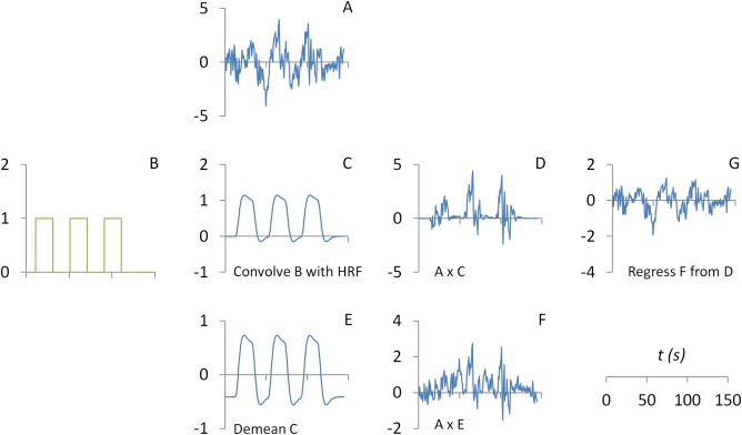
Illustrations of the calculation of psychophysiological interaction (PPI) without deconvolution. The part figure (A) shows the time series of a seed region. The part figure (B) shows a box‐car function representing task on (coded as 1) and off (coded as 0). The box‐car function is convolved with the canonical hemodynamic response function (HRF) to form a predicted psychological variable at the BOLD (blood‐oxygen‐level dependent) level (C). A PPI term (D) could then be calculated by point‐by‐point multiplication between the physiological variable (A) and psychological variable (C). A PPI term (F) could also be calculated by point‐by‐point multiplication between the physiological variable (A) and a demeaned version of psychological variable (E). Because the psychological variable (C) contains a constant component, the resulting PPI (D) contains a component of the physiological variable. It could be illustrated by removing the PPI with centering (F) from the PPI without centering (D), which results in a residual of G. The residual G and the physiological variable (A) are essentially the same. Green color represents variables at the neuronal level, and blue color represents variables at the BOLD level. [Color figure can be viewed at http://wileyonlinelibrary.com]

To better illustrate the meaning of the interaction term, we put Eq. (2) into Eq. (1), and rewrote it as:

$$\begin{array}{c}y={\beta }_0+{\beta }_1\cdot x_{Psych}+{\beta }_2\cdot x_{Physio}+{\beta }_3\cdot x_{Psych}\cdot x_{Physio}+\varepsilon \\ ={\beta }_0+{\beta }_1\cdot x_{Psych}+({\beta }_2+{\beta }_3\cdot x_{Psych})\cdot x_{Physio}+\varepsilon \end{array}$$ (3)

It shows that the relationship between the seed region x_Physio and target region y is expressed as β₂ + β₃ · x_Psych, which is a linear function of task design x_Psych. This task dependent regression coefficient can now be regarded as an estimate of effective connectivity that couples the seed region to the test or target region. Crucially, this connectivity changes in a context sensitive way with the psychological variable.

We note that it is in general advisable to center (subtract the mean from a variable) the two main effect variables before calculating the interaction term, because otherwise the correlations between the interaction term and main effects would be very high. In the case of PPI calculation, the PPI term (Fig. 1D) could be calculated by multiplication between the physiological variable (Fig. 1A) and the non‐centered psychological variable (Fig. 1C). We use $x_{\mathrm{Psych}}^{*}$ to represent the non‐centered psychological variable, and it could be expressed as $x_{\mathrm{Psych}}^{*}$ = x_Psych + c, where c represents a constant. The PPI term without centering the psychological variable $x_{\mathrm{PPI}}^{*}$ becomes:

$$\begin{array}{c}{x}_{PPI}^{*}=x_{Psych}^{*}\cdot x_{Physio}\\ =(x_{Psych}+c)\cdot x_{Physio}\\ =x_{Psych}\cdot x_{Physio}+c\cdot x_{Physio}\\ =x_{PPI}+c\cdot x_{Physio}\end{array}$$ (4)

Therefore, the PPI term without centering the psychological variable contains a component of the physiological main effect. This could be visually illustrated by regressing out x_PPI (Fig. 1F) from $x_{\mathrm{PPI}}^{*}$ (Fig. 1D). The residual (Fig. 1G) turns out to be almost identical to the physiological variable. The physiological component in the non‐centered PPI term may lead to high correlation between the PPI and physiological main effect. However, because the main effect of physiological variable is always added in the GLM as a covariate [Eq. (1)], the collinearity would not be a problem. Using PPI terms with or without centering would generate exactly the same PPI effects (see Appendix).

The above mentioned approach only works when the psychological variable changes slowly relative to the hemodynamic response. If the psychological variable changes quickly relative to the hemodynamic response time constants, it is generally advisable to deconvolve the hemodynamic response from observed time series before constructing the interaction term [Gitelman et al., 2003]. We use z to represent variables at the neuronal level, and * to represent convolution operator. The deconvolution process of the physiological variable x_Physio means to find a variable z_Physio, so that:

$$x_{Physio}=z_{Physio}\ast hrf$$ (5)

In SPM, hemodynamic deconvolution was performed using an empirical Bayes procedure [Friston et al., 2002; Gitelman et al., 2003]. Once the deconvolved physiological time series z_Physio (Fig. 2B) was calculated, the PPI term could then be calculated by multiplying z_Physio with a centered box‐car psychological function z_Psych (Fig. 2G), and then convolve it with HRF (Fig. 2H,I).

$$x_{PPI}=(z_{Psych}\cdot z_{Physio})\ast hrf$$ (6)

Figure 2.

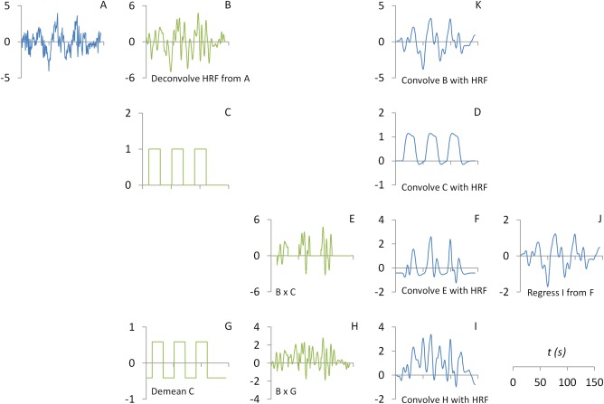
Illustrations of the calculation of psychophysiological interaction (PPI) with deconvolution. The part figure (A) shows the time series a seed region. The time series (A) is deconvoved with the canonical hemodynamic response function (HRF) to form a neuronal level physiological variable (B). The part figure (C) shows a box‐car function representing task on (coded as 1) and off (coded as 0), which is then convolved with a canonical HRF to form a psychological variable at the BOLD (blood‐oxygen‐level dependent) level (D). A PPI term (F) is calculated by first point‐by‐point multiplication between the physiological variable (B) and psychological variable (C) (as shown in E), and then convolved with the canonical HRF to form a PPI term at the BOLD level. A PPI term (I) could also be calculated using a centered psychological variable (G). Because the psychological variable (C) contains a constant component, the resulting PPI (F) contains a component of the physiological variable. It could be illustrated by removing the PPI with centering (I) from the PPI without centering (F), which results in a residual of J. Even though the residual J is still highly correlated with the physiological variable (A), they are not exactly the same. The discrepancy is caused by imperfect deconvolution and convolution processes with the HRF. If the physiological variable is deconvolved with the HRF (B), and convolved back with the HRF, the resulting variable (K) is exactly the same as the residual J. Green color represents variables at the neuronal level, and blue color represents variables at the BOLD level. [Color figure can be viewed at http://wileyonlinelibrary.com]

Again, if the psychological box‐car function $z_{\mathrm{Psych}}^{*}$ was not centered, the PPI term is then expressed as the following equation:

$$\begin{array}{c}{x}_{PPI}^{*}=(z_{Psych}^{*}\cdot z_{Physio})\ast hrf\\ =[(z_{Psych}+c)\cdot x_{Physio}]\\ =(z_{Psych}\cdot z_{Physio})\ast hrf+(c\cdot z_{Physio})\ast hrf\\ =x_{PPI}+c\cdot z_{Physio}\ast hrf\end{array}$$ (7)

Comparing with the PPI term with centering (Fig. 2I), the $x_{\mathrm{PPI}}^{*}$ (Fig. 2F) contains a component of physiological variable c·z_Physio*hrf. This physiological component can be visualized by regressing out x_PPI from $x_{\mathrm{PPI}}^{*}$ (Fig. 2J). Even though the general trend of the physiological component is quite similar to the original physiological variable (Fig. 2A), clear differences could be seen. The physiological component in PPI (Fig. 2J) is smoother than the original signal. We argue that it is because of imperfect deconvolution and convolution processes. We can also directly convolve the deconvolved physiological variable z_Physio with HRF. And it could be seen that the resulting time series (Fig. 2K) turns out to be identical to the physiological component (Fig. 2J). Because it is the original physiological variable (Fig. 2A) which will be added in a PPI GLM model, the original physiological variable could no longer fully account for the physiological component in a PPI term. This could result in spurious PPI effects that could not be accounted for by the main effects.

A real fMRI experiment usually has more than one experimental condition in addition to an implicit baseline. Theoretically, the total n conditions could be modeled using n – 1 psychological variables using many different ways. A straightforward way is to model each of the experimental condition with respect to all other conditions (with the implicit baseline not modeled) [McLaren et al., 2012]. In such a framework, the calculation of PPI term for each condition faces the same problem as has been described above.

The current study was motivated by our observations in our lab that some regions that are known to be highly correlated with the seed regions are likely to show positive PPI effects. In earlier version of SPM, it did not center the psychological variable when calculating the PPI term. Given that PPI calculated with deconvolution and without centering contains a physiological main effect component that could not be fully taken into account by the physiological main effect covariate, we predicted that spurious PPI results may take place in brain regions who has high baseline functional connectivity with the seed regions. The aim of the present study is firstly to demonstrate that with and without centering would generate different PPI results. To establish the construct validity of the different PPI approaches, we calculated correlation differences between conditions. We predict that centering when calculating PPI term will produce results that reflect differences in correlation (functional connectivity) in relation to the results with not centering. We also considered the addition of a deconvolve–reconvolved version of the physiological variable as a covariate to remove potential confounds. We present two block‐designed fMRI studies. The first is a simple flickering checkerboard task against a fixation condition. We adopted a typical PPI analysis protocol, that is, performing “conventional” GLM analysis to identify regions that were activated by the checkerboard stimulations, and performing PPI analysis using these regions to identify regions that had task modulated connectivity with them. In what follows, we analyzed fMRI data from six different tasks conditions. We defined 160 regions of interest (ROIs) sampling the whole brain [Dosenbach et al., 2010] to calculate pair wise PPI effects of the six task conditions against their respective fixation conditions.

MATERIALS AND METHODS

Visual Checkerboard Task

We first used a simple visual checkerboard task to illustrate the effects of mean centering on PPI effects. This is a simple block‐designed task, with an experiment condition of flickering checkerboard presentation versus a control condition of simple fixation. The analysis strategy followed commonly used strategy of PPI analysis; that is, first identifying regions that were activated in the task, and performing PPI analysis using these regions. Specifically, we expected that the conventional general linear model (GLM) could show reliable activations of the visual cortex in the checkerboard condition compared with fixation condition. Therefore, we used the activated visual regions as seeds to perform PPI analysis to show which regions in the brain that have task modulated connectivity with the visual seeds during the checkerboard condition compared with the fixation condition.

Subjects

The data were adopted from the Enhanced Nathan Kline Institute—Rockland Sample (http://fcon_1000.projects.nitrc.org/indi/enhanced/). We used a subset of data from the release 1, which the subjects were all adult subjects without any mental and physical diseases. The data were also discarded if a subject's head motion was greater than 3 mm or 3° during the experiments. As a result, data from 26 subjects (8 females) were included in the analysis. The mean age of the sample was 31.7 years (18–60 years).

Visual checkerboard tasks

The block designed fMRI experiment consisted of 20 s of fixation condition and 20 s of flickering checkerboard condition repeated three times. The remaining period until fMRI scan complete was blank screen. Only the data with a TR (repetition time) of 0.645 s were used. 239 or 240 of fMRI images were scanned in total for each subject.

MRI scan parameters

MRI data were scanned using a 3T Siemens Magnetom TrioTim syngo MR B17 scanner. The following parameters were used to scan the fMRI data: TR = 645 ms; TE = 30 ms; flip angle = 60°; voxel size = 3 mm³ isotropic; number of slices = 40. The following parameters were used to scan the MPRAGE (magnetization‐prepared rapid acquisition with gradient echo) T1 images: TR = 1900 ms; TE = 2.52 ms; flip angle = 9°; voxel size = 1 mm³ isotropic. More information of the data can be found in Nooner et al. [2012].

MRI imaging processing

Preprocessing

Imaging data preprocessing and analysis were performed using SPM8 (http://www.fil.ion.ucl.ac.uk/spm/) under MATLAB (http://www.mathworks.com/). The first 14 images (∼9 s) were discarded from analysis. The last image was also discarded if there were 240 images in total, so that the number of remaining images for each subject was 225. The functional images for each subject were then realigned to adjust displacements due to head motion, and coregistered to the subject's own high resolution T1 image. The T1 images were segmented and normalized into standard Montreal Neurological Institute (MNI) space using the new segment function in SPM8. The deformation field maps from the segmentation step were used to normalize functional images into MNI space. During normalization, the functional images were resampled at 3 × 3 × 3 mm³ spatial resolution. Finally, the functional images were spatially smoothed using an 8 mm full‐width at half maximum (FWHM) Gaussian kernel.

Activation analysis

A general linear model (GLM) was first built for each subject to detect regions that had higher activity in the checkerboard condition than in the fixation condition. A box‐car function convolved with canonical hemodynamic response function (HRF) was used to model task activations. In addition to the task predictor, 24 motion parameter time series were also added in the GLM to minimize the effects of head motion [Friston et al., 1996], as well as two regressors representing the first eigenvariate of white matter (WM) signals, and the first eigenvariate of cerebrospinal fluid (CSF) signals. The parameter estimates (β) maps for each subject representing activations by checkerboard stimulation were used for group‐level analysis of one sample t‐test. Not surprisingly, reliable activations could be observed in the visual cortex. Therefore, two regions from the left and right middle occipital gyrus (MOG) were selected, respectively, based on maxima activations in each hemisphere. The MNI coordinates of the two regions were −24, −91, 4 for the left MOG (LMOG), and 27, −94, 10 for the right MOG (RMOG).

PPI analysis

For each subject, spherical ROI were defined, centered at the peak coordinates of the LMOG and RMOG seeds, with a radius of 8 mm. The first eigenvariate was extracted after adjusting for head motion and WM/CSF signals. This time series was the physiological variable. The psychological variable was defined by a box‐car function convolved with the canonical HRF. The PPI terms were calculated in four different ways based on whether the physiological variable was deconvolved and whether the psychological variable was mean centered. We included the non‐deconvolved method to better illustrate our derivation in the introduction. And this method is still used in other fMRI software such as FSL (FMRIB Software Library) [Jenkinson et al., 2012]. The first PPI was calculated with deconvolution and with psychological variable not centered (Fig. 3 Model 1). Practically, a seed time series was deconvolved with the canonical HRF, so that the resulting time series represented activities at the neuronal level. Then the deconvolved seed time series was demeaned, and multiplied with the non‐demeaned psychological box‐car function. This was the default option in SPM after revision r3271 in SPM5 and before revision r6556 in SPM12. The second PPI was calculated with deconvolution and with psychological variable centered (Model 2). The deconvolved seed time series was demeaned, and multiplied with the demeaned psychological box‐car function. This was the default option in SPM12 after revision r6556. The third PPI was calculated without deconvolution and without psychological variable centered (Model 3). The psychological box‐car function was convolved with the canonical HRF and multiplied with the raw physiological time series. And the fourth PPI was calculated without deconvolution and with psychological variable centered (Model 4). The psychological box‐car function was convolved with the canonical HRF, centered, and then multiplied with the raw physiological time series. In addition to these three regressors, 24 variables for head motions, and 2 variables of WM and CSF signals, and a constant term were also included in the GLMs. Lastly, to illustrate that the significant effects using the Model 1 may be due to artifact of deconvolution and reconvolution, we added the deconvolve–reconvolved variable as a covariate to Model 1, which formed the Model 5. Separate analyses were conducted for the LMOG and RMOG seeds. The β maps representing the PPI effects were used for group level analysis. One sample t‐test was performed for each of the four PPI analyses, separately. The resulting statistical maps were first set as P < 0.001, and a cluster‐level correction of false discovery rate (FDR) of P < 0.05 was used to identify statistically significant clusters. To illustrate the spatial distributions of the deconvolve–reconvolve effects, the corresponding β maps in Model 5 were also analyzed in terms of group level one sample t‐test.

Figure 3.

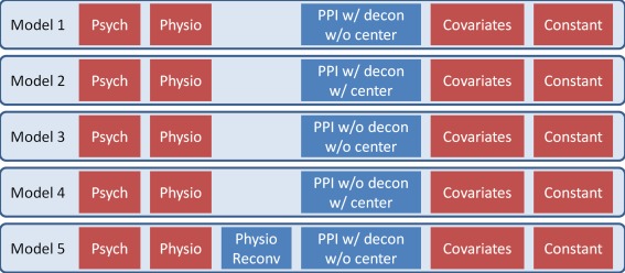
Illustrations of five general linear models (GLMs) for different psychophysiological interaction analysis. Red blocks represent the variables that are kept the same in all the five GLMs. They include a psychological variable of a (non‐centered) box‐car function convolved with hemodynamic response function (HRF), a physiological variable, covariates including white matter/cerebrospinal fluid signals and head motion models, and a constant term. The five models only differ in the blue blocks. [Color figure can be viewed at http://wileyonlinelibrary.com]

Direct comparisons of correlation differences

We expected different PPI results when the PPI terms were calculated in different ways. To establish which results reflect functional connectivity changes between task conditions, we directly calculated correlation differences of BOLD signals between the two experimental conditions. We defined two ROIs from the results of PPI analysis (see Results for details), and extracted their time series for each subject. The first six seconds of each block (either fixation or checkerboard) were discarded to get rid of transient hemodynamic responses (Fig. 4). The remaining time points of each block were first demeaned, and concatenated together for each condition. Pearson's correlation coefficients between the resulting ROIs and the seed regions were calculated for each condition and each subjects. The correlation coefficients were transformed into Fisher's z values, and compared between the checkerboard and fixation conditions using paired t‐test.

Figure 4.

Illustration of correlation difference calculation. Six seconds after onset of each (fixation or checkerboard) condition were removed from analysis to get rid of transient hemodynamic responses. Time points of different blocks of the same condition (indicated by red or blue) were demeaned for each block, and then concatenated together to calculate correlations. [Color figure can be viewed at http://wileyonlinelibrary.com]

Lateralization Tasks

Because the visual checkerboard task is a fairly simple task, the PPI analysis was restricted to visual seeds. We next analyzed an fMRI data of different tasks, which were designed to activate different regions and hemispheres of the brain [Cai et al., 2013]. Therefore, we focused on large scale brain connectivity between regions of the whole brain to evaluate how different tasks modulated large scale brain connectivity. In addition to these tasks, resting‐state fMRI data were also collected, so that we could study the relationships between task related connectivity changes and resting‐state connectivity strengths.

Subjects

Subjects were university students recruited from New Jersey Institute of Technology. All subjects were right handed, and had normal or corrected‐to‐normal vision. After removing subjects due to large head motion (>3 mm or 3°), 24 subjects were included in the current analysis (10 females). The mean age was 20.5 years old (18–25 years). Written consents were obtained from all the participants before MRI scanning. The study was approved by the institutional review board (IRB) at University of Medicine and Dentistry of New Jersey.

Task design

There were three tasks, each having an experimental condition and a control condition.

Landmark task

For each trial, a horizontal line appeared in the middle of the screen, which occupied the whole width of the screen. A small vertical line was also presented at the same time. In the experimental condition, the vertical line crossed the horizontal line in the middle. The vertical line was either in the center of the entire horizontal line, or slightly off the center to either left or right. The subjects were asked to judge whether the vertical line was on or off the center by pressing the left or right button of the response box. In the control condition, the vertical line was either intersecting with the horizontal line, or slightly up to the horizontal line without touching it. The subjects were asked to indicate whether the vertical line was intersecting or non‐intersecting the horizontal line with left or right button pressing of the response box.

Mental rotation task

The stimuli of the mental rotation experiment was obtained from Peters and Battista [2008]. For each trial, two pictures of the stimuli were presented side by side on the screen. The subjects needed to indicate whether the two pictures were the same stimuli or left/right mirrored. For the experimental condition, one of the pictures was rotated for some degree and mirrored or not mirrored. While for the control condition, the two pictures were either exactly the same or mirrored.

Word generation task

For the experiment condition, a letter was presented at the center of the screen. The subjects were asked to think about words started with the presented letter. For the control condition, four letters “baba” were presented. The subjects were asked to simply repeat reading “baba” silently, without thinking about specific words.

The three tasks were designed as three separate fMRI runs. All three experiments were block design. For each task run, the fMRI scan was started and ended with 20 s of fixation condition with a “+” presented at the center of the screen. Each task block lasted for 40 s, with 20 s fixation condition between each two task blocks. The experimental and control blocks were repeated four times. The order of experimental and control conditions were counterbalanced within a run. The total scan time for each task run was 8 min 20 s. The orders of the three tasks were counterbalanced across subjects. The subjects were familiarized with the three tasks before entering the MRI scanner.

In addition to the three tasks, a separate resting‐state run of 8 min was also collected. The subjects were asked to lay still and not think about anything particular. The resting‐state run was always scanned at the beginning of the MRI scan session to make sure that the “resting‐state” was not contaminated by other tasks.

MRI scan protocol

The MRI images were acquired at functional imaging center at New Jersey Medical School using a 3T Siemens Allegra scanner with a standard head only coil. With a TR of 2 s for all fMRI scans, we acquired 240 resting‐state fMRI images, and 250 fMRI images for each task run. The functional echo planar imaging (EPI) images were scanned using a gradient echo sequence with the following parameters: TR, 2 s; TE, 30ms; flip angle, 80°; slice thickness, 4 mm; in‐plane matrix size, 64 × 64; voxel size, 3.4375 × 3.4375 × 4 mm³; number of slices, 34. The co‐planar was aligned along the AC‐PC line, and the fMRI images covered the whole cerebral cortex and the superior portion of the cerebellum. Two dummy scans were automatically discarded at the beginning of each fMRI scan run.

In addition, high resolution T1 image for each subject was also collected at the end of the MRI scan session using MPRAGE sequence with the following parameters: TR, 2 s; TE, 4.38 ms; Flip angle, 8°; Slice Thickness, 1 mm; Matrix size, 256 × 256; voxel size, 0.859 × 0.859 × 1 mm³, FOV, 220 × 220.

Data processing and analysis

Preprocessing

Imaging data preprocessing and data analysis was also performed using SPM8. The preprocessing was in general the same, except that only two images of each fMRI run were discarded from analysis. Briefly speaking, all the functional images were realigned, and coregistered to subjects' own anatomical image. Subjects' data with head motion greater than 3 mm or 3° in any tasks were discarded. The anatomical image was segmented and normalized to standard MNI space. The deformation field maps were used to normalize all subjects' functional images into MNI space. The functional images were not smoothed because the subsequent analyses were all ROI based but not voxel based.

Activation analysis

Separate GLM models were built for the three tasks. For each task, the two task conditions were modeled as two box‐car functions convolved with the canonical HRF. Additionally, 24 regressors of Friston's head motion model [Friston et al., 1996], one regressor of the first eigenvariate of the WM signal, and one regressor of the first eigenvariate of the CSF signal were also added as covariates. Time series from 160 ROIs [Dosenbach et al., 2010] were extracted using the volume of interest function in SPM. During the time series extraction, effects of no interest were adjusted.

PPI analysis

We performed ROI based PPI analysis for the lateralization data, that is, the dependent variable was the time series of a ROI, instead of a voxel. Because the ROI time series were adjusted for head motion and WM/CSF signals, the PPI GLM model no longer included these regressors as covariates. In this analysis, we only focused on deconvolved methods, so that three PPI models were constructed for each pair of ROIs (Fig. 5). The PPI term was calculated separately for the two task conditions. In the first model, the PPI terms were calculated by point‐by‐point multiplication between non‐centered psychological box‐car function and deconvolved ROI time series, and then convolved with the canonical HRF. The GLM models included two regressors representing two task conditions, one regressor representing the time series of a ROI, and two regressors representing the PPIs for the two task conditions (Fig. 5A). In the second model, the PPI terms were calculated by point‐by‐point multiplication between centered psychological box‐car function and deconvolved ROI time series, and then convolved the canonical HRF. The main effects remained the same as those in Model 1 (Fig. 5B). Please notice the differences of the fourth and fifth regressors in Figure 5A,B. The third PPI model was the same as Model 1, except that a deconvolve–reconvolved version of the ROI time series (column 4 in Fig. 5C) was added as a covariate. The PPI GLMs were estimated between each pair of ROIs and for the three tasks. The corresponding β estimates of the PPI effects were used to form a 160 × 160 matrix representing task modulated connectivity of the task condition. The matrix of β ₄ of Model 3 was also calculated to illustrate the effect of deconvolution–reconvolution. The matrices were symmetrized by averaging corresponding lower and upper diagonal elements in the matrices (see Supporting Information). One sample t‐test was used to test whether a given effect was consistently different than 0 across subjects. FDR correction at P < 0.05 was used to correct for the total 12,720 (160 × 159/2) comparisons.

Figure 5.

Example design matrices for psychophysiological interaction (PPI) analysis of the lateralization tasks without centering (A), with centering (B), and without centering and with deconvolve–reconvolved physiological covariate (C). All the three methods are with deconvolution. The first two regressors represent two task conditions. The third regressor represents the time course of a seed region. The last regressor represents constant term. In A and B, the fourth and fifth regressors represent PPI effects of the two tasks, respectively. Please note the differences of the fourth and fifth regressors of the two matrices. C is the same as A except that an additional regressor (the fourth column) was added representing the deconvolve–reconvolved version of the physiological variable. Please note the differences between columns three and four in C.

Direct comparisons of correlation differences

For each task, we similarly grouped the time points into three conditions after removing the first three time points (6 s) at the beginning of each block; that is, the fixation condition, experimental condition, and control condition. The time points in each block were first mean centered, and concatenated in each condition. Pearson's correlation coefficients were calculated across the 160 ROIs for each condition. The correlation matrices were transformed into Fisher's z matrices. Then mean cross subject correlation Fisher's z matrices were subtracted between the task conditions and corresponding fixation conditions.

Resting‐state data

The time series of the 160 ROIs in resting‐state were extracted from the preprocessed fMRI data. When extracting the time series, 24 variables of head motion model, one variable of the first eigenvariate of the WM signal, and the first eigenvariate of the CSF signal were regressed out using a linear regression model. Temporal filtering was not performed to make sure that the connectivity measures were comparable between resting‐state and other task states. Spearman's correlation coefficients across 160 ROIs were calculated for each subject. The resulting correlations matrices were first transformed into Fisher's z scores, and averaged across subjects.

RESULTS

Visual Checkerboard Task

As expected, activations of the visual checkerboard task mainly involved bilateral posterior occipital regions, which were used for PPI analysis (the left penal in Fig. 6). PPI analysis of the LMOG and RMOG seeds only showed significant positive effects when using the deconvolved and non‐centered model (Model 1) but not all other four models (see Supporting Information Tables S1 and S2 for the lists of all significant clusters). The significant positive PPI effects were mainly located in the bilateral middle occipital gyrus. We show positive PPI effects of all the five models in Figure 6 using a threshold of P < 0.05 (uncorrected), not only to show significant effects in Model 1, but also to show non‐significant effects in models 2 through 5. The positive PPI effects in the bilateral middle occipital gyrus could only be observed in the deconvolved and non‐centered model (Model 1), but not when the psychological variable was centered (Model 2), or when not performing deconvolution. Please note that the results of non‐centered (Model 3) and centered (Model 4) effects without deconvolution were exactly the same, because the physiological main effect component in this case could be completely accounted for by the physiological main effect. Lastly, if we added a deconvolve–reconvolved physiological variable as a covariate to the Model 1 (i.e., Model 5), the positive PPI effects also disappeared. The spatial distributions of the deconvolution–reconvolution effects of the LMOG and RMOG are shown in Figure 7, with the bilateral middle occipital regions coincident with the positive PPI effects in Model 1. These further confirmed that the PPI effects in Model 1 might be artifact resulting from imperfect deconvolution–reconvolution processes on the physiological variable.

Figure 6.

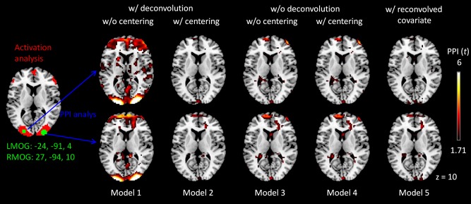
Positive psychophysiological interaction (PPI) effects of the left middle occipital gyrus (LMOG) (upper panels) and right middle occipital gyrus (RMOG) (lower panels) in the visual checkerboard task. The LMOG and RMOG seeds are illustrated in the left most column. The five remaining columns show PPI effects of five different models as illustrated in Figure 3. For illustration purpose, the PPI effect maps were thresholded at P < 0.05 (uncorrected). Z value and seeds coordinates are in MNI (Montreal neurological institute) space. [Color figure can be viewed at http://wileyonlinelibrary.com]

Figure 7.

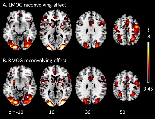
Effects of deconvolution–reconvolution of the seed signals of the left (A) and right (B) middle occipital gyrus (LMOG and RMOG). The effects represent the reconvolution regressor in model 5 in Figure 3. Clusters were thresholded at P < 0.001 uncorrected. Z values represent z coordinates in MNI (Montreal neurological institute) space. [Color figure can be viewed at http://wileyonlinelibrary.com]

In contrast, PPI analysis of the RMOG seed in all the PPI models but Model 1 showed significant negative PPI effects. The consistent clusters across the four models were located in the bilateral fusiform gyrus (BA 37) and supplementary motor area (SMA) (BA 32) (Fig. 8). We note that the analysis of LMOG seed showed a similar pattern of negative results, but the clusters did not survive a multiple comparison correction.

Figure 8.

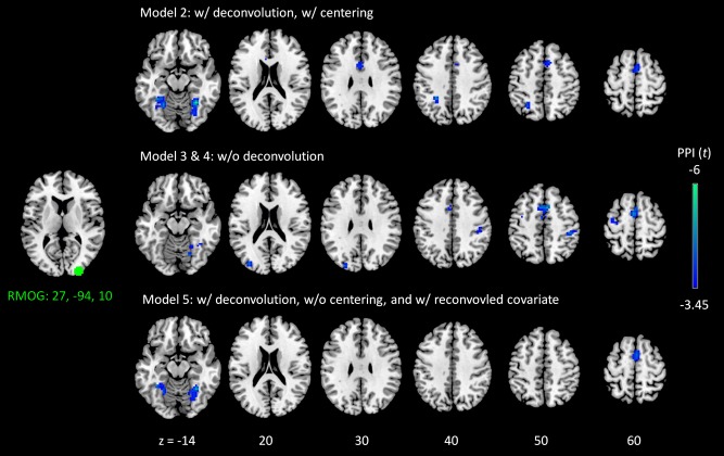
Negative psychophysiological interaction (PPI) effects of the right middle occipital gyrus (RMOG) in the visual checkerboard task. The RMOG seed is illustrated in the left most column. Model numbers correspond to the five PPI models in Figure 3. Please note that model 1 did not generate statistically significant results, and model 3 and 4 produced exactly the same results. The results were first thresholded at P < 0.001, and clusters were identified using cluster‐level false discover rate (FDR) at P < 0.05. Z values and seed coordinates are in MNI (Montreal neurological institute) space. [Color figure can be viewed at http://wileyonlinelibrary.com]

To get a sense which results were correct, we directly compared correlation differences between the two conditions. Correlation differences were calculated between the RMOG and LMOG, which showed positive PPI effects using the deconvolved and non‐centered method (Model 1). Correlation differences were also calculated between the RMOG and the three regions that showed consistent negative PPI effects when using other models (Model 2 through 5), that is, the left fusiform gyrus (LFuG) (centered at: −24, −55, −17), right fusiform gyrus (RFuG) (centered at: 30, −52, −14), and SMA (centered at: 9, 14, 49). As shown in Figure 9, the correlations (Fisher's z) between the LMOG and RMOG were not significantly different between the fixation condition (mean Fisher's z = 1.20) and checkerboard condition (mean Fisher's z = 1.09) (paired t test: t = 1.360, P = 0.186). In contrast, the correlations between the RMOG and FuG/SMA regions showed higher connectivity in the fixation condition than the checkerboard condition. Mean Fisher's z between RMOG and LFuG was 0.32 in the fixation condition and 0.14 in the checkerboard condition (paired t test: t = 3.063, P = 0.005). Mean Fisher's z between RMOG and RFuG was 0.38 in the fixation condition and 0.15 in the checkerboard condition (paired t test: t = 4.122, P < 0.001). Mean Fisher's z between RMOG and SMA was 0.17 in the fixation condition and −0.17 in the checkerboard condition (paired t test: t = 4.930, P < 0.001).

Figure 9.

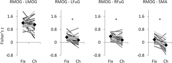
Correlations (Fisher's z) between ROIs (regions of interest) in the fixation (Fix) and checkerboard (Ch) conditions. Each line in the plots represents one subject. And the diamond markers represent means across subjects. LMOG, left middle occipital gyrus; RMOG, right middle occipital gyrus, LFuG, left fusiform gyrus; RFuG, right fusiform gyrus; Fix, fixation; Ch, checkerboard. * indicates statistical significant between the two conditions at P < 0.05.

Lateralization Tasks

Task activations of the six task conditions relative to their corresponding fixation conditions are shown in Supporting Information Figure S1. Typical activations in the visual cortex and distributed regions in the task positive networks, and negative activations in regions of the default mode network could be observed in all the six task conditions.

Task modulated connectivity across the 160 ROIs by the six tasks are illustrated in Figure 10. PPI effects without centering in general showed positive effects along the diagonal (Fig. 10A). Because the ROIs were sorted by their network affiliations defined by Dosenbach et al. [2010], the square like positive PPI effects reflected positive effects within each network. In contrast, PPI effects with centering showed generally smaller effects compared with PPI without centering, with many negative effects along the diagonal (Fig. 10B). Similar effects could be observed when adding deconvolve–reconvolved covariate (Fig. 10C). Interestingly, correlation differences calculated directly between task conditions (Fig. 10D) showed similar patterns to the PPI results with centering and with deconvolve–reconvolved covariate. The similarities among the matrices could be quantified by calculating correlations across elements in the lower diagonals of each matrix (Fig. 11). The correlations between PPI effects without centering and correlation differences were around 0.5 (0.47–0.55). In contrast, the PPI effects with centering and with deconvolve–reconvolved covariate generally showed larger correlations with correlation changes (all >0.7).

Figure 10.

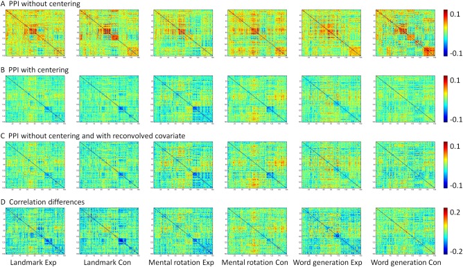
Matrices of task modulated connectivity across 160 ROIs estimated from PPI method without centering (A), with centering (B), without centering and with reconvolved covariate (C), and direct correlation differences (D). All PPI methods are with deconvolution. [Color figure can be viewed at http://wileyonlinelibrary.com]

Figure 11.

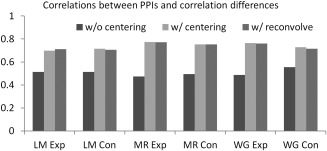
Correlations between task related connectivity changes estimated from PPI (without centering, with centering, and with reconvolved covariate) and correlation differences.

Figure 12 demonstrates significant task modulated connectivity for the six task conditions as revealed by PPI analysis with mean centering (see thresholded matrices in the Supporting Information). The majority of task modulated connectivity was negative, and mainly between regions within the visual network, and between regions within the sensorimotor network. There was a small number of increased connectivity, mainly between one region in the DMN and one region in the sensorimotor network or fronto‐parietal network.

Figure 12.

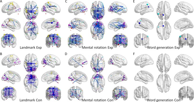
Increased (warm color) and decreased (cold color) functional connectivity for the six task conditions compared with their corresponding fixation conditions estimated from PPI analysis with centering. Statistical significant was determined using P < 0.05 after controlling multiple comparisons using false discovery rate (FDR). Data visualization used BrainNet Viewer [Xia et al., 2013]. [Color figure can be viewed at http://wileyonlinelibrary.com]

We next show the deconvolution–reconvolution effects for the three tasks in Figure 13. For reference, we also show resting‐state functional connectivity (correlation coefficients) calculated from a separate resting‐state session of the same group of subjects (Fig. 13D). It could be seen that the deconvolution–reconvolution effects highly resembled the resting‐state connectivity effects, that is, the higher a resting‐state connectivity between two ROIs the more likely one ROI showed correlations with deconvolve–reconvolved time series of the other ROI. These positive correlations caused positive correlations between PPI without centering and resting‐state connectivity strengths (Fig. 14). While, the pattern reversed when PPI were centered or the deconvolution–reconvolution covariate was added, that is, the task related connectivity generally showed small negative correlations with resting‐state strengths for five of the six task conditions, and task related connectivity of the word generation control condition showed close to zero correlation with resting‐state connectivity strengths.

Figure 13.

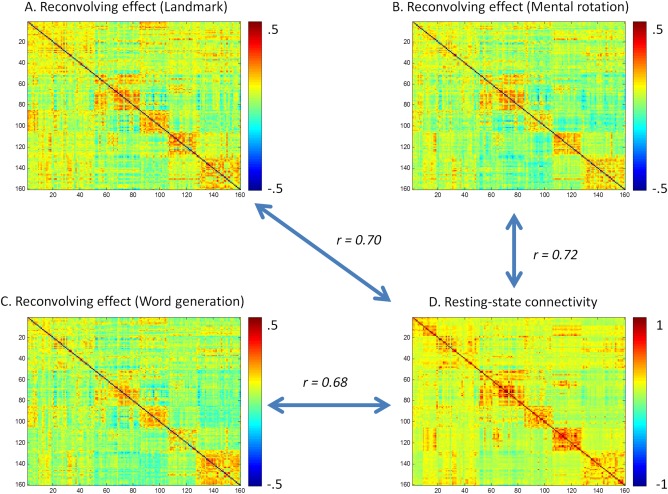
Deconvolution–reconvolution effects across the 160 ROIs for the three lateralization tasks (A through C), and the resting‐state functional connectivity matrix from a separate resting‐state run of the same subjects (D). [Color figure can be viewed at http://wileyonlinelibrary.com]

Figure 14.

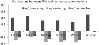
Correlations between resting‐state connectivity (mean Fisher's z scores) and PPI effects without centering, with centering, and with reconvolved physiological covariate.

DISCUSSION

We have presented a range of empirical results showing that not centering the psychological variable when calculating deconvolved PPI usually produce different results than using other PPI calculation methods. Adding a deconvolve–reconvolved physiological covariate could minimize the differences, and make the results more correlated with correlation differences between conditions.

For the checkerboard task, PPI without centering showed two main regions that had positive PPI effects with the LMOG and RMOG seeds; that is, the left and right middle occipital gyrus, which actually overlapped with the seeds themselves. These two regions were not only activated during the checkerboard task, but also showed high baseline correlations in resting‐state [Beckmann et al., 2005; Biswal et al., 2010; Lowe et al., 1998]. However, adding a deconvolve–reconvolved covariate of the physiological variable or centering the psychological variable when calculating PPI removed these PPI effects. In addition, the correlations between the LMOG and RMOG were not different between the checkerboard condition and fixation condition. Together, the positive PPI effects in the bilateral MOG are possibly artifactual derived from imperfect deconvolution–reconvolution processes. For the lateralization tasks, large PPI effects using deconvolved non‐centered method generally occurred between regions within a network, for example, the DMN, fronto‐parietal network, and the sensorimotor network. It is known that there are high baseline correlations between regions within the same network (e.g., Fig. 13CD). These square like within network effects were largely suppressed when performed centering, or included deconvolve–reconvolved covariate of the physiological variable. Taken together, the results also suggest that the significant PPI effects are artifacts produced by an imperfect deconvolution–reconvolution processes that cannot reproduce the original physiological regressor. This failure means that any physiological main effect in the PPI will not be explained away—and will appear as a significant effect that could be misinterpreted as an interaction.

For the checkerboard task, the regions that showed effects of deconvolve–reconvolved effects of the LMOG and RMOG resemble the regions that have high baseline correlations with two regions. Similarly for the lateralization tasks, the effects of deconvolve–reconvolved physiological covariate were also similar to the baseline connectivity between regions. Please note that the deconvolve–reconvolution physiological effects were obtained after taking into account the raw physiological effects. This is consistent with our prediction. The higher the baseline correlations between two regions, the higher the probability that the two regions have some nonlinear relationships that may give rise to high correlations with deconvolve–reconvolved effects. These additional correlations between a region's raw time series and another region's deconvolve–reconvolved effects may reflect some nonlinear effects between the two regions, which could not be explained by the raw physiological effects.

The PPI analyses with centering, without deconvolution, and with deconvolve–reconvolved covariate in general showed similar results, which are different from the results of PPI analysis with deconvolution but without centering. This inter‐method consistency also suggests the PPI results using centering, without deconvolution, or with deconvolve–reconvolved covariate represent meaningful task modulated connectivity. For the checkerboard task, we identified the bilateral fusiform gyrus (BA 37), and the SMA (BA 32) were consistently reported to have reduced connectivity with the right MOG seed in the checkerboard condition compared with the fixation condition. Further analysis validated these results, that is, the correlations between the MOG seeds and the three resultant regions had higher correlations in the fixation condition than in the checkerboard condition. Such reduced connectivity could also be directly illustrated by studying point‐by‐point dynamic connectivity changes using a sliding window method [Di et al., 2015]. The fusiform gyrus is part of the ventral visual pathway, and contained several regions involving processing different categories, for example, face [Kanwisher et al., 1997], human body [Peelen and Downing, 2005], and word form [Cohen et al., 2000]. Because the checkerboard stimulus is fairly simple, and cannot form a meaningful percept of a specific category, it is reasonable that the connectivity between the lower visual cortex and higher ventral visual areas such as fusiform gyrus decreased during the checkerboard stimulation. The SMA is part of the motor system. It may maintain certain amount of spontaneous connectivity with visual cortex. But since the checkerboard task did not require overt motor response, the spontaneous connectivity may be suppressed during the checkerboard presentation.

For the lateralization tasks, it was a little surprising to us that different task conditions in general showed decreased connectivity compared with corresponding fixation conditions. The decreased connectivity was generally observed between regions within the occipital network, and between regions within the sensorimotor network. However, similar patterns of more reduced connectivity in these networks have been observed previously [Cole et al., 2014], where the authors compared task related connectivity in task runs after removing task designs variables with connectivity in a separate resting‐state run. The current study demonstrated that, by using PPI, task related connectivity can be reliably studied by comparing different blocks within an fMRI run. Cole et al. [2014] also found many increased connectivity in tasks compared with resting‐state, mainly between regions from different networks. We could observe some similar positive effects in the PPI analysis with centering. However, the positive PPI effects could not reach significance, probably due the small sample size of the current study (n = 24) compared with Cole et al. (n = 118). All the experiment conditions of the lateralization tasks had visual stimulus presented, and the landmark task and mental rotation task also required overt manual response. Even so, the connectivity within the visual network and sensorimotor network still decreased. It is in line with a recent study showing that during visuospatial attention connectivity within the visual network decreased and connectivity between the visual region and regions in the attention networks increased [Spadone et al., 2015]. It may reflect a rebalance of within network and between network connectivity to ensure an efficient communications at the whole brain level.

Deconvolution was first introduced by Gitelman et al. [2003] to deal with hemodynamic delays in PPI analysis. It is a necessary step especially when a task block is short and in an extreme case, an impulse (i.e., event‐related design). The current results do not mean one should avoid decovolution when calculating PPI. However, caution is needed, because deconvolution is not a perfect process (because deconvolution in this context is an ill posed problem). On the other hand, the benefit of deconvolution on slow task designs (long block blocked design) has not yet been systematically examined. The current study showed that the PPI effects with centering and deconvolution on the checkerboard data are similar to those using non‐deconvolution PPI. Similarly, our previous study of physio‐physiological interactions also showed that with and without deconvolution generated similar results [Di and Biswal, 2013]. Studies are still needed to demonstrate the benefit of deconvolution for PPI analysis.

The current analysis suggests that simply centering the psychological variable before calculating PPI precludes spurious artifacts. Therefore, centering should always be performed. For an experiment with multiple conditions, it might be less problematic when directly comparing PPI effects between different experiment conditions, because the deconvolve–reconvolve artifact may be similar in the two conditions, thus being canceled out. However, it may be not the case if the physiological component has different weights for two task conditions, for example, the two task conditions have different numbers of blocks or trials. And practically, many studies reported PPI effects of an experimental condition compared with a baseline condition but not the well‐designed control condition. Performing centering would also prevent artifact when reporting PPI effects in this situation. An alternative way to prevent convolution artifact is to include a deconvolve–reconvolved version of the physiological variable as a covariate. It may be useful when the psychological variable was defined by complex contrast or higher‐order interactions (e.g., psycho‐physio‐physiological interaction, PPPI [Stamatakis et al., 2005]), where constant components may be not easy to remove.

A common argument against centering the psychological variable is interpretability. A coding of 1 for one condition, and 0 for other conditions seems to reflect connectivity only in the “1” condition but “zeroing out” other conditions. However mathematically, in either the non‐deconvolved case or the neurological timing case, the effect of removing the mean of psychological variable should only be a change in the resulting β weight of physiological variable and the overall mean β weight, as is shown in Eq. (A5). The reason for an effect on the PPI β is that x_physio from Eq. (A5) does not survive the deconvolution and reconvolution process. In addition, PPI is not designed to examine the connectivity in one condition, but the differences of connectivity between conditions. The PPI terms before and after centering are mathematically the same. Practically, because well‐structured functional connectivity is present without any explicit tasks, that is, in resting‐state [Biswal et al., 1995, 2010; Cordes et al., 2000], the goal of studying task‐related connectivity is never to study connectivity only in one task condition but the relative connectivity changes in one task compared with others. In short, centering the psychological variable does not affect the interpretability of PPI effects, and indeed makes the interpretation of the effects more straightforward.

We note that mean centering of the psychological variable was performed in earlier PPI articles [Friston et al., 1997; Gitelman et al., 2003]. It was the default setting in SPM2, and was removed in revision r3271 in SPM5. It becomes the default setting again in revision r6556 in SPM12. We recommend performing PPI analysis using the latest version of SPM, and the version information of SPM needs to be reported when reporting PPI results. AFNI (Analysis of Functional NeuroImages) [Cox, 1996] adopts a similar approach as SPM (https://afni.nimh.nih.gov/pub/dist/edu/data/CD.expanded/AFNI_data6/FT_analysis/PPI/README.txt). It does have an option to center the psychological variable. However, because the deconvolution process in AFNI is almost invertible with reconvolution, the reconvolved physiological variable is almost identical to the original one. So the effect of removing the mean in AFNI is very small. In addition, AFNI suggests removing psychological effects from the physiological variable before calculating PPI, which is an effective step to minimize collinearity between the PPI term and main effects. Lastly, FSL does not perform deconvolution when calculating the PPI term. Therefore, whether centering or not would not affect PPI results.

CONCLUSION

The present study demonstrated that not centering the psychological variable when calculating deconvolved PPI may result in spurious PPI effects. Simply centering the psychological variable could effectively suppress the artifacts. We also introduced to add a deconvolve–reconvolved physiological variable to suppress the artifacts, which may be useful in complex circumstances.

Supporting information

Supporting Information

Centering The Psychological Variable Does Not Change The Interaction Effect (Without Deconvolution)

Given a seed region x_Physio, a tested region y, and a centered psychological variable x_Psych, the following PPI model can be used to estimate a set of effects [β¹₀, β¹₁, β¹₂, β¹₃]:

$$y={\beta }_0^1+{\beta }_1^1\cdot x_{Psych}+{\beta }_2^1\cdot x_{Physio}+{\beta }_3^1\cdot x_{Psych}\cdot x_{Physio}+\varepsilon$$ (A1)

Superscript 1 denotes the first set of effect estimates.

We now have a non‐centered psychological effect $x_{\mathrm{Psych}}^{*}$, which can be expressed as the centered psychological variable plus a constant value c.

$$x_{Psych}^{*}=x_{Psych}+c$$ (A2)

We can estimate a new PPI model with the non‐centered psychological variable $x_{\mathrm{Psych}}^{*}$:

$$y={\beta }_0^2+{\beta }_1^2\cdot x_{Psych}^{*}+{\beta }_2^2\cdot x_{Physio}+{\beta }_3^2\cdot x_{Psych}^{*}\cdot x_{Physio}+\varepsilon$$ (A3)

This model gives a new set of effects [β²₀, β²₁, β²₂, β²₃]. Put Eq. (A2) into Eq. (A3):

$$y={\beta }_0^2+{\beta }_1^2\cdot (x_{Psych}+c)+{\beta }_2^2\cdot x_{Physio}+{\beta }_3^2\cdot (x_{Psych}+c)\cdot x_{Physio}+\varepsilon$$ (A4)

And match terms in Eq. (A4) with Eq. (A1):

$$y=\left({\beta }_0^2+{\beta }_1^2\cdot c\right)+{\beta }_1^2\cdot x_{Psych}+\left({\beta }_2^2+{\beta }_3^2\cdot c\right)\cdot x_{Physio}+{\beta }_3^2\cdot x_{Psych}\cdot x_{Physio}+\varepsilon$$ (A5)

Comparing Eq. (A5) with Eq. (A1), it can be seen that:

$$\begin{array}{c}{\beta }_0^1={\beta }_0^2+{\beta }_1^2\cdot c\\ {\beta }_1^1={\beta }_1^2\\ {\beta }_2^1={\beta }_2^2+{\beta }_3^2\cdot c\\ {\beta }_3^1={\beta }_3^2\end{array}$$

The effects of PPI with centering (β¹₃) and without centering (β²₃) remain the same. However, the parameter estimates of the physiological variable and constant term changed.

REFERENCES

- Beckmann CF, DeLuca M, Devlin JT, Smith SM (2005): Investigations into resting‐state connectivity using independent component analysis. Philos Trans R Soc Lond B Biol Sci 360:1001–1013. [DOI] [PMC free article] [PubMed] [Google Scholar]
- Biswal B, Yetkin FZ, Haughton VM, Hyde JS (1995): Functional connectivity in the motor cortex of resting human brain using echo‐planar MRI. Magn Reson Med 34:537–541. [DOI] [PubMed] [Google Scholar]
- Biswal BB, Mennes M, Zuo XN, Gohel S, Kelly C, Smith SM, Beckmann CF, Adelstein JS, Buckner RL, Colcombe S, Dogonowski AM, Ernst M, Fair D, Hampson M, Hoptman MJ, Hyde JS, Kiviniemi VJ, Kötter R, Li SJ, Lin CP, Lowe MJ, Mackay C, Madden DJ, Madsen KH, Margulies DS, Mayberg HS, McMahon K, Monk CS, Mostofsky SH, Nagel BJ, Pekar JJ, Peltier SJ, Petersen SE, Riedl V, Rombouts SARB, Rypma B, Schlaggar BL, Schmidt S, Seidler RD, Siegle GJ, Sorg C, Teng GJ, Veijola J, Villringer A, Walter M, Wang L, Weng XC, Whitfield‐Gabrieli S, Williamson P, Windischberger C, Zang YF, Zhang HY, Castellanos FX, Milham MP (2010): Toward discovery science of human brain function. Proc Natl Acad Sci U S A 107:4734–4739. [DOI] [PMC free article] [PubMed] [Google Scholar]
- Bullmore E, Sporns O (2012): The economy of brain network organization. Nat Rev Neurosci 13:336–349. [DOI] [PubMed] [Google Scholar]
- Cai Q, Van der Haegen L, Brysbaert M (2013): Complementary hemispheric specialization for language production and visuospatial attention. Proc Natl Acad Sci U S A 110:E322–E330. [DOI] [PMC free article] [PubMed] [Google Scholar]
- Cohen L, Dehaene S, Naccache L, Lehéricy S, Dehaene‐Lambertz G, Hénaff MA, Michel F (2000): The visual word form area: Spatial and temporal characterization of an initial stage of reading in normal subjects and posterior split‐brain patients. Brain 123 (Pt 2):291–307. doi: 10.1093/brain/123.2.291 [DOI] [PubMed] [Google Scholar]
- Cole MW, Bassett DS, Power JD, Braver TS, Petersen SE (2014): Intrinsic and task‐evoked network architectures of the human brain. Neuron 83:238–251. [DOI] [PMC free article] [PubMed] [Google Scholar]
- Cordes D, Haughton VM, Arfanakis K, Wendt GJ, Turski PA, Moritz CH, Quigley MA, Meyerand ME (2000): Mapping functionally related regions of brain with functional connectivity MR imaging. AJNR Am J Neuroradiol 21:1636–1644. [PMC free article] [PubMed] [Google Scholar]
- Cox RW (1996): AFNI: Software for analysis and visualization of functional magnetic resonance neuroimages. Comput Biomed Res 29:162–173. [DOI] [PubMed] [Google Scholar]
- Di X, Biswal BB (2013): Modulatory interactions of resting‐state brain functional connectivity. PLoS One 8:e71163. [DOI] [PMC free article] [PubMed] [Google Scholar]
- Di X, Fu Z, Chan SC, Hung YS, Biswal BB, Zhang Z (2015): Task‐related functional connectivity dynamics in a block‐designed visual experiment. Front Hum Neurosci 9:1–11. [DOI] [PMC free article] [PubMed] [Google Scholar]
- Di X, Huang J, Biswal BB (2017): Task modulated brain connectivity of the amygdala: A meta‐analysis of psychophysiological interactions. Brain Struct Funct 222:619–634. [DOI] [PMC free article] [PubMed] [Google Scholar]
- Dosenbach NUF, Nardos B, Cohen AL, Fair DA, Power JD, Church JA, Nelson SM, Wig GS, Vogel AC, Lessov‐Schlaggar CN, Barnes KA, Dubis JW, Feczko E, Coalson RS, Pruett JR, Barch DM, Petersen SE, Schlaggar BL (2010): Prediction of individual brain maturity using fMRI. Science 329:1358–1361. [DOI] [PMC free article] [PubMed] [Google Scholar]
- Fox MD, Snyder AZ, Vincent JL, Corbetta M, Van Essen DC, Raichle ME (2005): The human brain is intrinsically organized into dynamic, anticorrelated functional networks. Proc Natl Acad Sci U S A 102:9673–9678. [DOI] [PMC free article] [PubMed] [Google Scholar]
- Friston KJ, Williams S, Howard R, Frackowiak RS, Turner R (1996): Movement‐related effects in fMRI time‐series. Magn Reson Med 35:346–355. [DOI] [PubMed] [Google Scholar]
- Friston KJ, Buechel C, Fink GR, Morris J, Rolls E, Dolan RJ (1997): Psychophysiological and modulatory interactions in neuroimaging. Neuroimage 6:218–229. [DOI] [PubMed] [Google Scholar]
- Friston KJ, Penny W, Phillips C, Kiebel S, Hinton G, Ashburner J (2002): Classical and bayesian inference in neuroimaging: Theory. Neuroimage 16:465–483. [DOI] [PubMed] [Google Scholar]
- Friston KJ, Harrison L, Penny W (2003): Dynamic causal modelling. Neuroimage 19:1273–1302. [DOI] [PubMed] [Google Scholar]
- Gitelman DR, Penny WD, Ashburner J, Friston KJ (2003): Modeling regional and psychophysiologic interactions in fMRI: The importance of hemodynamic deconvolution. Neuroimage 19:200–207. [DOI] [PubMed] [Google Scholar]
- Greicius MD, Krasnow B, Reiss AL, Menon V (2003): Functional connectivity in the resting brain: A network analysis of the default mode hypothesis. Proc Natl Acad Sci U S A 100:253–258. [DOI] [PMC free article] [PubMed] [Google Scholar]
- Jenkinson M, Beckmann CF, Behrens TEJ, Woolrich MW, Smith SM (2012): FSL. Neuroimage. 62:782–790. [DOI] [PubMed] [Google Scholar]
- Kanwisher N, McDermott J, Chun MM (1997): The fusiform face area: A module in human extrastriate cortex specialized for face perception. J Neurosci 17:4302–4311. [DOI] [PMC free article] [PubMed] [Google Scholar]
- Kim J, Horwitz B (2008): Investigating the neural basis for fMRI‐based functional connectivity in a blocked design: Application to interregional correlations and psycho‐physiological interactions. Magn Reson Imaging 26:583–593. [DOI] [PubMed] [Google Scholar]
- Lowe MJ, Mock BJ, Sorenson JA (1998): Functional connectivity in single and multislice echoplanar imaging using resting‐state fluctuations. Neuroimage 7:119–132. [DOI] [PubMed] [Google Scholar]
- McLaren DG, Ries ML, Xu G, Johnson SC (2012): A generalized form of context‐dependent psychophysiological interactions (gPPI): A comparison to standard approaches. Neuroimage 61:1277–1286. [DOI] [PMC free article] [PubMed] [Google Scholar]
- Nooner KB, Colcombe SJ, Tobe RH, Mennes M, Benedict MM, Moreno AL, Panek LJ, Brown S, Zavitz ST, Li Q, Sikka S, Gutman D, Bangaru S, Schlachter RT, Kamiel SM, Anwar AR, Hinz CM, Kaplan MS, Rachlin AB, Adelsberg S, Cheung B, Khanuja R, Yan C, Craddock CC, Calhoun V, Courtney W, King M, Wood D, Cox CL, Kelly AMC, Di Martino A, Petkova E, Reiss PT, Duan N, Thomsen D, Biswal B, Coffey B, Hoptman MJ, Javitt DC, Pomara N, Sidtis JJ, Koplewicz HS, Castellanos FX, Leventhal BL, Milham MP (2012): The NKI‐rockland sample: A model for accelerating the pace of discovery science in psychiatry. Front Neurosci 6:152. [DOI] [PMC free article] [PubMed] [Google Scholar]
- Park HJ, Friston K (2013): Structural and functional brain networks: From connections to cognition. Science (80‐.) 342:1238411. [DOI] [PubMed] [Google Scholar]
- Peelen MV, Downing PE (2005): Selectivity for the human body in the fusiform gyrus. J. Neurophysiol 93:603–608. [DOI] [PubMed] [Google Scholar]
- Peters M, Battista C (2008): Applications of mental rotation figures of the Shepard and Metzler type and description of a mental rotation stimulus library. Brain Cogn 66:260–264. [DOI] [PubMed] [Google Scholar]
- Spadone S, Della Penna S, Sestieri C, Betti V, Tosoni A, Perrucci MG, Romani GL, Corbetta M (2015): Dynamic reorganization of human resting‐state networks during visuospatial attention. Proc Natl Acad Sci U S A 112:8112–8117. [DOI] [PMC free article] [PubMed] [Google Scholar]
- Stamatakis EA, Marslen‐Wilson WD, Tyler LK, Fletcher PC (2005): Cingulate control of fronto‐temporal integration reflects linguistic demands: A three‐way interaction in functional connectivity. Neuroimage 28:115–121. [DOI] [PubMed] [Google Scholar]
- Xia M, Wang J, He Y (2013): BrainNet Viewer: A network visualization tool for human brain connectomics. PLoS One 8:e68910. [DOI] [PMC free article] [PubMed] [Google Scholar]
Associated Data
This section collects any data citations, data availability statements, or supplementary materials included in this article.
Supplementary Materials