AxTract: Toward microstructure informed tractography

Abstract

Diffusion‐weighted (DW) magnetic resonance imaging (MRI) tractography has become the tool of choice to probe the human brain's white matter in vivo. However, tractography algorithms produce a large number of erroneous streamlines (false positives), largely due to complex ambiguous tissue configurations. Moreover, the relationship between the resulting streamlines and the underlying white matter microstructure characteristics remains poorly understood. In this work, we introduce a new approach to simultaneously reconstruct white matter fascicles and characterize the apparent distribution of axon diameters within fascicles. To achieve this, our method, AxTract, takes full advantage of the recent development DW‐MRI microstructure acquisition, modeling, and reconstruction techniques. This enables AxTract to separate parallel fascicles with different microstructure characteristics, hence reducing ambiguities in areas of complex tissue configuration. We report a decrease in the incidence of erroneous streamlines compared to the conventional deterministic tractography algorithms on simulated data. We also report an average increase in streamline density over 15 known fascicles of the 34 healthy subjects. Our results suggest that microstructure information improves tractography in crossing areas of the white matter. Moreover, AxTract provides additional microstructure information along the fascicle that can be studied alongside other streamline‐based indices. Overall, AxTract provides the means to distinguish and follow white matter fascicles using their microstructure characteristics, bringing new insights into the white matter organization. This is a step forward in microstructure informed tractography, paving the way to a new generation of algorithms able to deal with intricate configurations of white matter fibers and providing quantitative brain connectivity analysis. Hum Brain Mapp 38:5485–5500, 2017. © 2017 Wiley Periodicals, Inc.

INTRODUCTION

Diffusion‐weighted (DW) magnetic resonance imaging (MRI) tractography has become the tool of choice to probe the human brain's white matter in vivo. Recent results have shown that, albeit tractography can extract large white matter fascicles from DW‐MRI, there is a high incidence of erroneous streamlines (false positives) resulting from current tractography algorithms [Côté et al., 2013; Jbabdi et al., 2015; Jones, 2010; Maier‐Hein et al., 2017; Thomas et al., 2014]. This is largely due to complex ambiguous local fiber configurations (e.g., crossing, kissing, or fanning) [Maier‐Hein et al., 2017; Savadjiev et al., 2014]. Furthermore, the relationship between the resulting streamlines and the underlying white matter microstructure characteristics, such as axon diameter, remains poorly understood [Jones, 2010].

Recently, microstructure imaging has become one of the main topics in DW‐MRI technology development. The lack of specificity of diffusion tensor imaging measures such as fractional anisotropy [Jones, 2010] combined with the sensitivity of these measures to changes in several white matter pathologies [e.g., Jolles et al., 2016; Matsui et al., 2015; Song et al., 2005] has generated the need for measures that are in closer relationship with white matter tissue changes [Alexander et al., 2010]. Currently, the microstructure imaging field is parted. On one hand, there is an emergence of approaches claiming that interpretability of the DW‐MRI signal will be achieved faster by analyzing the extra‐cellular space and quantifying phenomena such as changes in axonal packing [e.g., Burcaw et al., 2015; Novikov et al., 2014; Sepehrband et al., 2015]. On the other hand, there is a growing effort to take advantage of novel high‐end MRI systems to measure the restricted intra‐cellular diffusivity and quantify microstructure [Alexander et al., 2010; Assaf et al., 2008; Assaf and Basser, 2005; Barazany et al., 2011; Daducci et al., 2015; Fick et al., 2016; Huang et al., 2015; Kaden et al., 2015; Özarslan et al., 2013; Panagiotaki et al., 2012; Raffelt et al., 2012; Reisert et al., 2014; Scherrer et al., 2015; Zhang et al., 2011b, 2011a, 2012]. Complementary to these two trends, there is a need to take advantage of these technologies at the tractography algorithm level. Post‐processing approaches have been proposed to combine microstructure information and tractography [Amitay et al., 2016; Barakovic et al., 2016; Daducci et al., 2013, 2014, 2016; Pestilli et al., 2014; Sherbondy et al., 2010; Smith et al., 2013]. To solve complex white matter areas (e.g., crossing, kissing, or fanning fiber configurations), these approaches use a precomputed set of streamlines to estimate microstructure information and to reject (or penalized) erroneous streamlines from a full brain tractography reconstruction. This is sensitive to the choice of the tractography algorithm used, as these approaches can only filter out unlikely streamlines and they require the tractography algorithm to provide a dense sample of all streamline configurations inside complex regions.

In this work, we introduce a new algorithm, AxTract (Axon/ActiveAx Tractography), to reconstruct white matter fascicles while simultaneously characterizing the apparent distribution of axon diameters within fascicles. To achieve this, our method takes full advantage of current DW‐MRI microstructure models [e.g., Alexander et al., 2010; Daducci et al., 2015; Huang et al., 2015; Panagiotaki et al., 2012; Scherrer et al., 2015; Zhang et al., 2011a, 2011b]. The distinctive aspect of our tractography algorithm from previous methods is the active use of a microstructure tissue model to estimate and exploit microstructure information about fascicles during the tracking process. This allows us to reduce ambiguities in areas of complex tissue configuration and separate parallel fascicles with different microstructure characteristics, hence improving the overall tractography process.

MATERIALS AND METHODS

AxTract: microstructure informed tractography

The main purpose of our novel tractography algorithm, AxTract, is to simultaneously estimate the trajectories of the white matter fibers and their microstructure features (e.g., diameter). The main hypothesis driving AxTract is that the mean diameter of the axons composing a fascicle varies slowly along its pathway [Debanne et al., 2011; Liewald et al., 2014; Ritchie, 1982]. To formulate our algorithm, we start from the classical equation driving discrete deterministic streamline tractography [Basser et al., 2000]:

$${\mathit{r}}_{i+1}={\mathit{r}}_i+\Delta s {\mathit{t}}_i,$$ (1)

where the sequence of 3D points $\rho =[{\mathit{r}}_0,\dots ,{\mathit{r}}_n]$ is the streamline tracking the white matter fascicle starting at the initial position ${\mathit{r}}_0$ and following the direction ${\mathit{t}}_i$, the tangent vector to the fascicle at the position ${\mathit{r}}_i$, until a stopping criteria is reached (e.g., exiting the tracking mask). The streamline ρ is estimated using a fixed step size $\Delta s$. Using the diffusion tensor [Basser et al., 2000], ${\mathit{t}}_i$ is taken to be the eigenvector corresponding to the maximal eigenvalue at the position ${\mathit{r}}_i$. Generally, tractography algorithms based on the diffusion tensor rely on the hypothesis that white matter fibers are locally tangent to the direction of maximal diffusivity. Specifically, the diffusion tensor model cannot express complex geometries such as white matter fascicles crossings and kissings [Behrens et al., 2007]. Hence, several algorithms have been proposed to extend this algorithm and be able to trace through these geometries [e.g., Descoteaux et al., 2007, 2009; Dell'Acqua et al., 2007; Malcolm et al., 2010; Tournier et al., 2007, 2012; Tristán‐Vega et al., 2009; Tuch, 2004]. In these approaches, ${\mathit{t}}_i$ is one direction d from the set of local maxima (or peaks) of a spherical function (SF), for example, the diffusion orientation distribution function (ODF) or the fiber ODF, describing orientations of the tissues:

$$\begin{array}{c}\hfill {\mathit{t}}_i\in \underset{\mathit{d}}{\arg \max } {\text{SF}}_{{\mathit{r}}_{\mathrm{i}}}(\mathrm{d}),\hfill \end{array}$$ (2)

where ${\mathit{r}}_i$ is the tracking position. Deterministic tractography algorithms rely on the same hypothesis that the peaks are sufficient to trace fascicles and add, in one way or another, a new hypothesis of preservation of the previous tracking direction ${\mathit{t}}_{i-1}$. In most cases, if more than one tracking direction is available, ${\mathit{t}}_i$ is chosen to minimize the angular deviation from the previous direction ${\mathit{t}}_{i-1}$. The tracking direction ${\mathit{t}}_i$ is selected from the M directions ${\mathit{d}}_m$ corresponding to the peaks of the SF following:

$$\begin{array}{c}{\mathit{t}}_i=\underset{{\mathit{d}}_m}{\arg \min } \arccos ({\mathit{t}}_{i-1}·{\mathit{d}}_m),\hspace{1em}{\mathit{d}}_m\in [{\mathit{d}}_1, \dots , {\mathit{d}}_M],\hspace{1em}\mathrm{s}.\mathrm{t}. \arccos ({\mathit{t}}_{\mathrm{i}-1}·{\mathit{d}}_{\mathrm{m}})<\theta .\hfill \end{array}$$ (3)

Moreover, ${\mathit{d}}_m$ is constrained to form an angle smaller than θ with the previous direction ${\mathit{t}}_{i-1}$ to enforce smoothness in the streamline ρ.

With AxTract, we aim at preserving coherence in the direction and in the axon diameter, adding a biologically driven hypothesis. This enables the deterministic tractography to traverse complex structures by selecting propagation directions using additional information [Debanne et al., 2011; Liewald et al., 2014; Ritchie, 1982]. Using AxTract, the definition of ${\mathit{t}}_i$ in Eq. (3) becomes:

$$\begin{array}{c}{\mathit{t}}_i=\underset{{\mathit{d}}_m}{\arg \min } \Vert {\alpha }_{\rho }-{\alpha }_{{\mathit{d}}_m}{\Vert }^2,\hspace{1em}{\mathit{d}}_m\in [{\mathit{d}}_1, \dots , {\mathit{d}}_M],\hspace{1em}\mathrm{s}.\mathrm{t}. \arccos ({\mathit{t}}_{\mathrm{i}-1}·{\mathit{d}}_{\mathrm{m}})<\theta ,\hfill \end{array}$$ (4)

where ${\alpha }_{{\mathit{d}}_m}$ is the estimated axon diameter index in direction ${\mathit{d}}_m$ and ${\alpha }_{\rho }$ is the estimated local axon diameter index of the streamline ρ (the axon diameter index α is defined in the section below). Equation (4) allows tractography to follow the direction with the axon diameter index the closest to the one of the current streamline. Additionally, Eq. (4) constraints the selected direction to form an angle smaller than θ with the previous direction ${\mathit{t}}_{i-1}$ to enforce a low curvature in the streamline ρ.

Implementation details

In this work, we formulated our streamline propagation algorithm, AxTract, to follow both smooth trajectories and consistent axonal fascicle diameter characteristics. Several multi‐compartment white matter models have been proposed to obtain microstructure characteristics from DW‐MRI [e.g., Alexander et al., 2010; Assaf et al., 2008; Assaf and Basser, 2005; Panagiotaki et al., 2012; Scherrer et al., 2015; Zhang et al., 2011a, 2011b]. AxTract is not dependent on a specific white matter model, but requires a model capable to distinguish axon diameter characteristics in voxels with multiple fiber populations, that is, with multiple peaks. In Dyrby et al. [2012], authors showed that the ActiveAx model [Alexander et al., 2010] can reproducibly distinguish average axon diameter characteristics using feasible acquisition protocols. Moreover, Zhang et al. [2011a] showed that the ActiveAx model can be extended to multiple fiber populations per voxel, providing an estimate of the axon diameter index per fiber population. In Auría et al. [2015], authors showed that ActiveAx model with multiple fiber populations per voxel can be efficiently computed using the peaks of the fiber ODF as input directions for the fiber populations. They showed that the axon diameter characteristics of each fiber population can be efficiently recovered with up to three fiber populations per voxel (i.e., 1, 2, or 3 fiber ODF peaks). We thus based our local microstructure estimation problem using the ActiveAx model [Alexander et al., 2010] generalized to multiple fiber populations per voxel [Auría et al., 2015; Zhang et al., 2011a] implemented in the efficient accelerated Microstructure Imaging via Convex Optimization framework (AMICO) [Daducci et al., 2015]. Details of the axon diameter index estimation using AMICO are presented in Appendix.

At each point along the streamline, we first interpolate linearly the spherical harmonic coefficients of the fiber ODF [Descoteaux et al., 2009; Tournier et al., 2007] to extract the fiber ODF peaks at the current position. Then, we interpolate linearly the DW‐MRI signal and use AMICO [Auría et al., 2015] to estimate the axon diameter index ${\alpha }_{{\mathit{d}}_m}$ for each direction ${\mathit{d}}_m$ corresponding to the peaks. Following Eq. (4), the streamline propagates in the direction with the axon diameter index ${\alpha }_{{\mathit{d}}_m}$ the closest to the current approximation of the streamline axon diameter index ${\alpha }_{\rho }$ and with a maximum deviation angle of $\theta ={45}^{°}$ [Girard et al., 2014; Tournier et al., 2012]. The approximation of the streamline axon diameter index ${\alpha }_{\rho }$ is constantly updated from the median α over a fixed distance of 5 cm of the current tracking position to account for variability along the fascicle (e.g., fanning, kissing, branching). If the current streamline length is less than 5 cm, all previous tracking positions are use to estimate ${\alpha }_{\rho }$. We supposed that the median over a short distance from the tracking position provides information on the fascicle microstructure, while allowing for smooth changes along the fascicle.

Streamlines propagation stops when a position outside the white matter volume is reached. To allow streamlines to propagate through voxels with missing directions (e.g., due to noise in the DW‐MRI images) and reach the gray matter, streamlines follow the previous tracking direction ${\mathit{t}}_{i-1}$ when there is no direction available (i.e., no peak in the cone defined by the angle θ) [Girard et al., 2014; Weinstein et al., 1999]. The propagation stops after a distance of 2 mm without available direction [Girard et al., 2014]. The initial tracking direction ${\mathit{t}}_0$ is randomly chosen from the directions belonging the fiber ODF peaks at the initial position ${\mathit{r}}_0$. A streamline is formed from the two independent trajectories obtained following both the initial direction and its opposite. For both trajectories, ${\alpha }_{\rho }$ is initiated to the axon diameter index of the initial direction. The tracking step size $\Delta s$ is fixed to $0.5\hspace{0.17em}\hspace{0.17em}\text{mm}$ [Girard et al., 2014; Tournier et al., 2012].

Dataset and experiments

AxTract streamlines are compared to the same deterministic tractography algorithm without using the axon diameter index information, referred as conventional deterministic tractography (CDT). The only difference between AxTract and CDT is thus the selection of the propagation direction at tracking positions with more than one valid direction: CDT always selects the propagation direction ${\mathit{d}}_m$ that minimize the curvature of the streamline [Eq. (3)], AxTract selects the propagation direction ${\mathit{d}}_m$ with ${\alpha }_{{\mathit{d}}_m}$ the closest to the axon diameter index ${\alpha }_{\rho }$ of the streamline [Eq. (4)].

Simulated dataset

We used Phantomas [Caruyer et al., 2014] to generate a kissing configuration between two fascicles, from which, fascicle directions were obtained at each voxel. For each fascicle direction, the DW‐MRI signal was independently simulated for a gamma distribution, $\mathrm{\Gamma }(\text{shape},\text{scale})$, of parallel cylinders diameter, with a fixed distinct mean diameter per fascicle of $\alpha =2.44\hspace{0.17em}\hspace{0.17em}\mu \mathrm{m}$ ( ${\mathrm{\Gamma }}_{\text{shape}}=5.3316,\hspace{0.17em}{\mathrm{\Gamma }}_{\text{scale}}=1.0242\times {10}^{-7}$, Camino substrate AbR1a), and $\alpha =6.88\hspace{0.17em}\hspace{0.17em}\mu \mathrm{m}$ ( ${\mathrm{\Gamma }}_{\text{shape}}=5.3316,\hspace{0.17em}{\mathrm{\Gamma }}_{\text{scale}}=2.0484\times {10}^{-7}$, Camino substrate AbD1a) [Alexander et al., 2010; Auría et al., 2015; Assaf et al., 2008; Hall and Alexander, 2009; Liewald et al., 2014]. The simulated DW‐MRI images were generated with the in vivo MGH‐USC Human Connectome Project (HCP) imaging protocol (552 volumes, b‐values up to $10,000\hspace{0.17em}\hspace{0.17em}\mathrm{s}/{\text{mm}}^2$, $\delta =12.9\hspace{0.17em}\hspace{0.17em}\text{ms},\Delta =21.8\hspace{0.17em}\hspace{0.17em}\text{ms}$) [Fan et al., 2016], using the Camino [Hall and Alexander, 2009] Monte‐Carlo diffusion simulator. The simulated signal was contaminated with Rician noise [Gudbjartsson and Patz, 1995] at signal to noise ratio (SNR) 10, 20, and 30.

Tractography was initiated both from fascicles interfaces (100 streamlines per voxel; 18,800 streamlines overall) or from all voxels of the white matter volume (20 streamlines per voxel; 22,400 streamlines overall). To evaluate reconstructed streamlines, we used the Tractometer [Côté et al., 2013] connectivity analysis. We report the following Tractometer metrics:

• Valid Connections (VC): streamlines connecting expected regions of interest (ROIs) and not exiting the expected fascicle volume [Côté et al., 2013],

• Invalid Connections (IC): streamlines connecting unexpected ROIs or streamlines connecting expected ROIs but exiting the expected fascicle volume. These streamlines are spatially coherent, have managed to connect ROIs, but do not agree with the ground truth [Côté et al., 2013],

• No Connections (NC): streamlines not connecting two ROIs. These streamlines either stop prematurely due to angular constraints or exit the boundaries of the tracking volume [Côté et al., 2013],

In vivo dataset

We used the MGH‐USC HCP adult diffusion dataset (34 subjects) [Fan et al., 2016; Keil et al., 2013; Setsompop et al., 2013]. The DW‐MRI acquisition scheme consists of 552 volumes with b‐values up to $10,000\hspace{0.17em}\hspace{0.17em}\mathrm{s}/{\text{mm}}^2$, including 40 non‐diffusion (b‐value = 0) images. The DW‐MRI images were acquired at $1.5\hspace{0.17em}\hspace{0.17em}\text{mm}$ isotropic voxel size using a Spin‐echo EPI sequence ( $\text{TR}/\text{TE} = 8,800/57\hspace{0.17em}\hspace{0.17em}\text{ms},\delta =12.9\hspace{0.17em}\hspace{0.17em}\text{ms},\hspace{0.17em}\Delta =21.8\hspace{0.17em}\hspace{0.17em}\text{ms}$). We used the provided pre‐processed DW‐MRI images corrected for motion and EDDY currents [Andersson et al., 2012; Fan et al., 2016; Greve and Fischl, 2009]. Diffusion Tensor estimation and corresponding fractional anisotropy map generation were done using Dipy [Garyfallidis et al., 2014]. From this, a single averaged fiber response function was estimated in fractional anisotropy values above a threshold of 0.7, within the white matter volume, from all subjects. The fiber response was used as input for spherical deconvolution [Raffelt et al., 2012; Tournier et al., 2007] to compute the fiber ODFs using DW‐MRI images of a single b‐value shell of 3,000 $\mathrm{s}/{\text{mm}}^2$ (maximum spherical harmonic order 8). A T1‐weighted 1 mm isotropic resolution 3D MPRAGE (TR/TE/TI 2,530/1.15/1,100 ms) image was also acquired [Fan et al., 2016]. The T1‐weighted image was first registered to the DW‐MRI images using ANTs [Avants et al., 2009]. The brain parcellation was then obtained using FreeSurfer [Salat et al., 2009] and white matter volume was obtained using FSL/FAST [Zhang et al., 2001]. T1‐weighted images were also registered to the ICBM 2009a Nonlinear Symmetric Atlas [Fonov et al., 2011] for voxel‐based group analysis. Five streamlines were initiated per voxel of the white matter volume. Fascicles were obtained using the TractQuerier [Wassermann et al., 2016] (see the Supporting Information for the white matter fascicle definitions and queries). The mean axon diameter index α, the mean apparent fiber density (AFD, mean fiber ODF value along streamlines segments) [Dell'Acqua et al., 2010, 2013; Raffelt et al., 2012] and the mean fractional anisotropy are reported over all segments of all streamlines of each fascicles of the 34 subjects. We also report the percentage change in the number of streamlines [Catani et al., 2007; Lebel and Beaulieu, 2009; Thiebaut de Schotten et al., 2011; Vernooij et al., 2006] using AxTract compared to CDT: $\frac{AxTract-\text{CDT}}{\text{CDT}}\times 100$. We used two‐tailed t‐tests with the Bonferroni correction (P < 0.05) to test for an increase or a decrease in the percentage change in the number of streamlines using AxTract with a null hypothesis of 0.

RESULTS

Simulated data experiment

AxTract and CDT reconstructions on the simulated kissing dataset (SNR = 20) is shown in Figure 1. Figure 1a–c shows the ground truth segment‐wise directions used to generate the data, the estimated fiber ODFs and the fiber ODF peaks, respectively. Figure 1d shows the fiber ODF peaks with their length scaled by the axon diameter index α. Figure 1e,f shows VC and IC for both AxTract and CDT. Table 1 reports the Tractometer connectivity evaluation on the simulated kissing configuration (SNR = 10, 20, 30), initiating the tractography both from fascicles interfaces or from the white matter volume. AxTract produces 87.2% of VC compared to 52.5% using CDT, with SNR = 20 and initiating tractography at the interface (71.3% and 54.7%, respectively, initiating from the white matter volume). The IC decrease proportionally and the NC stay similar for both AxTract and CDT. Table 2 reports the mean and standard deviation of the axon diameter index α estimated along streamlines' segments (VC), for each fascicle. The mean axon diameter index α is similar for both interface and white matter volume tractography initializations and across SNRs. However, increasing the noise in the DW‐MRI images increases the standard deviation of the estimated α for both fascicles. This perturbed the selection of the propagation direction by AxTract, which decreases the percentage of VC obtained with AxTract, from 90.5% at SNR = 30 to 72.1% at SNR = 10 initiating from fascicles extremities, respectively from 73.9% to 60.9% initiating from the white matter volume. However, those results are always higher for AxTract than for CDT, which obtained 53.9% at SNR = 30 and 55.9% at SNR = 10 initiating from fascicles extremities, respectively 55.3% and 54.1% initiating from the white matter volume (see Table 1). The mean α of the right fascicles (the largest) is always underestimated and the mean α of the left fascicles (the smallest) is always overestimated.

Figure 1.

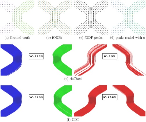
Simulated kissing dataset (SNR = 20). The left fascicle and right fascicle have a mean axon diameter of $6.88\hspace{0.17em}\hspace{0.17em}\mu \mathrm{m}$ and $2.44\hspace{0.17em}\hspace{0.17em}\mu \mathrm{m}$, respectively. (a) shows the ground truth directions used to generate the data with their length scaled by the axon diameter index α, (b) the estimated fiber ODFs (fODFs), (c) the fiber ODF peaks and (d) the fiber ODF peaks with their length scaled by α, (e) show VC and IC for AxTract, and (f) show VC and IC for conventional deterministic tractography (CDT). [Color figure can be viewed at http://wileyonlinelibrary.com]

Table 1.

Tractometer evaluation on the simulated kissing dataset

	Tractography algorithm
	Initiated from the interface						Initiated from the white matter
	AxTract			CDT			AxTract			CDT
SNR	10	20	30	10	20	30	10	20	30	10	20	30
VC	72.1	87.2	90.5	55.9	52.5	53.9	60.9	71.3	73.9	54.1	54.7	55.3
IC	15.3	8.5	7.9	31.9	42.6	44.2	19.6	15.4	15.2	27.4	32.3	34.2
NC	12.7	4.3	1.7	12.2	4.9	1.9	19.6	13.3	10.9	18.6	13.0	10.5

Tractography initialization was done both in fascicles interfaces (100 streamlines per voxel; 18,800 streamlines) and in the white matter volume (20 streamlines per voxel; 22,400 streamlines).

Table 2.

Axon diameter index α estimated on the simulated kissing dataset

	SNR	Right fascicle	Left fascicle
Ground Truth		6.88	2.44
	10	5.02 ± 0.39	3.86 ± 0.54
AxTract initiated from the interface	20	5.09 ± 0.30	3.87 ± 0.52
	30	5.08 ± 0.29	3.87 ± 0.49
	10	4.92 ± 0.49	3.79 ± 0.55
AxTract initiated from the white matter	20	5.02 ± 0.39	3.80 ± 0.53
	30	4.99 ± 0.38	3.80 ± 0.52

The ground truth and the mean α estimated on both fascicles are reported in μm (± standard deviation).

In vivo data experiment

Figures 2 and 3 show the axon diameter index α obtained with AxTract along five white matter fascicles of one subject (mgh_1001): the arcuate fasciculus (AF), the corticospinal tract (CST), the inferior fronto‐occipital fasciculus (IFOF), the superior longitudinal fasciculus (SLF), and the uncinate fasciculus (UF). In Column 3, we report the histogram of axon diameter index α estimated at each segment of all streamlines of each fascicle (streamlines shown in Column 2). In Column 5, we report for each fascicle, the histogram of the whole‐streamline median axon diameter index α (one value per streamline), for all streamlines (streamlines shown in Column 4). Differences in the estimated axon diameter index α can be observed across fascicles in both histograms. Figure 4 shows the same information for the corpus callosum (CC). The CC is split in 5 sub‐fascicles using the FreeSurfer parcellation and TractQuerier (anterior, mid‐anterior, central, mid‐posterior, posterior). A decrease in the percentage of segments with a high axon diameter index α can be observed in the posterior part of the CC. Figure 5a,b shows the CC of the same subject with AxTract streamlines colored using α estimated per segment and using the whole‐streamline median α. The largest α (green) can be observed in the central part of the CC using segment‐wise estimation. However, the trend disappears using the whole‐streamline median estimation.

Figure 2.

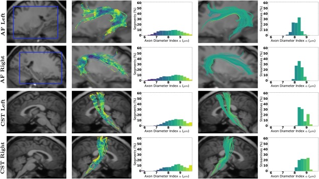
Axon diameter index α obtained with AxTract along the arcuate fasciculus (AF) and the CST. Column 1 shows a sagittal view of the T1‐weighted image with the blue squares indicating the zooming areas for streamlines visualization. Column 2 shows fascicles colored by α estimated per segment, with the histogram in Column 3. Columns 4 and 5 show, respectively, fascicles with streamlines colored by the whole‐streamline median α and the histogram of whole‐streamline median α, for all streamlines. [Color figure can be viewed at http://wileyonlinelibrary.com]

Figure 3.

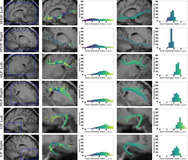
Axon diameter index α obtained with AxTract along the IFOF, the SLF, and the UF. Column 1 shows a sagittal view of the T1‐weighted image with the blue squares indicating the zooming areas for streamlines visualization. Column 2 shows fascicles colored by α estimated per segment, with the histogram in Column 3. Columns 4 and 5 show, respectively, fascicles with streamlines colored by the whole‐streamline median α and the histogram of whole‐streamline median α, for all streamlines. [Color figure can be viewed at http://wileyonlinelibrary.com]

Figure 4.

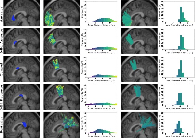
Axon diameter index α obtained with AxTract along the CC sub‐fascicles. Column 1 shows the areas used to split the fascicle. Column 2 shows sub‐fascicles colored by α estimated per segment, with the histogram in Column 3. Columns 4 and 5 show, respectively, fascicles with streamlines colored by the whole‐streamline median α and the histogram of whole‐streamline median α, for all streamlines. [Color figure can be viewed at http://wileyonlinelibrary.com]

Figure 5.

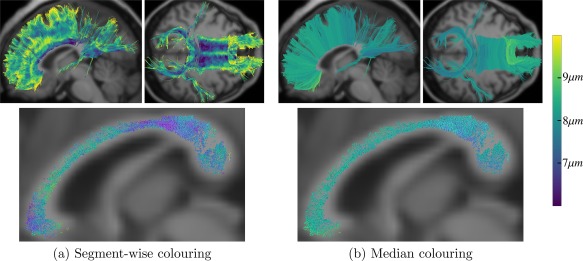
Axon diameter index α obtained with AxTract of the CC. (a,b) Streamlines colored using α estimated per segment and the whole‐streamline median α, respectively. The top row show streamlines in lateral and inferior views and the bottom row show a sagittal cut of the streamlines going through the midsagittal slice of the CC. [Color figure can be viewed at http://wileyonlinelibrary.com]

Figure 6a shows the average occurrence map of AxTract selecting a different propagation direction than CDT over the 34 subjects. AxTract changed the propagation direction more frequently in low angle crossing areas of the white matter. Areas with single fiber orientation or with multiple fiber orientations but not within the maximum deviation angle ( $\theta ={45}^{°}$) from the propagating streamline, show no changes in propagation directions. Figure 6b–d shows the segments of streamlines of three fascicles (AF, CST, UF) where such changes occurred for one subject (mgh_1001). During the tracking process of the 34 subjects, there were multiple propagation directions available in $2.5\%\pm 0.2$ of tracking steps (± standard deviation). AxTract changed the propagation direction using the axon diameter index α in $19.0\%\pm 0.3$ of tracking steps with multiple directions available.

Figure 6.

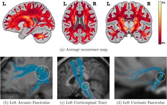
Occurrence mapping of AxTract selecting a different propagation direction than conventional deterministic tractography (CDT). (a) Average occurrence map of AxTract selecting a different propagation direction than CDT over the 34 subjects. Individual subject occurrence maps were co‐registered on the ICBM 152 average brain map, prior to the averaging. AxTract changed the propagation direction using the axon diameter index α in $19.0\%\pm 0.3$ of tracking steps with multiple directions available. (b,c,d) Occurrences of AxTract selecting a different propagating direction than CDT on three fascicles of one subject (yellow segments). The white ellipses highlight crossing areas where the use of the axon diameter index α modified the tractography. [Color figure can be viewed at http://wileyonlinelibrary.com]

Finally, Figure 7a shows the distributions of relative changes in streamlines count (%) between AxTract and CDT, across fascicles of the 34 healthy subjects: the AF, the CST, the IFOF, the SLF, the UF, and the CC. We report a significant increase in streamlines count for the CST (left: $T_{(33)}=3.9, P=7.5\times {10}^{-03}$, right: $T_{(33)}=4.0, P=5.4\times {10}^{-03}$) and for the CC (anterior: $T_{(33)}=3.4, P=2.9\times {10}^{-02}$, central: $T_{(33)}=7.1, P=6.8\times {10}^{-06}$, mid‐posterior: $T_{(33)}=5.9, P=7.1\times {10}^{-07}$, posterior: $T_{(33)}=3.1, P=2.2\times {10}^{-05}$), and a significant decrease for the AF (left: $T_{(33)}=-3.6, P=2.4\times {10}^{-02}$). Across all selected fascicles, AxTract shows an average increase 6.3% in streamline count compared to CDT. The distribution of mean α for the same fascicles is reported in Figure 7b. The mean apparent fiber density and the mean fractional anisotropy are shown as reference in Figures 7c,d. Projection and association fascicles are reported for each hemisphere. The profile of the distribution of the axon diameter index α, the apparent fiber density, and the fractional anisotropy is different and values vary across fascicles, bringing complementary information on those fascicles.

Figure 7.

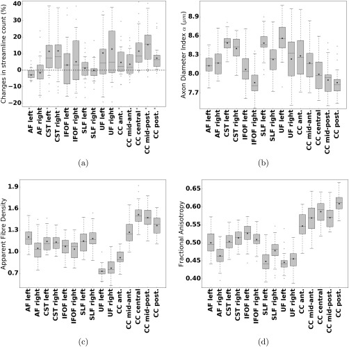
Fascicle property distributions of 34 healthy subjects. (a) Percentage change in the number of streamlines between AxTract and conventional deterministic tractography ( $\frac{AxTract-\text{CDT}}{\text{CDT}}\times 100$). Fascicle with significant increase or decrease in streamline count are marked with an asterisk ( ${}^{\ast }$). (b) The mean axon diameter index α, (c) the mean apparent fiber density, and (d) the mean fractional anisotropy, along streamline fascicles of 34 healthy subjects, obtained with AxTract. Results are shown for six fascicles: the arcuate fasciculus (AF), the CST, the IFOF, the SLF, the UF, and the CC. The CC is split in five sub‐fascicles using the FreeSurfer parcellation (anterior, mid‐anterior, central, mid‐posterior, posterior) and TractQuerier. Projection and association fascicles are reported for each hemisphere. The black line indicates the median, the square indicates the mean, the box extends from the first and third quartile and the whiskers are at the 5th and 95th percentile of the distribution.

DISCUSSION

We introduced a novel tractography method, AxTract, which incorporates apparent axonal microstructure measurements to reconstruct white matter fascicles of the brain. Despite the current discussion on the feasibility of measuring axon diameters with DW‐MRI [Alexander et al., 2010; Novikov et al., 2014], our results show that incorporating surrogate measures to axon diameter has a positive effect on tractography results. Specifically, we incorporated the axon diameter index α [Alexander et al., 2010] obtained from DW‐MRI using the efficient implementation AMICO [Auría et al., 2015]. Using this technique, our algorithm can disentangle complex architecture based on microstructure characteristics. AxTract is able to distinguish white matter fascicles through their microstructure characteristics while being able to perform full brain tractography in reasonable time (approximately 72 h for AxTract compared to 6 h for the CDT implementation, for 600,000 streamlines). Our results on simulated data show that AxTract is a promising approach to reduce the incidence of IC produced by current tractography algorithms. Our results on in vivo data show that the axon diameter index α changed the direction of the tracking resulting in an overall increase of the number of streamlines in the identified fascicles. In the absence of ground truth in vivo connectivity data, it is a challenge to show the increase of VC and decrease of IC but, we show evidence that AxTract is a novel method taking a step in the right direction.

Reducing ambiguities in complex white matter architecture

AxTract distinguishes fascicles in complex architectures when these have different axon diameter. Specifically, in the crossing area on Figure 1, AxTract privileges following the direction which minimizes the deviation from axon diameter index α of the fascicle being reconstructed while the usual tractography approach is to minimize the angular deviation. In doing so, AxTract is able to better resolve the kissing configuration and decreases the percentage of IC. Always following the direction with the lowest local angular deviation, as with CDT, leads to errors in the kissing configuration reconstruction. This is quantitatively reported by the Tractometer [Côté et al., 2013] metrics in Table 1. AxTract always increases the VC and decreases the IC compared to CDT. The VC also increase with an increase in SNR for AxTract. The increase in VC is also higher for AxTract initiating the tractography from fascicle extremities, that is, the white matter/gray matter interface. This is because the tracking starts in regions where α is specific of the fascicle, that is, α_d estimated in the initial direction tend toward the ground truth α of the fascicle. This is not the case when the tracking starts in the central part of the dataset, where only one peak is obtained from the fiber ODF. Hence, AMICO estimates the axon diameter index in this single direction, despite the ground truth having two directions, see Figure 1a,c. As the two ground truth directions are almost aligned, the axon diameter index tends toward the average α of both simulated fascicles. This makes AxTract unable to distinguish which direction to follow in subsequent tractography steps with multiple fiber ODF peaks. Nonetheless, AxTract performs similarly to the CDT when initiated in regions where fascicles population cannot be distinguished. It is worth mentioning that two streamlines being reconstructed with AxTract, reaching the very same position and with the same previous tracking direction would not necessarily result in the same trajectory. Contrary to CDT, AxTract uses the information from many previous tracking steps (up to 5 cm with ${\alpha }_{\rho }$) to select the propagation direction.

The estimated axon diameter index α along streamlines is different in the two fascicles, but similar across SNR and tractography initialization techniques (see Table 2). However, α is always underestimated for the fascicle with the highest cylinder diameter, and overestimated for the fascicle with the lowest cylinder diameter. Although the cylinder diameter estimated at each segment is not the same as the ground truth, the estimation is consistent across segment and streamlines of the same fascicle. This can be observed in Figure 1d where the fiber ODF peaks have a consistent α estimation with AMICO [Auría et al., 2015], both in single and multiple fibers populations. Table 2 shows that at high SNR, the standard deviation of the estimation of the axon diameter index α decreases. This decrease in the variability of the estimated α increases the overall quality of the tractography reconstruction, as shown by the Tractometer in Table 1. This stresses the importance of having high SNR data for microstructure estimation and consequently, microstructure informed tractography. Nevertheless, AxTract always increases VC and decreases IC compared to CDT, even at SNR = 10.

Characterizing axon diameter index in vivo

AxTract enables the characterization of the axon diameter index α along white matter fascicles in vivo. The estimation of α with AMICO [Auría et al., 2015] along the tracking process with AxTract seems to be spatially coherent, as shown in Figures 2, 3, and 4, both on local estimation and on the median along streamlines. The value observed in the CC, see Figure 5a, follows the low‐high‐low trend observed in histology [Aboitiz et al., 1992], with lower values in the splenium and genu, and higher value in the body of the CC. However, as shown in Figures 5, this is visible only in the midsagittal slice of the CC. Alexander et al. [2010] suggested the trend observed in the midsagittal slice could be related to more complex axon geometry within those voxels, such as bending and fanning, not well supported by the ActiveAx model, and biasing the fitting. The ActiveAx model was later extended by Zhang et al. [2011b] to account for orientation dispersion using a Watson distribution. Their method better explains the data for the considered voxels, providing equally or more consistent agreement between the microstructure estimated and the observations from histology [Zhang et al., 2011b]. Nonetheless, similar estimates of the axon diameter index α were obtained for the midsagittal slice of the CC with the proposed model of the axonal dispersion. Recently, Ronen et al. [2013] reported axonal angular dispersion in the body of the CC that could bias the estimation of the axon diameter index α. This bias could also be a partial explanation for the discrepancy between the relative differences in the average α of different fascicles, shown in Figure 7b, and the histological measures done by Liewald et al. [2014]. This could also be due to the limitation of histology which only allows for measuring axon diameters on a single slice [Liewald et al., 2014] while AxTract enables the overall quantification on the whole fascicle. Further investigation is needed to better understand why microstructure trends on whole fascicles differ from trends on a single slice, as well as the relationship between the axon diameter index α and axon physiology [Aboitiz et al., 1992; Alexander et al., 2010; Daducci et al., 2015; Debanne et al., 2011; Dyrby et al., 2012; Liewald et al., 2014; Ye et al., 2016; Zhang et al., 2011b]. Remarkably, AxTract, despite these limitations, is able to show consistent differences between fascicles in the mean axon diameter index α segment‐wise across subjects (see Fig. 7b). Fascicles mean axon diameter index can also be computed a posteriori from the axon diameter index in the segment‐wise orientation of streamlines obtained from CDT. Additionally, fascicles mean axon diameter index can be obtained from streamline post‐processing methods such as MicroTrack [Sherbondy et al., 2010] or COMMIT [Barakovic et al., 2016; Daducci et al., 2014]. These methods associate a white matter model to each streamline and optimize the model parameters of all streamlines simultaneously to best fit the DW‐MRI signal. They rely on the same hypothesis that microstructure features are consistent along the white matter fibers. In both cases, this provide an additional fascicle index that could be studied alongside other indices such as the apparent fiber density and the fractional anisotropy, to improve our understanding of brain connectivity and pathology.

Toward reducing IC in vivo

The axon diameter index α changed the tracking direction mostly in voxels located in low angle crossing areas of the white matter, as shown on Figure 6. On average, these changes in direction happened in 19.0% of tracking steps with multiple directions available, which account for 2.5% of all tracking steps. This suggests that the direction picked by the CDT is usually the direction that shows the less variation in α. Nonetheless, a single change in the propagation direction can affect the reconstruction of the whole fascicle. This is shown in Figure 7a, where AxTract increases the streamline count by an average of 6.3% across the selected fascicles for 34 subjects. This increase is obtained by solely changing the selection of the propagation direction with AxTract, keeping the same other tractography parameters. This increase in streamline count for a fascicle can be explained by three factors: (1) a decrease in erroneous streamlines not reaching the gray matter, (2) a decrease in erroneous streamlines connecting invalid gray matter regions, or (3) streamlines connecting alternative valid gray matter regions from initial positions. Both factors (1) and (2) will improve the streamline reconstruction by overall increasing the VC. However, the observed increase of VC could be due to a decrease in VCs from other existing fascicles of the brain (factor 3). We observed such a decrease in the streamline count for the AF, see Figure 7a. Seeds forming AF connections with CDT might have formed other VC with AxTract (e.g., fascicles kissing or crossing with the AF such as the SLF). This reduction in the streamline count might also be attributed to more seeds forming IC or erroneous streamlines due to errors in the axon diameter index estimation, making AxTract follow incorrect directions. Further investigation is needed to better understand the changes in the streamlines distribution in vivo. Nevertheless, this suggests that AxTract has a consistent effect on some of the reported fascicles across subjects. More realistic phantoms, such the one proposed for the ISMRM 2015 Tractography challenge (http://tractometer.org/ismrm_2015http://_challenge) [Maier‐Hein et al., 2017] should also provide more insights in the potential of AxTract.

It is worth mentioning that we observed fascicles in some subjects with lower streamline coverage than we expected for both AxTract and the CDT (e.g., the mid‐posterior part of the CC and the right IFOF of subject mgh_1001). In most cases, there were streamlines covering the expected fascicles area. However, these streamlines did not fully agree the strict fascicles definition used to automatically obtained streamlines with TractQuerier (e.g., incomplete streamlines stopping in the white matter).

Limitations and future work

In the current implementation, the propagation direction is selected only by minimizing the change in the axon diameter index, given the directions within the maximum deviation angle θ. It is not clear which angle θ provides the optimal reconstruction throughout fascicles of the brain. It would be interesting to relax the angular criterion, especially with AxTract where two criteria (difference in axon diameter index and angular difference) are used in the selection of the propagation direction. In future work, AxTract could be extended to select the propagation direction using a distance function combining both criteria (e.g., allowing high angular difference when the distance in axon diameter index is low).

AxTract approximates the axon diameter index of the fascicle being reconstructed using the median segment‐wise α over a fixed distance of 5 cm. This parameter is of high importance as it affects the propagation direction selected by AxTract. If the distance parameter is too little, fascicles overlapping with the one being reconstructed will bias its axon diameter index estimation. This will cause the tractography to potentially follow erroneous propagation directions. Alternatively, if the distance parameter is too big, biological changes in the fascicle axon diameter distribution cannot be taking into account (e.g., branching or fanning). Again, this could lead to the tractography following erroneous directions. More research is needed to best select and adapt this parameter for the fascicle being reconstructed.

Finally, AxTract will directly benefit from improvements in local axon diameter acquisition, modeling, and reconstruction techniques. In future work, it will be of interest to extend the current tracking algorithm to follow not only the median α of the fascicle, but to follow the α distribution of a fascicle [Assaf et al., 2008]. In particular, fascicles have a distribution of axon diameter that can partially overlaps, crosses and branches with other fascicles. Following the direction with the lowest change in α can results in an under‐representation (or absence) of the smaller branching parts of the reconstructed fascicles. AxTract follows the directions having the most coherence in α, and as such, aims at reconstructing the main structure of the fascicles. Further improvements in the axon diameter distribution mapping could allow tractography to disentangle fascicles axon diameter distribution overlapping in a parallel direction and helps identify smaller branching structures. In addition, the estimation of α could be extended to more directions than the fiber ODF peaks. This requires new developments in axon diameter mapping methods, but would allow the use of α in probabilistic tractography algorithms [e.g., Behrens et al., 2007; Jeurissen et al., 2011] or global tractography frameworks [e.g., Fillard et al., 2009; Jbabdi et al., 2007; Kreher et al., 2008; Reisert et al., 2011, 2014].

CONCLUSION

To conclude, we presented AxTract, a novel algorithm to address the crossing/kissing problem of fascicles passing through areas of complex white matter configurations. AxTract uses axon diameter information to reduce ambiguities in the selection of the propagation direction, thus potentially reducing IC and increasing VC produced by tractography algorithms. This was shown on simulations and on a group of 34 healthy subjects. AxTract is a framework and the first step toward advanced techniques able to incorporate tractography and microstructure imaging together. As microstructure modeling and reconstruction improve in the future, so will AxTract. This will enable the study of microstructure characteristics of white matter fascicles and go toward quantitative connectivity mapping.

Supporting information

Supporting Information

AXON DIAMETER INDEX ESTIMATION

The framework AMICO [Auría et al., 2015; Daducci et al., 2015] provides the means to efficiently estimates microstructure information using a linear formulation. AMICO expresses the multi‐compartment mapping problem as

$$\begin{array}{c}\frac{\mathit{S}}{S_0}=\mathrm{\Phi }\mathbf{x}+\mathit{\eta },\hfill \end{array}$$

where $\mathit{S}\in {ℝ}^N$ is the vector of diffusion weighted signal measurements, S ₀ the signal without diffusion weighting, $\mathbf{x}\in {ℝ}^K$ the coefficients of the dictionary $\mathrm{\Phi }\in {ℝ}^{N\times K}$ and $\mathit{\eta }\in {ℝ}^N$ the acquisition noise [Daducci et al., 2015]. The dictionary $\mathrm{\Phi }$ is built from different matrices:

$$\begin{array}{c}\mathrm{\Phi }=[{\mathrm{\Phi }}^{\text{iso}}| {\mathrm{\Phi }}_1^{\text{intra}}| {\mathrm{\Phi }}_1^{\text{extra}}|\dots | {\mathrm{\Phi }}_M^{\text{intra}}| {\mathrm{\Phi }}_M^{\text{extra}}],\hfill \end{array}$$

where ${\mathrm{\Phi }}^{\text{iso}}\in {ℝ}^{N\times K_{\text{iso}}}$ are isotropic response functions accounting for free and isotropically restricted water [Panagiotaki et al., 2012] with diffusivity ranging from $3\times {10}^{-3}$ to $1\times {10}^{-3}$ ${\text{mm}}^2/\mathrm{s}$, and ${\mathrm{\Phi }}_i^{\text{intra}}\in {ℝ}^{N\times K_{\text{intra}}}$ the intra‐axonal and ${\mathrm{\Phi }}_i^{\text{extra}}\in {ℝ}^{N\times K_{\text{extra}}}$ extra‐axonal compartments to account for the DW‐MRI signal attenuation along the M fiber directions ${\mathit{d}}_m$. The intra‐axonal compartments ${\mathrm{\Phi }}_i^{\text{intra}}$ models the DW‐MRI signal decay of water molecules restricted within parallel cylinders [Alexander et al., 2010; Daducci et al., 2015; Dyrby et al., 2012; Panagiotaki et al., 2012] of diameter ranging from 2 to 10 μm. The intra‐axonal diffusivity was fixed to $1.7\times {10}^{-3}$ ${\text{mm}}^2/\mathrm{s}$ [Dyrby et al., 2012; Panagiotaki et al., 2012]. The parallel diffusivity of the extra‐axonal compartments ${\mathrm{\Phi }}_i^{\text{extra}}$ was also fixed to $1.7\times {10}^{-3}$ ${\text{mm}}^2/\mathrm{s}$, and distinct perpendicular diffusivity ranging from $0.06\times {10}^{-3}$ to $0.42\times {10}^{-3}$ ${\text{mm}}^2/\mathrm{s}$ [Daducci et al., 2013; Panagiotaki et al., 2012]. The model assumes no exchange between compartments.

Given the DW‐MRI signal and a set of fiber directions, AMICO solves

$$\begin{array}{c}\arg \underset{{}_{\mathbf{x}\ge 0}}{\min }\frac{1}{2}{\left|\right|\mathrm{\Phi }\mathbf{x}-\frac{\mathit{S}}{S_0}\left|\right|}_2^2+\lambda \frac{1}{2}\left|\right|\mathbf{x}|{|}_2^2,\hspace{1em}\mathrm{s}.\mathrm{t}. \lambda >0\hfill \end{array}$$

where $\left|\right|·|{|}_2^2$ is the ${\ell }_2$ norm and the parameter λ controls the trade‐off between the data and the regularization terms. Doing so, it enables the estimation of the mean diameter of cylinders along each fiber direction

$$\begin{array}{c}{\alpha }_{{\mathit{d}}_m}=\frac{\sum _{j}2R_j{\mathbf{x}}_{i_j}^{\text{intra}}}{\sum _j{\mathbf{x}}_{i_j}^{\text{intra}}},\hfill \end{array}$$

where ${\mathbf{x}}_{i_j}^{\text{intra}}$ is the volume fraction of the compartment ${\mathrm{\Phi }}_{i_j}^{\text{intra}}$ corresponding to cylinder of radius R_j (μm) in the direction ${\mathit{d}}_m$. AMICO uses up to three fiber directions in the estimation [Auría et al., 2015]. We refer to ${\alpha }_{{\mathit{d}}_m}$ as the axon diameter index [Alexander et al., 2010; Auría et al., 2015; Dyrby et al., 2012].

REFERENCES

- Aboitiz F, Scheibel AB, Fisher RS, Zaidel E (1992): Fiber composition of the human corpus callosum. Brain Res 598:143–153. [DOI] [PubMed] [Google Scholar]
- Alexander DC, Hubbard PL, Hall MG, Moore EA, Ptito M, Parker GJ, Dyrby TB (2010): Orientationally invariant indices of axon diameter and density from diffusion MRI. NeuroImage 42:1374–1389. [DOI] [PubMed] [Google Scholar]
- Amitay SB, Lifshits S, Barazany D, Assaf Y (2016): 3‐Dimensional Axon Diameter Estimation of White Matter Fiber Tracts in The Human Brain. Geneva, Switzerland: Organization for Human Brain Mapping.
- Andersson J, Xu J, Yacoub E, Auerbach E, Moeller S, Ugurbil K (2012): A comprehensive Gaussian Process framework for correcting distortions and movements in diffusion images. In: International Symposium on Magnetic Resonance in Medicine. Melbourne, Australia.
- Assaf Y, Basser PJ (2005): Composite hindered and restricted model of diffusion (CHARMED) MR imaging of the human brain. NeuroImage 27:48–58. [DOI] [PubMed] [Google Scholar]
- Assaf Y, Blumenfeld‐Katzir T, Yovel Y, Basser PJ (2008): AxCaliber: A method for measuring axon diameter distribution from diffusion MRI. Magn Reson Med 59:1347–1354. [DOI] [PMC free article] [PubMed] [Google Scholar]
- Auría AR, Romascano DPR, Canales‐Rodriguez E, Wiaux Y, Dyrby TB, Alexander D, Thiran J‐P, Daducci A (2015): Accelerated microstructure imaging via convex optimisation for regions with multiple fibres (amicox). In: IEEE International Conference on Image Processing, Québec, Canada.
- Avants BB, Tustison N, Song G (2009): Advanced normalization tools (ants). Insight J 2:1–35. [Google Scholar]
- Barakovic M, Romascano D, Dyrby T, Alexander D, Descoteaux M, Jean‐Philippe Thiran AD (2016): Assessment of Bundle‐Specific Axon Diameter Distributions Using Diffusion MRI Tractography. Geneva, Switzerland: Organization for Human Brain Mapping.
- Barazany D, Jones DK, Assaf Y (2011): AxCaliber 3D. In: International Symposium on Magnetic Resonance in Medicine, Montréal, Canada.
- Basser PJ, Pajevic S, Pierpaoli C, Duda J, Aldroubi A (2000): In vivo fiber tractography using DT‐MRI data. Magn Reson Med 44:625–632. [DOI] [PubMed] [Google Scholar]
- Behrens TEJ, Berg HJ, Jbabdi S, Rushworth MFS, Woolrich MW (2007): Probabilistic diffusion tractography with multiple fibre orientations: What can we gain? NeuroImage 34:144–155. [DOI] [PMC free article] [PubMed] [Google Scholar]
- Burcaw LM, Fieremans E, Novikov DS (2015): Mesoscopic structure of neuronal tracts from time‐dependent diffusion. NeuroImage 114:18–37. [DOI] [PMC free article] [PubMed] [Google Scholar]
- Caruyer E, Daducci A, Descoteaux M, Houde J‐C, Thiran J‐P, Verma R (2014): Phantomas: A flexible software library to simulate diffusion MR phantoms. In: International Symposium on Magnetic Resonance in Medicine, Milan, Italy.
- Catani M, Allin MPG, Husain M, Pugliese L, Mesulam MM, Murray RM, Jones DK (2007): Symmetries in human brain language pathways correlate with verbal recall. Proc Natl Acad Sci USA 104:17163–17168. [DOI] [PMC free article] [PubMed] [Google Scholar]
- Côté M‐A, Girard G, Boré A, Garyfallidis E, Houde J‐C, Descoteaux M (2013): Tractometer: Towards validation of tractography pipelines. Med Image Anal 17:844–857. [DOI] [PubMed] [Google Scholar]
- Daducci A, Dal Palu A, Lemkaddem A, Thiran J‐P (2013): A convex optimization framework for global tractography. In: IEEE International Symposium on Biomedical Imaging. San Francisco, US, pp 524–527.
- Daducci A, Dal Palu A, Alia L, Thiran J‐P (2014): COMMIT: Convex optimization modeling for micro‐structure informed tractography. IEEE Trans Med Imaging 34:246–257. [DOI] [PubMed] [Google Scholar]
- Daducci A, Canales‐Rodríguez EJ, Zhang H, Dyrby TB, Alexander DC, Thiran J‐P (2015): Accelerated Microstructure Imaging via Convex Optimization (AMICO) from diffusion MRI data. NeuroImage 105:32–44. [DOI] [PubMed] [Google Scholar]
- Daducci A, Dal Palú A, Descoteaux M, Thiran J‐P (2016): Microstructure informed tractography: Pitfalls and open challenges. Front Neurosci 10:247. [DOI] [PMC free article] [PubMed] [Google Scholar]
- Debanne D, Campanac E, Bialowas A, Carlier E, Alcaraz G (2011): Axon physiology. Physiol Rev 91:555–602. [DOI] [PubMed] [Google Scholar]
- Dell'Acqua F, Rizzo G, Scifo P, Clarke RA, Scotti G, Fazio F (2007): A model‐based deconvolution approach to solve fiber crossing in diffusion‐weighted MR imaging. IEEE Trans Biomed Eng 54:462–472. [DOI] [PubMed] [Google Scholar]
- Dell'Acqua F, Simmons A, Williams S, Catani M (2010): Can Spherical Deconvolution give us more information beyond fibre orientation? Towards novel quantifications of white matter integrity. In: International Symposium on Magnetic Resonance in Medicine, Stockholm, Sweden.
- Dell'Acqua F, Simmons A, Williams SC, Catani M (2013): Can spherical deconvolution provide more information than fiber orientations? Hindrance modulated orientational anisotropy, a true‐tract specific index to characterize white matter diffusion. Hum Brain Mapp 34:2464–2483. [DOI] [PMC free article] [PubMed] [Google Scholar]
- Descoteaux M, Angelino E, Fitzgibbons S, Deriche R (2007): Regularized, fast, and robust analytical Q‐ball imaging. Magn Reson Med 58:497–510. [DOI] [PubMed] [Google Scholar]
- Descoteaux M, Deriche R, Knösche TR, Anwander A (2009): Deterministic and probabilistic tractography based on complex fibre orientation distributions. IEEE Trans Med Imaging 28:269–286. [DOI] [PubMed] [Google Scholar]
- Dyrby TB, Sø gaard LV, Hall MG, Ptito M, Alexander DC (2012): Contrast and stability of the axon diameter index from microstructure imaging with diffusion MRI. Magn Reson Med 721:711–721. [DOI] [PMC free article] [PubMed] [Google Scholar]
- Fan Q, Witzel T, Nummenmaa A, Van Dijk KR, Van Horn JD, Drews MK, Somerville LH, Sheridan MA, Santillana RM, Snyder J, Hedden T, Shaw EE, Hollinshead MO, Renvall V, Zanzonico R, Keil B, Cauley S, Polimeni JR, Tisdall D, Buckner RL, Wedeen VJ, Wald LL, Toga AW, Rosen BR (2016): MGHUSC Human Connectome Project datasets with ultra‐high b‐value diffusion MRI. NeuroImage 124:1108–1114. [DOI] [PMC free article] [PubMed] [Google Scholar]
- Fick RHJ, Wassermann D, Caruyer E, Deriche R (2016): MAPL: Tissue microstructure estimation using Laplacian‐regularized MAP‐MRI and its application to HCP data. NeuroImage 134:365–385. [DOI] [PubMed] [Google Scholar]
- Fillard P, Poupon C, Mangin J‐F (2009): A novel global tractography algorithm based on an adaptive spin glass model. In: International Conference on Medical Image Computing and Computer Assisted Intervention, London, United Kingdom. pp 927–934. [DOI] [PubMed]
- Fonov V, Evans AC, Botteron K, Almli CR, McKinstry RC, Collins DL (2011): Unbiased average age‐appropriate atlases for pediatric studies. NeuroImage 54:313–327. [DOI] [PMC free article] [PubMed] [Google Scholar]
- Garyfallidis E, Brett M, Amirbekian B, Rokem A, Van Der Walt S, Descoteaux M, Nimmo‐Smith I (2014): Dipy, a library for the analysis of diffusion MRI data. Front Neuroinform 8:8. [DOI] [PMC free article] [PubMed] [Google Scholar]
- Girard G, Whittingstall K, Deriche R, Descoteaux M (2014): Towards quantitative connectivity analysis: Reducing tractography biases. NeuroImage 98:266–278. [DOI] [PubMed] [Google Scholar]
- Greve DN, Fischl B (2009): Accurate and robust brain image alignment using boundary‐based registration. NeuroImage 48:63–72. [DOI] [PMC free article] [PubMed] [Google Scholar]
- Gudbjartsson H, Patz S (1995): The Rician distribution of noisy MRI data. Magn Reson Med 34:910–914. [DOI] [PMC free article] [PubMed] [Google Scholar]
- Hall MG, Alexander DC (2009): Convergence and parameter choice for Monte‐Carlo simulations of diffusion MRI. IEEE Trans Med Imaging 28:1354–1364. [DOI] [PubMed] [Google Scholar]
- Huang SY, Nummenmaa A, Witzel T, Duval T, Cohen‐Adad J, Wald LL, McNab JA (2015): The impact of gradient strength on in vivo diffusion MRI estimates of axon diameter. NeuroImage 106:464–472. [DOI] [PMC free article] [PubMed] [Google Scholar]
- Jbabdi S, Woolrich MW, Andersson JLR, Behrens TEJ (2007): A Bayesian framework for global tractography. NeuroImage 37:116–129. [DOI] [PubMed] [Google Scholar]
- Jbabdi S, Sotiropoulos SN, Haber SN, Van Essen DC, Behrens TE (2015): Measuring macroscopic brain connections in vivo. Nat Neurosci 18:1546–1555. [DOI] [PubMed] [Google Scholar]
- Jeurissen B, Leemans A, Jones DKDK, Tournier J‐DJD, Sijbers J (2011): Probabilistic fiber tracking using the residual bootstrap with constrained spherical deconvolution. Hum Brain Mapp 32:461–479. [DOI] [PMC free article] [PubMed] [Google Scholar]
- Jolles D, Wassermann D, Chokhani R, Richardson J, Tenison C, Bammer R, Fuchs L, Supekar K, Menon V (2016): Plasticity of left perisylvian white‐matter tracts is associated with individual differences in math learning. Brain Struct Funct 221:1337–1351. [DOI] [PMC free article] [PubMed] [Google Scholar]
- Jones DK (2010): Challenges and limitations of quantifying brain connectivity in vivo with diffusion MRI. Imaging Med 2:341–355. [Google Scholar]
- Kaden E, Kruggel F, Alexander DC (2015): Quantitative mapping of the per‐axon diffusion coefficients in brain white matter. Magn Reson Med 75:1752–1763. [DOI] [PMC free article] [PubMed] [Google Scholar]
- Keil B, Blau JN, Biber S, Hoecht P, Tountcheva V, Setsompop K, Triantafyllou C, Wald LL (2013): A 64‐channel 3T array coil for accelerated brain MRI. Magn Reson Med 70:248–258. [DOI] [PMC free article] [PubMed] [Google Scholar]
- Kreher BW, Mader I, Kiselev VG (2008): Gibbs tracking: A novel approach for the reconstruction of neuronal pathways. Magn Reson Med 60:953–963. [DOI] [PubMed] [Google Scholar]
- Lebel C, Beaulieu C (2009): Lateralization of the arcuate fasciculus from childhood to adulthood and its relation to cognitive abilities in children. Hum Brain Mapp 30:3563–3573. [DOI] [PMC free article] [PubMed] [Google Scholar]
- Liewald D, Miller R, Logothetis N, Wagner H‐J, Schüz A (2014): Distribution of axon diameters in cortical white matter: An electron‐microscopic study on three human brains and a macaque. Biol Cybern 108:541–557. [DOI] [PMC free article] [PubMed] [Google Scholar]
- Maier‐Hein K, Neher P, Houde J‐C, Cote M‐A, Garyfallidis E, Zhong J, Chamberland M, Yeh F‐C, Lin YC, Ji Q, Reddick WE, Glass JO, Chen DQ, Feng Y, Gao C, Wu Y, Ma J, Renjie H, Li Q, Westin C‐F, Deslauriers‐Gauthier S, Gonzalez JOO, Paquette M, St‐Jean S, Girard G, Rheault F, Sidhu J, Tax CMW, Guo F, Mesri HY, David S, Froeling M, Heemskerk AM, Leemans A, Bore A, Pinsard B, Bedetti C, Desrosiers M, Brambati S, Doyon J, Sarica A, Vasta R, Cerasa A, Quattrone A, Yeatman J, Khan AR, Hodges W, Alexander S, Romascano D, Barakovic M, Auria A, Esteban O, Lemkaddem A, Thiran J‐P, Cetingul HE, Odry BL, Mailhe B, Nadar M, Pizzagalli F, Prasad G, Villalon‐Reina J, Galvis J, Thompson P, Requejo F, Laguna P, Lacerda L, Barrett R, Dell'Acqua F, Catani M, Petit L, Caruyer E, Daducci A, Dyrby T, Holland‐Letz T, Hilgetag C, Stieltjes B, Descoteaux M (2017): The challenge of mapping the human connectome based on diffusion tractography. Nat Commun, in press. [DOI] [PMC free article] [PubMed] [Google Scholar]
- Malcolm JG, Shenton ME, Rathi Y (2010): Filtered multitensor tractography. IEEE Trans Med Imaging 29:1664–1675. [DOI] [PMC free article] [PubMed] [Google Scholar]
- Matsui JT, Vaidya JG, Wassermann D, Kim RE, Magnotta VA, Johnson HJ, Paulsen JS (2015): Prefrontal cortex white matter tracts in prodromal Huntington disease. Hum Brain Mapp 36:3717–3732. [DOI] [PMC free article] [PubMed] [Google Scholar]
- Novikov DS, Jensen JH, Helpern JA, Fieremans E (2014): Revealing mesoscopic structural universality with diffusion. Proc Natl Acad Sci USA 111:5088–5093. [DOI] [PMC free article] [PubMed] [Google Scholar]
- Özarslan E, Koay CG, Shepherd TM, Komlosh ME, İrfanoğlu MO, Pierpaoli C, Basser PJ (2013): Mean apparent propagator (MAP) MRI: A novel diffusion imaging method for mapping tissue microstructure. NeuroImage 78:16–32. [DOI] [PMC free article] [PubMed] [Google Scholar]
- Panagiotaki E, Schneider T, Siow B, Hall MG, Lythgoe MF, Alexander DC (2012): Compartment models of the diffusion MR signal in brain white matter: A taxonomy and comparison. NeuroImage 59:2241–2254. [DOI] [PubMed] [Google Scholar]
- Pestilli F, Yeatman JD, Rokem A, Kay KN, Wandell BA (2014): Evaluation and statistical inference for human connectomes. Nat Methods 11:1058–1063. [DOI] [PMC free article] [PubMed] [Google Scholar]
- Raffelt D, Tournier J‐D, Rose S, Ridgway GR, Henderson R, Crozier S, Salvado O, Connelly A (2012): Apparent Fibre Density: A novel measure for the analysis of diffusion‐weighted magnetic resonance images. NeuroImage 59:3976–3994. [DOI] [PubMed] [Google Scholar]
- Reisert M, Mader I, Anastasopoulos C, Weigel M, Schnell S, Kiselev V (2011): Global fiber reconstruction becomes practical. NeuroImage 54:955–962. [DOI] [PubMed] [Google Scholar]
- Reisert M, Kiselev VG, Dihtal B, Kellner E, Novikov DS (2014): MesoFT: Unifying diffusion modelling and fiber tracking. In: International Conference on Medical Image Computing and Computer‐Assisted Intervention, Boston, United‐States. pp 201–208. [DOI] [PMC free article] [PubMed]
- Ritchie JM (1982): On the relation between fibre diameter and conduction velocity in myelinated nerve fibres. Proc R Soc Lond Ser B Biol Sci 217:29–35. [DOI] [PubMed] [Google Scholar]
- Ronen I, Budde M, Ercan E, Annese J, Techawiboonwong A, Webb A (2013): Microstructural organization of axons in the human corpus callosum quantified by diffusion‐weighted magnetic resonance spectroscopy of N‐acetylaspartate and post‐mortem histology. Brain Struct Funct 219:1773–1785. [DOI] [PubMed] [Google Scholar]
- Salat DH, Greve DN, Pacheco JL, Quinn BT, Helmer KG, Buckner RL, Fischl B (2009): Regional white matter volume differences in nondemented aging and Alzheimer's disease. NeuroImage 44:1247–1258. [DOI] [PMC free article] [PubMed] [Google Scholar]
- Savadjiev P, Rathi Y, Bouix S, Smith AR, Schultz RT, Verma R, Westin C‐F (2014): Fusion of white and gray matter geometry: A framework for investigating brain development. Med Image Anal 18:1349–1360. [DOI] [PMC free article] [PubMed] [Google Scholar]
- Scherrer B, Schwartzman A, Taquet M, Sahin M, Prabhu SP, Warfield SK (2015): Characterizing brain tissue by assessment of the distribution of anisotropic microstructural environments in diffusion‐compartment imaging (DIAMOND). Magn Reson Med 76:963–977. [DOI] [PMC free article] [PubMed] [Google Scholar]
- Sepehrband F, Clark KA, Ullmann JFP, Kurniawan ND, Leanage G, Reutens DC, Yang Z (2015): Brain tissue compartment density estimated using diffusion‐weighted MRI yields tissue parameters consistent with histology. Hum Brain Mapp 36:3687–3702. [DOI] [PMC free article] [PubMed] [Google Scholar]
- Setsompop K, Kimmlingen R, Eberlein E, Witzel T, Cohen‐Adad J, McNab JA, Keil B, Tisdall MD, Hoecht P, Dietz P, Cauley SF, Tountcheva V, Matschl V, Lenz VH, Heberlein K, Potthast A, Thein H, Van Horn J, Toga A, Schmitt F, Lehne D, Rosen BR, Wedeen V, Wald LL (2013): Pushing the limits of in vivo diffusion MRI for the Human Connectome Project. NeuroImage 80:220–233. [DOI] [PMC free article] [PubMed] [Google Scholar]
- Sherbondy AJ, Rowe MC, Alexander DC (2010): MicroTrack: An algorithm for concurrent projectome and microstructure estimation. In: International Conference on Medical Image Computing and Computer‐Assisted Intervention, Beijing, China. pp 183–90 [DOI] [PubMed]
- Smith RE, Tournier J‐D, Calamante F, Connelly A (2013): SIFT: Spherical‐deconvolution informed filtering of tractograms. NeuroImage 67:298–312. [DOI] [PubMed] [Google Scholar]
- Song S‐K, Yoshino J, Le TQ, Lin S‐J, Sun S‐W, Cross AH, Armstrong RC (2005): Demyelination increases radial diffusivity in corpus callosum of mouse brain. NeuroImage 26:132–140. [DOI] [PubMed] [Google Scholar]
- Thiebaut de Schotten M, Ffytche DH, Bizzi A, Dell'Acqua F, Allin M, Walshe M, Murray R, Williams SC, Murphy DG, Catani M (2011): Atlasing location, asymmetry and inter‐subject variability of white matter tracts in the human brain with MR diffusion tractography. NeuroImage 54:49–59. [DOI] [PubMed] [Google Scholar]
- Thomas C, Ye FQ, Irfanoglu MO, Modi P, Saleem KS, Leopold DA, Pierpaoli C (2014): Anatomical accuracy of brain connections derived from diffusion MRI tractography is inherently limited. Proc Natl Acad Sci USA 111:16574–16579. [DOI] [PMC free article] [PubMed] [Google Scholar]
- Tournier J‐D, Calamante F, Connelly A (2007): Robust determination of the fibre orientation distribution in diffusion MRI: Non‐negativity constrained super‐resolved spherical deconvolution. NeuroImage 35:1459–1472. [DOI] [PubMed] [Google Scholar]
- Tournier J‐D, Calamante F, Connelly A (2012): MRtrix: Diffusion tractography in crossing fiber regions. Int J Imaging Syst Technol 22:53–66. [Google Scholar]
- Tristán‐Vega A, Westin C‐F, Aja‐Fernández S (2009): Estimation of fiber orientation probability density functions in high angular resolution diffusion imaging. NeuroImage 47:638–650. [DOI] [PubMed] [Google Scholar]
- Tuch D (2004): Q‐ball imaging. Magn Reson Med 52:1358–1372. [DOI] [PubMed] [Google Scholar]
- Vernooij MW, Smits M, Wielopolski PA, Houston GC, Krestin GP, Van Der Lugt A (2006): Fiber density asymmetry of the arcuate fasciculus in relation to functional hemispheric language lateralization in both right‐ and left‐handed healthy subjects: A combined fMRI and DTI study. NeuroImage 35:1064–1076. [DOI] [PubMed] [Google Scholar]
- Wassermann D, Makris N, Rathi Y, Shenton M, Kikinis R, Kubicki M, Westin C‐F (2016): The white matter query language: A novel approach for describing human white matter anatomy. Brain Struct. Funct. 221:4705–4721. [DOI] [PMC free article] [PubMed] [Google Scholar]
- Weinstein D, Kindlmann G, Lundberg E (1999): Tensorlines: Advection‐diffusion based propagation through diffusion tensor fields. In: IEEE Visualization 1999, San Fransisco, US, Vol. 3, pp 249–253.
- Ye L, Allen W, Thompson K, Tian Q, Hsueh B, Ramakrishnan C, Wang A‐C, Jennings JH, Adhikari A, Halpern C, Witten I, Barth A, Luo L, McNab JA, Deisseroth K (2016): Wiring and molecular features of prefrontal ensembles representing distinct experiences. Cell 165:1776–1788. [DOI] [PMC free article] [PubMed] [Google Scholar]
- Zhang Y, Brady M, Smith S (2001): Segmentation of brain MR images through a hidden Markov random field model and the expectation‐maximization algorithm. IEEE Trans Med Imaging 20:45–57. [DOI] [PubMed] [Google Scholar]
- Zhang H, Dyrby TB, Alexander DC (2011a): Axon diameter mapping in crossing fibers with diffusion MRI. In: International Conference on Medical Image Computing and Computer‐Assisted Intervention. Toronto, Canada, pp 82–89. [DOI] [PubMed]
- Zhang H, Hubbard PL, Parker GJM, Alexander DC (2011b): Axon diameter mapping in the presence of orientation dispersion with diffusion MRI. NeuroImage 56:1301–1315. [DOI] [PubMed] [Google Scholar]
- Zhang H, Schneider T, Wheeler‐Kingshott CA, Alexander DC (2012): NODDI: Practical in vivo neurite orientation dispersion and density imaging of the human brain. NeuroImage 61:1000–1016. [DOI] [PubMed] [Google Scholar]
Associated Data
This section collects any data citations, data availability statements, or supplementary materials included in this article.
Supplementary Materials