Making group inferences using sparse representation of resting‐state functional mRI data with application to sleep deprivation

Abstract

Past studies on drawing group inferences for functional magnetic resonance imaging (fMRI) data usually assume that a brain region is involved in only one functional brain network. However, recent evidence has demonstrated that some brain regions might simultaneously participate in multiple functional networks. Here, we presented a novel approach for making group inferences using sparse representation of resting‐state fMRI data and its application to the identification of changes in functional networks in the brains of 37 healthy young adult participants after 36 h of sleep deprivation (SD) in contrast to the rested wakefulness (RW) stage. Our analysis based on group‐level sparse representation revealed that multiple functional networks involved in memory, emotion, attention, and vigilance processing were impaired by SD. Of particular interest, the thalamus was observed to contribute to multiple functional networks in which differentiated response patterns were exhibited. These results not only further elucidate the impact of SD on brain function but also demonstrate the ability of the proposed approach to provide new insights into the functional organization of the resting‐state brain by permitting spatial overlap between networks and facilitating the description of the varied relationships of the overlapping regions with other regions of the brain in the context of different functional systems. Hum Brain Mapp 38:4671–4689, 2017. © 2017 Wiley Periodicals, Inc.

INTRODUCTION

The human brain is characterized by a complex system that consists of multiple distributed functional networks cooperating with one another to respond to internal and external stimuli. Even at rest, the functional activity of the brain can also be empirically parsed into functionally specialized units that are commonly referred to as “intrinsic connectivity networks (ICNs).” These ICNs closely resemble patterns of evoked task‐based brain activity [Buckner et al., 2013] and have a biological and genetic basis [Jonas et al., 2015]. Hence, a reliable estimation of these networks is a critical prerequisite for understanding principles of functional organization and the relationship between normal brain function and individual behavior and functional aberrations in neuropsychiatric and neurological illnesses such as schizophrenia [Shen et al., 2010] and epilepsy [Wei et al., 2015]. However, due to the spatiotemporal complexity and intersubject variability of resting‐state brains [Langs et al., 2016], identifying these networks has been a particularly challenging task [Lv et al., 2015b].

In the recent decade, several data‐driven approaches have successfully been used to identify the ICNs from resting‐state functional magnetic resonance imaging (rs‐fMRI) data. These approaches can roughly be categorized into graph partitioning approaches such as InfoMap [Power et al., 2011], clustering algorithms [Ahn et al., 2010], and matrix factorization approaches such as independent component analysis (ICA) [Calhoun et al., 2003]. As one of the most commonly used approaches, ICA has been widely applied to rs‐fMRI data to obtain spatially or temporally independent components by assuming maximal spatial (spatial ICA, sICA) or temporal (temporal ICA, tICA) independence between networks [Calhoun et al., 2009]. However, ICA does not have a natural capability to draw inferences about groups of subjects, as different individuals will have distinct time courses that will be sorted differently. Hence, a variety of group ICA approaches have been further proposed to address this issue. For example, group spatial ICA can provide common time courses across subjects and subject‐specific spatial maps that are further used to draw group‐level random‐effect inferences [Calhoun et al., 2001, 2009]. A recent study further demonstrated that spatial ICA could find new features of ICNs that are not revealed by univariate general‐linear‐model (GLM)‐based analyses [Xu et al., 2016], suggesting a high sensitivity of multivariate approaches in detecting functional heterogeneity in a region.

Here, we proposed an alternative solution for making group inferences based on sparse representation of rs‐fMRI data. Similar to spatial ICA, this approach permits unique time courses for each subject but assumes that all subjects share common group maps. First, the data for each subject are organized by temporal concatenation, followed by sparse dictionary learning to identify the group‐level spatial maps. Then, subject‐specific loading maps are obtained by solving a typical least absolute shrinkage and selection operator (LASSO) problem at an individual level. Finally, these subject‐specific loading maps are submitted to random‐effect analysis for statistical comparison of the individual maps. The advantage of this approach is that it has the potential to identify different functional networks with certain overlapping regions that likely have multiple roles in different functional systems. Sparse representation has recently been used in fMRI analyses, including identification of sparse connectivity patterns [Eavani et al., 2015], functional parcellation of the brain [Zhang et al., 2014], extraction of functional networks [Lv et al., 2015a], and activation detection [Li et al., 2009]. Furthermore, sparse representation of fMRI signals has been suggested to be more effective and promising than independent exploration [Daubechies et al., 2009; Lee et al., 2011], as the function of the human brain intrinsically involves multiple complex processes with sparse coding in neuronal activity [Olshausen and Field, 2004; Quiroga et al., 2008], and a single region of the brain can contribute to multiple functional networks [Daubechies et al., 2009; Lee et al., 2011]. Here, we aim to apply the sparse representation of fMRI signals to develop a novel framework for random effect analysis based on group inferences, as large‐scale functional network overlap is a general property of brain functional organization [Xu et al., 2016].

Furthermore, we applied the proposed approach to identify changes in neural activity caused by sleep deprivation (SD). Recent studies have suggested that SD affects not only memory and emotional processing but also the vigilance and attentional capacity of the brain. For example, SD can disturb functional connectivity in hippocampal circuits [Yoo et al., 2007] and amygdala circuits [Shao et al., 2014], perhaps reflecting the effects of SD on memory and emotion. Furthermore, whole‐brain connectome analyses of the functional human brain have revealed significant alterations in the dorsal attention, default mode, visual, frontal, auditory, cerebellar, motor, and hippocampal networks [Kaufmann et al., 2016; Ma et al., 2015]. We further hypothesized that multiple functional networks involved in memory, emotion and cognition processing are impaired after SD. We expect that the proposed approach will provide new insights into brain impairment after SD by permitting spatial overlap between functional brain networks and shed new light on multiple functional roles of the overlapping regions associated with different functional systems.

In the following sections, we describe the process for our approach and the group‐level sparse spatial patterns obtained in the rested wakefulness (RW) condition of young healthy adults. For the group inferences, the accuracy and reproducibility of these spatial patterns were evaluated using a bootstrapping approach and across different datasets. Furthermore, we demonstrated multiple altered functional networks with significantly overlapping regions when these subjects underwent 36 h of SD. In particular, distinct response patterns of the thalamus in different networks were observed, which supports the potential of our approach for identifying varied relationships of the overlapping regions indifferent functional systems with other regions of the brain.

MATERIALS AND METHODS

Subjects

This study recruited 37 right‐handed healthy adult males (mean ± STD age, 23.1 ± 1.9 years). The data were previously used to probe the neural correlates of increased risk‐taking propensity in sleep‐deprived people [Lei et al., 2016]. All participants had habitually good sleeping habits (asleep no later than 12:00 pm and awake at no later than 8:00 am) and slept at least 6.5 h (average: 7.5 ± 0.7 h) each night for the last month. The exclusion criteria were as follows: diseases of the central and peripheral nervous systems, head trauma, cardiovascular diseases and/or hypertension, cataracts and/or glaucoma, pulmonary problems, and alcohol or drug abuse. All subjects were required to keep a regular sleep schedule and refrain from alcohol, caffeine, chocolate, and napping 1 week before the study and for its duration. This study was approved by the Research Ethics Committee of Beijing Military General Hospital, and written informed consent according to the Declaration of Helsinki was obtained from all participants.

Experimental Paradigm

The experiment was carried out in a lab in the Department of Radiology, Beijing Military General Hospital, with nursing staff present at all times. Each subject had a partner to help keep each other awake through the duration of the experimental procedure while under continuous behavior monitoring 24 h a day by the nursing staff. Subjects completed four tasks including a 5‐min Psychomotor Vigilance Task (PVT), a working memory task, a risk‐taking task and a Likert‐type rating scale (0–10) of sleepiness, mood, and alertness every 4 h. For the remaining time, they were allowed to engage in nonstrenuous activities such as reading and talking with others in the laboratory illuminated with standard office lighting (∼500 lx) and were not allowed to leave the lab during the SD period until they were escorted to the fMRI facility.

The participants were scanned twice, once during RW and once after approximately 36 h of SD. In the SD session, participants were monitored in the lab from 7:00 AM, and the MRI scanning occurred on the next day from 7:00 PM to 8:00 PM, after accumulating approximately 36 hours of total SD before scanning. In the RW session, participants slept normally at home prior to the scanning, which occurred the next day from 7:00 PM to 8:00 PM. The two scanning sessions were conducted at least 2 weeks apart to minimize the possibility of residual effects of SD affecting the cognition of volunteers who underwent the SD scan before the RW scan. The two sessions (RW and SD) were counterbalanced across all participants. After each scan, subjects were asked to confirm that they were awake during the entire scan.

Resting‐State Paradigm

Resting‐state fMRI acquisition was performed on a GE 3.0T Discovery 750 scanner (General Electric Medical System, Milwaukee, WI) using an 8‐channel head coil. Functional images were collected using a gradient echo‐planar imaging sequence with the following parameters: repetition time (TR) = 2000 ms; echo time (TE) = 30 ms; field of view (FOV) = 240 × 240 mm; slice thickness = 3 mm; slice gap = 1 mm; flip angle (FA) = 90°; matrix size = 64 × 64; 35 oblique slices parallel to the AC–PC line were acquired with interleaved acquisition. Each resting‐state scan lasted 8 min, and 240 volumes were obtained. Participants were required to relax and stay still in the scanner with their head comfortably restrained to reduce head movement. In the scanner, they were asked not to fall asleep with their eyes open and focus on a fixation cross, which has been suggested to significantly increase the likelihood of subjects remaining stably awake [Tagliazucchi and Laufs, 2014]. Wakefulness states were also monitored using an MRI‐compatible camera system throughout the entire scan.

Data Preprocessing

SPM8 software (http://www.fil.ion.ucl.ac.uk/spm) was used for rs‐fMRI data preprocessing. For each subject, the first 5 volumes of the RW and SD scans data were removed for magnetic saturation. The remaining 235 volumes were corrected by registering and reslicing for head motion. Next, after normalization to the standard EPI template in the Montreal Neurological Institute (MNI) space, the resulting volumes were resampled to 3 × 3 × 3 mm³. Then, the normalized images were spatially smoothed with a 6‐mm full‐width half‐maximum (FWHM) Gaussian kernel and temporally filtered by a Chebyshev band‐pass filter (0.01–0.08 Hz).Finally, regression of the whole brain's global signal (GS), head motion, white matter (WM), and cerebrospinal fluid (CSF) and their first‐order derivatives was performed to reduce spurious variance unlikely to reflect neural activity. Prior to the nuisance regression, these nuisance signals as regressors were band‐pass filtered to the same frequency range as the fMRI time series to avoid reintroducing unwanted frequency content [Hallquist et al., 2013]. Two subjects were removed from the sample due to excessive head motion or acute fluctuations during RW or SD scan acquisition. The remaining 35 subjects had <1 mm translation and 1° rotation in the x‐, y‐, and z‐axis under both RW and SD conditions.

Controlling for Confounding Factors

Several confounding factors were considered when changes in functional networks induced by SD were explored. First, the camera data of the subjects were used to monitor participants' vigilance states during the entire scan. Two participants in the SD session were judged to have lost vigilance as their eyes were closed for more than 10 s. Their SD data were removed from the sample to avoid a potential impact of vigilance loss on the explanation of the results [Tagliazucchi and Laufs, 2014].

Second, it has been reported that there are differentiated changes of functional networks in participants that are more vulnerable or more resilient to SD [Yeo et al., 2015]. In this study, we estimated the changes in vigilance during the entire SD procedure for the participants based on their PVT data. Specifically, we calculated the correlation of the PVT data with experimental duration using the Pearson correlation coefficient for each subject. The subjects with a correlation value less than half of the mean correlation value of the subjects were judged to be more resilient to SD than other participants. Consequently, the SD data of four subjects were excluded from the sample to minimize the potential impact of the individual variance in vulnerability to SD. All residual subjects exhibited a significant trend in increased PVT scores with experimental duration (mean ± std: 0.55 ± 0.23).

Third, the subjects potentially exhibited higher motion during SD than during RW [Yeo et al., 2015]. Here, the quantitative measures for translation and rotation of head motion were further evaluated using the following formula [Wang et al., 2012]

$$\text{Translation}/\text{Rotation} =\frac{1}{n-1}{\displaystyle \sum _{i=2}^n\sqrt{{\left|x_i-x_{i-1}\right|}^2+{\left|y_i-y_{i-1}\right|}^2+{\left|z_i-z_{i-1}\right|}^2}}$$ (1)

where n is the number of time points in each scan and $x_i$, $y_i$, and $z_i$ are the translations/rotations at the i‐th time point in the $x$, $y$, and $z$ directions, respectively. We then calculated the mean values and standard deviation of translations/rotations for the RW and SD conditions, which revealed no significant difference in rotational movement (paired‐sample t test, P = 0.34) between the RW and SD scans but a notable increase in translational movement in the SD scans (paired‐sample t test, P = 0.032). Considering the potential impact of motion, we selected a sample subset with comparable motion during the RW and SD states (translation: RW = 0.064 ± 0.027, SD = 0.073 ± 0.031, paired‐sample t test, P = 0.10; rotation: RW = 0.073 ± 0.039, SD = 0.077 ± 0.042, paired‐sample t test, P = 0.58) for future contrast analysis between the two states by excluding three subjects with significantly increased motion after SD. A final sample consisting of 26 subjects with qualified RW and SD scans was selected to explore the functional networks changed by SD when all aforementioned confounding factors were considered.

Model Formulation

Figure 1 depicts the process for our group spatial sparse representation (group‐SSR). For each subject, we extracted fMRI signals on all voxels within the gray matter in both the RW and SD conditions after the preprocessing steps. Then, the fMRI signals were normalized to zero mean and standard deviation of 1 for expression as a data matrix $S_i\in R^{txv},i=[1,\hspace{0.17em}\dots ,\hspace{0.17em}m,\hspace{0.17em}m+1,\hspace{0.17em}\dots ,\hspace{0.17em}m+n]$, where t is the time points, v is the voxel number, m is the number of RW scans, and n is the number of SD scans. In addition, each column in S_i denotes the time course of one single voxel (Fig. 1A).

Figure 1.

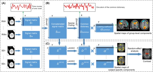
The process for the group spatial sparse representation (group‐SSR) model. (A) The fMRI signals for an individual subject in the RW or SD condition are extracted and expressed as a data matrix S _i after the preprocessing and normalization steps. Each column in S _i represents the time course at one single voxel. (B) All fMRI data matrices are temporally concatenated into a large data matrix S _con, in which each column contains a concatenated time course. Then, a group‐level dictionary D _common is learned to extract k dictionary atoms with the corresponding sparse loading coefficients α _common by solving an LASSO problem. Each row in α _common is the sparse spatial map of the corresponding atom of D _common within the whole brain, and each column presents the sparse weights of atoms of D _common when interpreting the corresponding voxel's fMRI signal. (C) The common dictionary is split into (m + n) subsets for each scan. Then, on the basis of D ⁽ⁱ⁾, the subject‐specific loading coefficients α ⁽ⁱ⁾ are obtained from the individual data matrix S ⁽ⁱ⁾ by resolving an LASSO problem. Each row in α ⁽ⁱ⁾ is the subject‐specific spatial map of the corresponding atom of D ⁽ⁱ⁾ within the whole brain. Consequently, a random effect analysis can be conducted on the specific spatial maps to evaluate the significance of spatial mappings or compare the expression differences of the atoms between the RW and SD conditions. [Color figure can be viewed at http://wileyonlinelibrary.com]

Next, all fMRI data matrices from each subject were temporally concatenated into a large data matrix $S_{\mathrm{con}}={[S_1,\hspace{0.17em}\dots ,\hspace{0.17em}{S}_m,\hspace{0.17em}{S}_1,\hspace{0.17em}\dots ,\hspace{0.17em}{S}_n]}^T\in R^{(m+n)t\times k}$, in which each column contains a concatenated time course. Then, using an effective online dictionary learning algorithm [Mairal et al., 2014], a common dictionary $D_{\text{common}}\in R^{(m+n)t\times k}$, containing k atoms was learned to represent the concatenated data matrix $S_{\text{con}}$ with the corresponding common sparse loading coefficients ${\alpha }_{\text{common}}\in R^{k\times v}$ as follows:

$$S_{\text{con}}=D_{\text{common}}\times {\alpha }_{\text{common}}$$ (2)

Each row in ${\alpha }_{\text{common}}$ is the sparse spatial map of the corresponding common atom, and computing the row norms of the ${\alpha }_{\text{common}}$ allowed us to rank the atoms with respect to their importance for decomposition. Each column of ${\alpha }_{\text{common}}$ presents the sparse weights of atoms in $D_{\text{common}}$ when interpreting the corresponding voxel's fMRI signal (Fig. 1B). The amplitude of each weight reflects the contribution of each voxel to distributed and coherent activity within that atom (i.e., functional connectivity).

In fact, the sparse representation procedure [Eq. (2)] aims to solve an L1‐regularized LASSO problem [Yeo et al., 2011]:

$$\underset{D\in R^{t\times k},\alpha \in R^{k\times v}}{\min }\frac{1}{2}{\Vert S-D\alpha \Vert }_2^2+\lambda {\Vert \alpha \Vert }_1$$ (3)

where S is the whole‐brain fMRI signal matrix, D is the learned dictionary, $\alpha$ is the corresponding loading coefficients, and $\lambda$ is the parameter for a regression residual and sparsity level tradeoff. In addition, each atom of D is constrained by Eq. (3) to avoid a trivial solution of the optimization.

$$C\stackrel{\Delta }{=}\{D\in R^{t\times v},s.t.\hspace{0.17em}\forall j=1,\hspace{0.17em}\dots ,\hspace{0.17em}k,\hspace{0.17em}{d}_j^T{d}_j\le 1\}$$ (4)

We used a fast implementation in the optimization MATLAB toolbox SPAMS (SPArse Modeling Software, http://spams-devel.gforge.inria.fr/) to find the optimal solution in Eq. (3) by alternately updating either of matrix $D$ or $\alpha$, while the other was held fixed [Mairal et al., 2009]. For each atom, we used 1000 bootstrapping tests with resampling and data replacement to eliminate the influence of noise and interindividual variability to obtain the comparatively reliable group maps. Labeling of the atoms from each run of bootstrapping was performed based on their spatial overlap with the atoms from the full sample. That is, a particular “atom 1” was assigned the same label as the atom from the full sample with the maximal spatial overlap. For each atom, the bootstrap ratio, a normalized measure of the reliability of the weight salience, was calculated by dividing the bootstrap mean salience of each weight by its standard error [Qin et al., 2015]. Finally, weights with a bootstrap ratio value within a certain range (approximately 99% confidence interval) were selected as salient loading coefficients of the atom.

Parameter Selection

In this model, the dictionary size k and the sparsity level $\lambda$ are free parameters. The values of k and $\lambda$ directly determine how well the model fits the observed data. In particular, as k is increased or $\lambda$ is reduced, the approximation error is reduced. However, this may result in overfitting beyond a certain value of k or $\lambda$. Here, a grid search procedure based on the measure of the Akaike Information Criterion (AIC) was applied to parameter selection. For each pair of k and $\lambda$, an approximation error was calculated with Eq. (5).

$$\text{Rss}={\displaystyle \sum _{i=1}^N{(S^{(i)}-D^{(i)}{\alpha }^{(i)})}^2}$$ (5)

where $N=m+n$ is the number of all scans. In addition, AIC was defined as follows:

$$\text{AIC}=2K+N\cdot \text{In}(\text{Rss}/N)$$ (6)

where the number K of model parameters was set to be $K=k+1$ for each fixed $\lambda$, when any least squares model [Eq. (5)] with independently and identically distributed (i.i.d.) Gaussian residuals was assumed [Burnham et al., 2004]. The values of k and $\lambda$ corresponding to the point where AIC reaches a minimum are preferred for model building.

Reproducibility Estimation

The bootstrapping procedure was adopted to assess the accuracy and reproducibility of the group sparse spatial patterns of the atoms. For each bootstrapping run, a common dictionary containing k atoms with the corresponding spatial maps was learned to represent the concatenated fMRI signals from the selected samples. In addition, the eta² was applied to estimate the similarity of two spatial maps [Lei et al., 2016].

$${\text{eta}}^2=1-\frac{{\text{SS}}_{\text{Within}}}{{\text{SS}}_{\text{Total}}}=1-\frac{{\sum }_{i=1}^v[{(a_i-m_i)}^2+{(b_i-m_i)}^2]}{{\sum }_{i=1}^v[{(a_i-\overline{M})}^2+{(b_i-\overline{M})}^2]}$$ (7)

where a_i and b_i are the values in position i of matrix a and matrix b, m_i is the mean of a_i and b_i, and $\overline{M}$ is the grand mean value across all positions in the two matrices.

To further evaluate the reproducibility of the spatial patterns across different datasets, we used another publicly available dataset from the Neuroimaging Informatics Tools and Resources Clearinghouse (NITRC) website, contributed by the Centers of Biomedical Research Excellence (COBRE; http://fcon_1000.projects.nitrc.org/indi/retro/cobre.html). We randomly selected 60 healthy subjects as the alternate dataset (TR = 2000 ms). The same process was used for all preprocessed scans, and subsequently, the sparse learning algorithm depicted in Figure 1 was also run on this dataset.

Random Effect Analysis

The learned common dictionary from Eq. (2) represents the common temporal components of fMRI data for all subjects, which can be split into (m + n) subsets for each subject. Thus, Eq. (1) can be rewritten as Eq. (8):

$$\left[\begin{array}{c}{S}^{(1)}\\ ⋮\\ S^{(m+n)}\end{array}\right]=\left[\begin{array}{c}{D}^{(1)}\\ ⋮\\ D^{(m+n)}\end{array}\right]\times {\alpha }_{\text{common}}$$ (8)

where $S^{(i)}$ represents the fMRI data of the i‐th subject and $D^{(i)}$ is the subset of the population dictionary responding to the i‐th subject. Thus, for the subject i, the subject‐specific loading coefficients ${\alpha }^{(i)}\in R^{k\times v}$ can be obtained by resolving an L1‐regularized LASSO problem for the sparse representation of S ^{( i )}:

$$\underset{{\alpha }^{(i)}\in \hspace{0.17em}{R}^{k\times v}}{\min }\frac{1}{2}{\Vert S^{(i)}-D^{(i)}\Vert }_2^2+\lambda {\Vert {\alpha }^{(i)}\Vert }_1$$ (9)

This would produce the projection of individual data S ^{( i )} on the group dictionary estimation of D; that is, the individual data S ^{( i )} can be reconstructed with the subject‐specific loading coefficients ${\alpha }^{(i)}$:

$$S^{(i)}=D^{(i)}\times {\alpha }^{(i)}$$ (10)

For the i‐th subject, the k‐throw in ${\alpha }^{(i)}$ represents the reconstructed subject‐specific weights corresponding to the k‐th atom of population dictionary $D$, which leads to sparsely distributed spatial mapping (Fig. 1C) specific to this subject. For all subjects, we calculated the mean and variance of each spatial mapping across subjects, where the variance across subjects was used as an estimate of the population variance. A hypothesis test was then used to provide a “random effects” inference. That is, the weights of voxels within a set of sparse dictionary atoms were treated as random variables, and a one‐sample t test with the null hypothesis of zero weights or a two‐sample t test for comparison between conditions (e.g., RW and SD stages in this study) was performed.

Comparison with Group Spatial ICA

We evaluated the performance of the group‐SSR model by comparing the results with the group ICA. Group spatial ICA was conducted on the 35 RW scans using the GIFT software (http://icatb.sourceforge.net/) [Calhoun et al., 2001, 2009] with the same component number of k . A standard procedure in GIFT processing was performed, including dimension reduction with PCA, ICA decomposition based on temporally concatenated data for all subjects, and a back‐reconstruction step for subject‐specific spatial maps of components. Finally, a one‐sample t test (P < 0.05, FWE corrected) was performed to make group‐level random‐effects inferences based on the subject‐specific spatial maps. The obtained ICA inferences were further compared with the common dictionary atoms derived from the group‐SSR algorithm.

The spatial overlap rate (SOR) was defined to quantitatively measure the extent to which the components overlapped [Lv et al., 2015b]:

$$SO{R}_i=\frac{R_i}{R_{\text{involved}}}\times 100\%$$ (11)

where the subscript i represents the number of overlap components in group‐SSR or group‐ICA. $R_i$ is the number of voxels simultaneously belonging to i components and $R_{\text{involved}}$ represents the number of voxels involved in at least one component. Finally, we evaluated the ability of group‐SSR to extract the overlap patterns by comparing the SORs between group‐SSR and group‐ICA.

A significant virtue of ICA is that it allows the detection of random noise and confounding signals such as pulsation and breathing artifacts, thereby providing an effective tool for denoising fMRI [Mckeown et al., 2003]. Here, we used a relatively high model order (number of atoms, k = 100) to investigate whether the proposed model can effectively identify atoms representing physiological, movement‐related, or imaging artifacts. Analysis was performed on the data concatenated with preprocessed fMRI signals from all voxels within the whole brain from the 35 RW scans but without band‐pass filtering to facilitate the investigation of the spectral distributions of each atom. Each atom was visually inspected to separate artifacts from meaningful functional networks according to its spatial distribution, as signal atoms should exhibit peak activations in gray matter, while noise atoms can have spatial overlap with white matter and/or cerebrospinal fluid or may be located at the edges of the brain [Allen et al., 2011; Griffanti et al., 2014]. As previous studies have suggested that meaningful resting‐state networks have differentiated spectral distributions from physiological components [Allen et al., 2011; Robinson et al., 2009], we also evaluated the spectral distributions of atoms with the expectation that predominantly low‐frequency (<0.1 Hz) power spectra will be found for the atoms corresponding to ICNs. Specifically, the ratio of the integral of spectral power below 0.10 Hz to the integral of power between 0.15 and 0.25 Hz that has been applied as a quantitative indicator in ICA‐based noise‐component identification [Allen et al., 2011] was used to differentiate the artifact atoms and the ICN atoms.

Previous ICA‐based decomposition analyses have demonstrated that removal of the time series of noise components out of the signals of the ICN components effectively improves the sensitivity of ICN detection [Griffanti et al., 2014]. Similarly, we investigated whether a similar cleaning procedure in the group‐SSR model improves identification of the ICNs. The cleanup was performed by regressing the time series corresponding to the group‐level artefact atoms from those corresponding to the nonartefact atoms (signal atoms) derived from the concatenated dataset. The group spatial maps were obtained via a one‐sample t test on the subject‐specific spatial maps for each nonartefact atom. The effect of noise cleaning was further evaluated by comparing the temporal power spectra and the group spatial maps of the uncleaned atoms with those of the cleaned atoms.

RESULTS

Grid Search for Parameter Selection

Although there are no golden criteria for defining the sparsity λ, previous studies regarding the sparse decomposition of fMRI signals have suggested a sparsity of 0.1–1 provided a good tradeoff between the involved noise and the sparse level of atoms [Lv et al., 2015a; Zhang et al., 2015]. Hence, a grid search procedure with $\lambda$ from 0.1 to 0.5 and $k$ from 8 to 40 was used to determine the optimal model parameters herein. For each pair of $k$ and $\lambda$, the group‐SSR model was applied to the entire data set from the 35 RW and 26 SD scans. The variation of AIC with the change of $k$ and $\lambda$ is shown in Figure 2. The AIC tended to decrease with a decrease in $\lambda$. The minimum of the AIC curves corresponding to the values of $k=20$ and $\lambda =0.1$ as a tradeoff between model complexity and risk of overfit was chosen to build the model.

Figure 2.

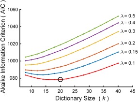
Grid search results for parameter selection. The point corresponding to the value of k = 20 and λ = 0.1 was selected for model building. [Color figure can be viewed at http://wileyonlinelibrary.com]

Spatial Maps of Group‐Level Atoms

Next, we investigated whether the proposed method can identify the resting‐state functional networks in normal subjects. Thus, only the 35 RW scans were used in the group‐SSR model depicted in Eq. (2) with the parameters $k=20$ and $\lambda =0.1$. Consequently, a common dictionary containing twenty atoms was learned to represent the concatenated data matrix with the corresponding sparse loading maps. For each atom, the corresponding loading coefficient at an individual voxel reflects the extent to which this voxel is involved in this atom. Due to noise and individual variability, only those weights with a bootstrap ratio value above 16 or below −16 (responding to the 99% confidence interval, slightly different for each atom) were selected as the salient weights (Fig. 3). These sparse weights, which are shown in Figure 4, depict the cortical distribution (maps) of the corresponding atom. Furthermore, each of the spatial maps consists of multiple specific regions. Importantly, we observed that some specific regions, such as the inferior parietal lobule (IPL), precuneus and thalamus, are involved in multiple atoms (see Fig. S1 in Supporting Information), which have been identified by previous studies as functional or structural hubs in the brain [Hallquist et al., 2013; Wang et al., 2012].

Figure 3.

Demonstration of the selection of the sparse weights' threshold. For each atom, the weights with a bootstrap ratio value above 16 or below −16 (approximately 99% confidence interval, slightly different for each atom) were selected as salient loading coefficients of the atom. [Color figure can be viewed at http://wileyonlinelibrary.com]

Figure 4.

Spatial maps represented by loading weights of the learned common dictionary for the RW group. [Color figure can be viewed at http://wileyonlinelibrary.com]

To demonstrate the functional brain networks that these atoms are assigned to, we summarized the proportions of the voxels that fall within each of the seven cortical networks previously reported [Yeo et al., 2011] within an individual atom. These networks include the default mode, dorsal and ventral attention, frontoparietal, limbic, somatomotor, and visual network. The overlapping rates of these atoms with the seven cortical networks are shown in Figure 5.

Figure 5.

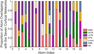
The proportion of the 20 group‐level atoms overlapping with the seven cortical networks. DMN, default mode network; dATN, dorsal attention network; vATN, ventral attention network; FPN, frontoparietal network; Limbic, limbic network; SMN, somatomotor network; VN, visual network. [Color figure can be viewed at http://wileyonlinelibrary.com]

Figure 5 indicates that some atoms are predominantly involved in a single cortical network. For example, atoms 5, 6, 8, and 15 are primarily related to the visual network, while a large part of atom 10 is involved in the frontoparietal network. Atoms 7and 13 mainly consist of portions of the default‐mode network, and atoms 12 and 19 are primarily associated with the somatomotor network and the dorsal attention network, respectively.

In addition, some of the other atoms are believed to simultaneously cover multiple functional networks without a prominent proportion overlapping on any single network. For example, atom 1 covers the default‐mode network, frontoparietal network, and somatomotor network. Atom2 is involved in the dorsal attention network and visual network, while atom 18 covers the default‐mode, dorsal and ventral attention, and frontoparietal networks. In particular, atom 11 is associated with six cortical networks but not the frontoparietal network.

Reproducibility

The reproducibility of the atoms was assessed with a 1000‐bootstrapping resampling procedure. For each run during bootstrapping, the same parameters and model were performed on the resampled data, which consequently resulted in 1000 corresponding spatial maps for each atom. The spatial correlation coefficients as similarity measures between these spatial maps and the spatial map obtained from all 35 RW scans are summarized and shown in Figure 6A. For each atom, high spatial similarities across the loading maps obtained from different bootstrapping runs were observed (with a mean similarity value of 0.85).

Figure 6.

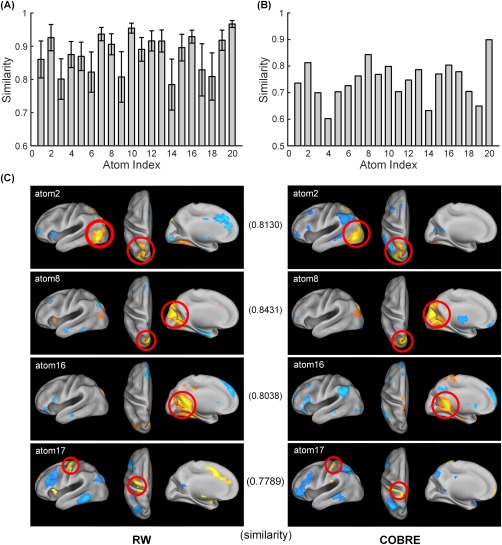
The reproducible results of the group sparse spatial patterns of the 20 atoms. (A) The reproducibility of the atoms was assessed with a 1000‐bootstrapping resampling approach. The error bar represents the mean and standard deviation of the spatial similarities of the loading weights obtained from different bootstrapping runs. It is evident that these weight maps across bootstrapping runs exhibit high spatial similarities. (B) The reproducibility of the atoms was estimated using the publicly available COBRE dataset, where the spatial maps of atoms were reasonably reproduced. (C) Pairwise comparison of the four atoms computed from the RW scans (left) and COBRE (right). The inner product value for each comparison reflects the high spatial similarity between the paired atoms.

To further estimate the reproducibility of our results across datasets, the group‐SSR model was also applied to an alternate cohort that consisted of 60 healthy samples randomly selected from the publicly available COBRE dataset. We observed that the spatial maps of atoms were reasonably reproduced in the COBRE dataset with an average similarity value of 0.75 (Fig. 6B). Additionally, a side‐by‐side comparison of four atoms computed from the RW scans and the COBRE dataset is shown in Figure 6C.

Alteration of Functional Networks Following Sleep Deprivation

We further inspected the changes in the expression of each atom following SD. First, group‐SSR was applied to the concatenated matrix of qualified acquisition data from the RW and SD scans of 26 subjects to obtain the group reference and the individual loading weights. A random effect analysis of a paired‐sample t test was then performed to test the significance of between‐group differences in the subject‐specific loading map. We found significant contribution differences in 5 out of the 20 atoms (SD vs RW, paired‐sample t test, P < 0.01, FDR‐corrected) shown in Figure 7. These altered brain regions with their cluster sizes, peak coordinates, and maximum t values of statistical significance are detailed in Table 1.

Figure 7.

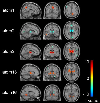
Five atoms exhibited significant changes in the loading weights between the SD and RW conditions with global signal regression (SD vs RW, paired‐sample t test, P < 0.01, FDR‐corrected). [Color figure can be viewed at http://wileyonlinelibrary.com]

Table 1.

The specific brain regions, cluster size, peak coordinates, and maximum t value of significant weight differences of atoms between the SD and RW conditions with global signal regression (SD vs RW, paired‐sample t test, P < 0.01, FDR‐corrected)

	Regions (AAL)	Cluster size	Peak coordinates			t value
			x	y	z
atom1	Precuneus_R	92	9	−55	42	8.2656
	Temporal_Mid_R	41	54	−15	−24	4.9375
	Frontal_Inf_Tri_L	264	−54	12	21	−7.8256
	Frontal_Inf_Oper_L
	Frontal_Mid_L
	Precentral_L
atom2	Thalamus_R	283	3	−18	3	−9.5534
	Thalamus_L
	Temporal_Mid_L	47	−54	−6	−21	5.1311
	Calcarine_R	118	6	−90	6	−6.5417
	Cingulum_Ant_L	180	0	36	9	−7.2538
	Cingulum_Ant_R
atom3	Vermis_9	40	3	−60	−39	5.9226
	Vermis_8
	Thalamus_L	526	12	−12	3	8.7746
	Thalamus_R
	Putamen_L
	Putamen_R
	Pallidum_L
	Pallidum_R
	Precuneus_R	41	9	−69	42	−5.3961
	Temporal_Mid_R	95	54	−57	9	−5.7268
atom13	Amygdala_L	25	−27	−3	−12	6.7053
	Hippocampus_L
	Thalamus_L	196	−15	−15	9	6.1457
	Putamen_L
	Pallidum_L
	Putamen_R	82	30	−6	−12	5.7567
	Pallidum_R
	Amygdala_R
	Precentral_L	50	−33	−21	51	−5.6978
	Postcentral_L
	Precuneus_R	66	9	−57	15	−6.3185
	Thalamus_R	69	12	−18	12	5.2317
atom16	Lingual_L	55	−15	−51	−9	6.023
	Cerebelum_4_5_L
	Precuneus_R	68	18	−54	18	−6.9953
	Calcarine_R
	Lingual_R	56	24	−54	−9	5.6273
	Cuneus_R	24	6	−84	33	6.1145

A significant decrease in functional connectivity within some distributed regions, including the bilateral thalamus, right calcarine, and bilateral anterior cingulate cortex, was observed in atom 2. By contrast, atom 13 identified widespread regions with increased contribution, mainly located in emotion or memory systems, such as the bilateral amygdala, putamen, pallidum, thalamus, and left hippocampus. Other atoms exhibited more complex functional alterations caused by SD. Atom3, for example, showed increased contribution of the cerebellum, bilateral thalamus, putamen, and pallidum but decreased contribution in the right middle temporal gyrus. Similarly, increased contribution of the right precuneus and right middle temporal gyrus along with decreased contribution of the left frontal cortex and precentral was found in atom 1. In atom16, increased contribution was found in the bilateral lingual gyrus, right cuneus, and the left cerebellum, along with decreased contribution in the right calcarine and the right precuneus.

As we expected, some regions, such as the thalamus, which participates in multiple atoms, exhibited distinct response patterns across different atoms. For atom 2, the thalamus showed a significantly decreased contribution. In atoms 3 and 13, however, we observed an obvious increase in functional connectivity of the bilateral thalamus. Another example is the right precuneus, which exhibited a stronger contribution in atom 1 but a reduced contribution in atom 16 (Table 1).

As shown in Figure 8A, we see that the bilateral default mode areas represented by atom 7 are significantly anticorrelated with the dorsal attention systems represented by atom 19.This anticorrelation between task‐positive regions and a task‐negative system is a well‐known finding in previous literature [Mairal et al., 2009]. Of greater interest is that this anticorrelation tended to be weakened after SD in contrast to the RW condition (Fig. 8B; RW/mean = −0.17, std = 0.19; SD/mean = −0.05, std = 0.17; paired‐sample t test, P = 0.0186). To further illustrate this change, Figure 8C depicts the time course for atoms 7 and 19 for a selected subject, and their alteration in anticorrelation between the SD and RW conditions.

Figure 8.

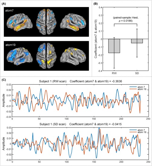
SD decreased the anticorrelation between the default mode network and dorsal attention network represented by atoms 7 and 19, respectively. (A) Cortical maps of atoms 7 and 19. (B) The paired‐sample t test result revealed a significant decrease in the anticorrelation between the two atoms in the SD condition compared with the RW condition. (C) The correlation coefficients between atoms 7 and 19 for an exemplar subject, along with the associated atom time courses. [Color figure can be viewed at http://wileyonlinelibrary.com]

Impact of Global Signal Regression (GSR)

To evaluate the impact of GSR on our results, we reran the sparse dictionary learning and statistical analysis without GSR, which revealed that the GSR preprocessing step induced substantial changes.

The global signals impacted the BOLD contrast between the RW and SD conditions in two aspects (compare Fig. 7 with Supporting Information, Fig. S2 and refer to Table 1 and Supporting Information, Table S1 for details). First, due to the increase in the global signals, the decline in the expression of the atoms in some regions was significantly weakened, and more regions with increased contribution were observed within some of these atoms. As an example, atom 2 included more widespread regions associated with attention or alertness processing that showed increased functional connectivity during SD (compare the Table 1 and Supporting Information, Table S1). Moreover, the anterior cingulate was no longer significantly different due to the influence of the global signals. Second, the global signals produced more atoms exhibiting significant differences. For example, atom 7 showed significantly decreased expression in the cerebellum and thalamus.

Comparison with Group‐ICA

Twenty group‐level spatial independent components of the 35 RW scans were obtained using the group‐ICA approach. One component was identified as the default mode network (DMN) based on its maximal spatially overlapping rate with the DMN template [Yeo et al., 2011]. Among the dictionary atoms, atoms 7 and 13 dominantly participated in the DMN, as shown and compared to the ICA‐derived DMN component in Figure 9. Note that more brain regions were observed in the two DMN atoms than in the group‐ICA‐based DMN component. These additional regions included task‐positive areas that demonstrated a clear negative correlation with the DMN areas.

Figure 9.

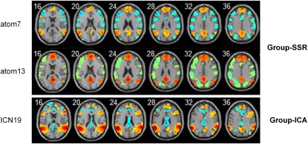
Comparison of the DMN components obtained from group‐SSR and group‐ICA. Atoms 7 and 13 showed separate parts of the DMN, suggesting a differential contribution of these DMN regions within these atoms. Moreover, compared with the DMN component from group‐ICA, these atoms involve more anticorrelated areas with the DMN (one‐sample t test, P < 0.05, FWE corrected). [Color figure can be viewed at http://wileyonlinelibrary.com]

We also compared the thalamus‐related components between group‐SSR and group‐ICA. In the group‐SSR model, the thalamus was observed to be involved in three sparse atoms, including atoms 4, 14, and 17, in contrast to a single component associated with the thalamus in the group‐ICA model (Fig. 10A).

Figure 10.

(A) The components involving the thalamus were extracted from group‐SSR and group‐ICA. The thalamus was found to participate in multiple functional networks through the group‐SSR. (B) Comparison of the spatial overlap rates (SORs) of the components in the group‐SSR and the group‐ICA models (one‐sample t test, P < 0.05, FWE corrected). [Color figure can be viewed at http://wileyonlinelibrary.com]

Furthermore, Figure 10B presents the comparison between the spatial overlap rates (SORs) of the components derived from the group‐SSR and group‐ICA models. Notably, both models identified the overlap networks underlying the rs‐fMRI data. However, group‐SSR showed relatively higher SORs than group‐ICA when the number of overlap components was > 3.

Identification of Noise Atoms

In the group‐SSR segment with a high model order (k = 100), 30 atoms were manually identified as noise atoms and 42 atoms were identified as signal atoms based on their spatial distribution. The remaining 28 atoms were identified as mixed atoms, representing a mixture of ICNs and artefact sources. These mixed atoms showed significant expression in both gray matter and white matter and/or cerebrospinal fluid, and hence are not able to fully represent noise or signal. The spatial distribution and frequency spectra of three atoms are shown in Figure 11A as exemplars of the three atom types found. Figure 11B plots the media frequency spectra of the signal, mixed, and noise atoms averaged over subjects. Furthermore, the ratios of low‐frequency (LF) to high‐frequency (HF) power for each atom were calculated and statistically compared between the three groups. Both the signal atoms and the mixed atoms had significantly higher ratios of LF to HF power than the noise atoms at a group level (Fig. 11C, two‐sample t test, P < 0.01), while no significant difference in the LF to HF ratio was found between the signal atoms and the mixed atoms.

Figure 11.

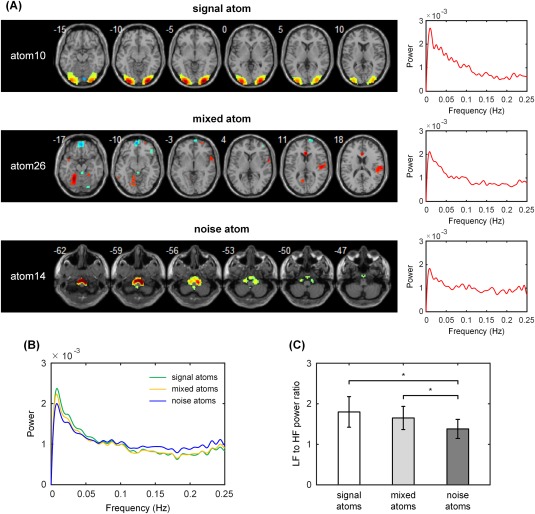
The ability of the group‐SSR model to identify noise components was investigated using a relatively high model order (number of atoms, k = 100). (A) The spatial distribution and frequency spectra of three atoms are shown as exemplars of signal, mixed and noise atoms, respectively. (B) The median frequency spectra of the signal, mixed and noise atoms averaged over subjects. (C) The ratios of low frequency (LF) to high frequency (HF) power for the atoms. Both the signal atoms and the mixed atoms had significantly higher ratios of LF to HF power than the noise atoms at a group level, while no significant difference was found between the signal atoms and the mixed atoms. *Two‐sample t test, P < 0.01. [Color figure can be viewed at http://wileyonlinelibrary.com]

After cleaning up the signal atoms by regressing the time series corresponding to the noise atoms, the group spatial maps of the cleaned signal atoms were relatively more concentrated compared with the uncleaned atoms (Supporting Information, Fig. S3A). Furthermore, this cleanup resulted in an apparent decrease in power of the signal atoms both at LF and HF (Supporting Information, Fig. S3B). Meanwhile, the cleaned signal atoms exhibited significantly higher ratios of LF to HF power in contrast to the uncleaned atoms (see Supporting Information, Fig. S3C for detail). These results demonstrated the potential of the group‐SSR model to better identify ICNs following the noise‐cleaning procedure.

DISCUSSION

We have demonstrated that multiple resting‐state functional brain networks can effectively be identified based on a group‐level sparse representation of rs‐fMRI data by permitting their spatial overlap. By splitting the resulting dictionary atoms into individual‐specific components, we have obtained common temporal components represented by the atoms within the population and subject‐specific spatial maps of these atoms, which can facilitate subsequent group random effect analysis. We further validated the feasibility of this approach by applying it to identify changes in resting‐state functional networks during SD. Finally, we successfully extracted multiple cognitive brain networks linked to SD. Notably, the thalamus was observed to participate in multiple functional networks and exhibited distinct response patterns within these functional networks. These results indicate that our models for making group inference scan provide new insights into the functional architecture of the brain by permitting spatial overlap between functional brain networks and can facilitate the description of the varied relationships of the overlapping regions with other regions of the brain in the context of different functional systems.

Group Inference for RW Scans

As the RW data show (Fig. 4), this approach is able to identify multiple functional patterns that consist of functionally coherent or anti‐correlated regions in a data‐driven manner without any prior knowledge of a seed region of interest. Compared with the spatial ICA, an advantage of dictionary learning of fMRI signals is its greater potential for identifying positive and negative correlations within the same atoms [Eavani et al., 2015]. For example, atoms 7 and 13 clearly represent the lateral and medial part of the DMN, respectively. These atoms fit well with the independent component 19 from the group ICA analysis but suggest a differential contribution of these DMN regions within these atoms (Fig. 9). Of greater interest are additional brain regions in the DMN atoms that include other network components such as task‐related or anti‐task‐related components. These regions are not necessarily spatially independent and, consequently, have not been detected via the ICA, which assumes spatial independence of the network components.

The coverage of multiple functional systems by most of the atoms likely reflects subtle functional interaction across networks. In the group‐SSR model, atoms are defined by temporal coherence in LF fluctuations, without constraints of spatial independence across components. Given that the time course of one region can be represented by a linear mixture of multiple temporal components, this approach intrinsically provides decomposes signals at a single region into multiple components that are likely to be assigned to different atoms. This rationale leads to greater distribution of coherent regions in an individual atom and highlights the diversity of the functional roles of the overlapping regions in different functional brain systems. This strategy is in accordance with current viewpoints on the principles of functional organization in the brain. For example, many association regions appear to participate in multiple networks, and integration of networks in the association cortex has been suggested to be a true feature of cortical organization in the brain [Yeo et al., 2014]. The degree of integration of even some multiple‐network hub regions into different networks varies dynamically over time [Schaefer et al., 2014]. In addition to this functional evidence, histological and electrophysiological studies have suggested that functional heterogeneity of intermixed cortical neurons within the same region is a general property of the cortex [Xu et al., 2016]. A plausible explanation is that a typical fMRI voxel contains at least hundreds of thousands of neurons that receive inputs from and send outputs to extensive cortical and subcortical areas. Hence, the BOLD signals from an individual voxel reflect a highly heterogeneous mixture of functional activity associated with different neural circuits. Thus, our approach provides a more flexible model to disentangle the heterogeneous components of BOLD signals from a single voxel, facilitating the description of multiple functional roles of the same cortical region.

The reproducibility of the identified sparse spatial patterns was evaluated within the same dataset and across datasets. Notably, the atoms from different datasets (Fig. 6B) had lower similarity compared to the bootstrapping runs of the same dataset (Fig. 6A). The decline in the stability of the atoms across datasets is likely due to the effect of site, since significant and quantitatively important inter‐site differences in the temporal signal‐to‐noise ratio of resting‐state fMRI data have been associated with hardware and pulse sequence differences across scanners [Jovicich et al., 2016].

Alteration of Multiple Functional Networks Following Sleep Deprivation

Utilizing a paired‐sample t test statistics method based on the group inferences, we demonstrated multiple alterations in functional brain circuits following SD, particularly in the dorsal attention, default mode, visual, frontal, auditory, motor, auditory/speech, amygdala/hippocampal, and cerebellar networks, in line with previous findings [Kaufmann et al., 2016; Yeo et al., 2015]. For example, atom 2 exhibited a significant decrease in functional connectivity in the bilateral thalamus, bilateral anterior cingulate cortex (ACC) and right calcarine. Non‐GSR (without global signal regression) results further showed increased contributions of widespread regions including the angular gyrus, left middle temporal, lingual, postcentral, and frontal cortex, along with the increase in the thalamus (Supporting Information, Table S1). Most of these regions belong to the frontoparietal control and attention networks, which have been reported to change during SD [Kaufmann et al., 2016]. For example, an early PET study found a predominant decrease in the regional cerebral metabolic rate in the thalamus during SD, and a decline in alertness and cognitive performance associated with thalamus deactivation [Thomas et al., 2003]. Recent fMRI studies also revealed hypoactivation in the inferior parietal regions after SD, which was linked to a decrease in attentional resources. Compensatory increases in the prefrontal cortex and parietal lobe during SD have also been observed during task performance, suggesting that sleep‐deprived individuals require more attentional resources to sustain normal attentional vigilance [Drummond et al., 2005, 2001]. Additionally, the increased activation of the temporal, frontal, and visual cortexes is compatible with the recent reports regarding decreased anticorrelation between the DAN and DMN and a stronger interaction effect of the visual‐DMN [Havas et al., 2012; Kaufmann et al., 2016; Yeo et al., 2015], although the increased expression in these regions was mainly attributed to the promotion of global activity after SD (refer to Supporting Information, Table S1).

Furthermore, atom 13 exhibited significantly increased expression in the left hippocampus, bilateral thalamus, bilateral amygdala, and bilateral putamen, extending recent findings of weaker functional connectivity between the hippocampus and the DMN [Yeo et al., 2015], stronger functional connectivity between the amygdala and left posterior cingulate cortex/precuneus [Shao et al., 2014], and decreased activity within the DMN [Havas et al., 2012] during SD. These results align with recent findings of impaired memory and emotion processing following short‐term SD [Chee et al., 2006; Gujar et al., 2011; Yoo et al., 2007]. We also observed significant changes in the visual cortex in atom 16, including the left lingual and rightcalcarine. Meanwhile, as the key node of the posterior DMN, the right precuneus showed a decreased contribution, as supported by recent evidence of changes in visual‐DMN functional connectivity during SD [Kaufmann et al., 2016; Yeo et al., 2015]. Notably, atom 3 showed increased expression in the bilateral thalamus and decreased expression in the middle temporal gyrus, implying an impairment in auditory processing caused by SD [Liberalesso et al., 2012].

We also replicated the previous finding of decreased anticorrelation between the DMN and dorsal attention network (DAN) [Havas et al., 2012; Kaufmann et al., 2016; Yeo et al., 2015], with the results shown in Figure 8. As shown in Figure 8A, atoms 7 and 19 identify the DMN and the DAN (extending to the frontoparietal network), respectively. We observed a strong anticorrelation between the time courses of the two atoms that decreased after SD (paired‐sample t test, P < 0.05). This weaker anticorrelation between the DMN and DAN has been linked to a decline in attentional vigilance during SD, which is compatible with the ability of the anticorrelation strength between the DMN and DAN to predict the vulnerability to vigilance decline following SD [Yeo et al., 2015].

Notably, the aforementioned results were obtained by regressing out the global signals from each individual's data. According to a study concerning the impact of the global fMRI signal on SD, GSR may be beneficial in certain experimental contexts [Yeo et al., 2015]. Previous studies also demonstrated that GSR facilitates the delineation of functional systems by removing the confounding effects of head motion and other non‐neuronal sources of noise [Satterthwaite et al., 2012]. Moreover, GSR can enhance the overall neuronal‐hemodynamic correspondence [Keller et al., 2013] and affords increased tissue sensitivity [Fox et al., 2009] and decreased dependencies on motion [Saad et al., 2013]. However, it has been argued that the global signals have a potential neural basis. For example, global signals have been reported to be related to neural activity in anesthetized monkeys and highly correlated with gray matter signals [Fox et al., 2009; Yan et al., 2013].In particular, a significant increase in the global signals during SD has been observed, and increased amplitude of this signal is related to the decreased vigilance after SD [Thompson et al., 2013; Wong et al., 2013].

The global signals led to more atoms exhibiting significant differences, some of which were supported by previous findings regarding SD. For example, the significantly decreased contribution of the cerebellum and thalamus in atom 7 (Supporting Information, Fig. S2) is in line with the evidence of reductions in absolute regional cerebral metabolic rate for glucose in the temporal lobes, thalamus, and cerebellum after short‐term SD [Thomas et al., 2003; Wu et al., 1991] and decreased protein levels in the cerebellum after selective REM SD in rats [Sei et al., 2000]. Atom 17 exhibited altered expression in some nodes of the salience and vigilance networks, including the bilateral precuneus and medial superior frontal cortex. Additionally, the alteration of signals in the posterior and middle cingulate cortex are supported by the recent evidence that SD decreases the functional connectivity between the posterior and anterior cingulate cortex [Bosch et al., 2013) and impairs the effective connectivity from the posterior to anterior cingulate regions, proportional to its deleterious effect on vigilance [Piantoni et al., 2013].

The significant differences between the results with GSR and without GSR can be explained by a recent suggestion that some of the statistical differences between RW and SD are attributable to the increase in whole‐brain signals after SD, while others are due to the changes in fluctuations of fMRI signals relative to the whole‐brain fMRI signals calculated by GSR [Yeo et al., 2015]. We also note that the contrast within some regions (e.g., the thalamus in atom 2 and the lingual gyrus in atom 16) became more significant when the whole‐brain signal was regressed. This is in accordance with recent results on the prediction of vulnerability to SD indicating that resilient and vulnerable subjects can be more strongly differentiated when relative fluctuations of the whole‐brain signal are considered [Yeo et al., 2015]. Obviously, our approach works well for identifying the effects of global signals on the changes in the brain following SD.

Methodology Consideration

The group‐SSR approach used here identifies group inferences assuming temporal common spatial maps for all subjects but allowing for overlap among inferences. While this approach may resemble the group spatial ICA implemented in GIFT software (http://icatb.source-forge.net/) [Calhoun et al., 2001], there are several important differences. First, the spatial ICA identifies spatially distributed but temporally coherent brain regions as functional networks by explicitly assuming the independence of fMRI signals across the components while the group‐SSR approach does not. As indicated in recent studies, fMRI signals are not necessarily independent [Daubechies et al., 2009]. Coincident with this viewpoint, the proposed approach assumes that the fMRI signals of each voxel of each subject are sparsely represented by a linear combination of those signals of the functioning network components. Hence, our model offers a novel, alternative method to examine the spatial organization of cortical function based on the interaction of multiple concurrent neural processes or networks. Second, group‐ICA must be preprocessed with dimensionality reduction using PCA due to the high dimensionality of the data. The group‐SSR model has a natural ability to process big data. Finally, the physiological explanation for the group‐SSR model is different from that for ICA, in which the ICA maps represent statistically independent hemodynamic sources in the brain.

Our SD results confirmed the capacity of the group‐SSR model to identify overlapping regions across multiple functional systems in a data‐driven manner, reflecting a potential functional interaction across these networks. As expected, some regions participated in multiple sparse components with different loading weights and even exhibited different responses for different components. As a typical example, the thalamus was found to be involved in atoms 4, 14, and 17, suggesting that the thalamus is simultaneously involved in multiple functional brain networks represented by these atoms; by contrast, the thalamus was involved in only one component in group‐ICA (ICN 11; see Fig. 10A). Furthermore, contrast analysis between the RW and SD conditions revealed differentiated response patterns in the thalamus, with decreased contribution within atom 2 but increased contribution within atoms 3 and 13 (Table 1). These opposite patterns demonstrate that the BOLD signals from the same regions may consist of heterogeneous source signals each with independent functional modulations in the context of different functional systems. This hypothesis is also supported by the anatomical and functional characteristics of the thalamus. The thalamus has highly specific anatomical connections with distinct cortical regions [Sherman, 2006]. Functionally, it is generally believed to act as a relay between different subcortical areas and the cerebral cortex, which leads to its multiple functions as a kind of hub of information [Sherman and Guillery, 2006]. Previous studies of functional connectivity altered by SD have revealed increased connections of the thalamus with salience/ventral attention networks but decreased connections with the DMN [Yeo et al., 2015], suggesting multiple roles associated with different functional networks. The spatial segregation constraint in some approaches, such as InfoMap [Power et al., 2011], assigns a region that belongs to multiple networks to a single network and likely masks the response components in the signals within the regions [Eavani et al., 2015]. Group‐SSR relaxes the spatial segregation constraint of functional networks to permit their spatial overlapping, consequently providing novel information about their multiple roles in different functional networks.

Group‐ICA was recently used to identify the overlap of large‐scale functional networks and their concurrent opposite modulations [Xu et al., 2016]. Although both group‐SSR and group‐ICA have the potential to identify overlap patterns in large‐scale resting‐state functional networks, our preliminary results for the comparison of these two models indicate that the group‐SSR can identify more regions involved in three or more components than group‐ICA, which likely suggests a greater ability of the sparse model to detect overlapping multiple networks than group‐ICA due to their different intrinsic model hypotheses. However, a systematic comparison of the performance of the two models in detecting overlapping networks is necessary in future studies.

The resulting identification of some obvious noise atoms in contrast to the signal atoms in the high order group‐SSR model demonstrates the potential of group‐SSR to detect random noise or confounding signals. Moreover, these noise atoms were observed to exhibit typical frequency‐domain characteristics similar to the ICA‐based noise components with nonpredominantly LF (<0.1 Hz) power spectra [Allen et al., 2011; Robinson et al., 2009]. However, we also found quite a few mixed atoms (not noise but also not clearly signals), suggesting notably different spatiotemporal characteristics of the group‐level sparse atoms from the ICA‐based components [Griffanti et al., 2014]. These unknown group‐level atoms spatially extend to white matter and/or cerebrospinal fluid and hence could not be precisely categorized as signal atoms, although they have HF power spectra between 0.1 and 0.25 Hz, similar to signal atoms (Fig. 11B), and significantly higher ratios of LF to HF power than the noise atoms (Fig. 11C). A reasonable explanation for these mixed atoms is that the group‐SSR model requires only spatial sparsity of the atoms, in contrast to the model constraint of spatial or temporal independence across components defined in the ICA model. As most of the ICA algorithms used in brain fMRI (such as InfoMax and FastICA) are special forms of sparse signal decompositions [Daubechies et al., 2009], the looser condition of sparse representation than ICA in solving the blind source separation of fMRI signals could, in theory, allow for more overlapping regions involved in a single component. However, this may come at the price of an increase in the number of noise atoms sharing variances with certain signal atoms. Therefore, due to the absence of separable spatial and temporal features for noise atoms in the current study, it remains unknown how to develop an automated approach for cleaning the fMRI data of various types of artefacts, such as the ICA‐based cleaning procedure in FMRIB's ICA‐based X‐noiseifier (FIX) [Salimikhorshidi et al., 2014]. This issue may benefit from further investigation of the spatiotemporal features of the artefact space for the group‐SSR model in future work.

Our approach is also different from recently developed group‐level sparse representation approaches in terms of how the data is aggregated prior to the sparse dictionary learning and how the hypothesis is formulated. A straightforward approach is to perform sparse dictionary learning for an individual subject and then attempt to combine the temporal components or spatial mappings into a group post hoc using approaches such as two‐stage sparse dictionary learning [Zhang et al., 2015] or group averaging based on spatial and temporal similarity across components or mapping [Lv et al., 2015a]. These approaches permit unique spatial and temporal features, but a disadvantage is that the components are not necessarily unmixed in the same way for each subject, as the data have large intersubject variability and noise. The sparse GLM approach applies the K‐SVD algorithm to obtain the sparse representation of the temporally concatenated data and then uses a mixed model similar to GLM to infer group inference [Lee et al., 2011]. This approach assumes that all subjects share common local network structures. Compared with these approaches, our proposed approach has the advantage of involving sparse dictionary learning on the group data directly and thus obtaining common temporal components across subjects and subject‐specific spatial maps, which facilitates group‐level statistical evaluation.

Limitations

Some limitations should be considered in the proposed approach. First, the sparsity level $\lambda$ has a potential impact on the spatial distribution of the atoms. Specifically, smaller values of $\lambda$ determine a higher sparsity level of weights responding to the atoms, which would lead to truncated functional networks, while increased values of $\lambda$ enhance the risk of more noisy or false assignments in the atoms [Eavani et al., 2015]. Second, we used a bootstrapping procedure to estimate the threshold of loading weights to remove potential noise in the atoms. However, the parameter of the bootstrapping rate that constrains the overall size of the functional networks is likely to be suboptimal. Finally, in principle, the proposed model is straightforward to apply for task fMRI data, but the reality of detecting task‐related components without the constraints of spatial dependence may require further evaluation using task‐based datasets.

In addition, the acquisition times in this study were not adjusted to the subjects' sleep–wake cycles (SD duration range: 36–40 h) due to limitations of some experimental conditions. Recent research has indicated functional connectivity changes within hours of prolonged wakefulness [Park et al., 2011; Shannon et al., 2013] and an important role of time‐of‐day in brain connectivity [Kaufmann et al., 2016]. Hence, confounders due to individual variability in sleep‐wake cycles have not been fully ruled out in this study, likely leading to a potential bias in the estimation of SD effects.

CONCLUSION

We have proposed a novel approach for group statistical inferences for fMRI signals based on sparse representation of temporally concatenated data. We have demonstrated the merit of this approach in detecting multiple roles of specific regions involved in different functional networks by presenting its application in the identification of functional changes in the brain following SD. The results also provided some new insights into the impact of SD on the functional organization of the brain.

Supporting information

Supporting Information

REFERENCES

- Ahn YY, Bagrow JP, Lehmann S (2010): Link communities reveal multiscale complexity in networks. Nature 466:761–764. [DOI] [PubMed] [Google Scholar]
- Allen EA, Erhardt EB, Damaraju E, Gruner W, Segall JM, Silva RF, Havlicek M, Rachakonda S, Fries J, Kalyanam R (2011): A baseline for the multivariate comparison of resting‐state networks. Front Syst Neurosci 5:2. [DOI] [PMC free article] [PubMed] [Google Scholar]
- Buckner RL, Krienen FM, Yeo BT (2013): Opportunities and limitations of intrinsic functional connectivity MRI. Nat Neurosci 16:832–837. [DOI] [PubMed] [Google Scholar]
- Burnham KP, Anderson DR, Burnham KP, Ebrary I (2004): Model Selection and Multimodel Inference: A Practical Information‐Theoretic Approach. Springer. [Google Scholar]
- Calhoun VD, Adali T, Pearlson G, Pekar J (2001): A method for making group inferences from functional MRI data using independent component analysis. Hum Brain Mapp 14:140–151. [DOI] [PMC free article] [PubMed] [Google Scholar]
- Calhoun VD, Adali T, Hansen LK, Larsen J, Pekar JJ (2003): ICA of Functional MRI Data: A Overview. Proceedings of the International Workshop on Independent Component Analysis and Blind Signal Separation. Citeseer; pp 281–288. [Google Scholar]
- Calhoun VD, Liu J, Adalı T (2009): A review of group ICA for fMRI data and ICA for joint inference of imaging, genetic, and ERP data. NeuroImage 45:S163–S172. [DOI] [PMC free article] [PubMed] [Google Scholar]
- Chee MWL, Chuah LYM, Venkatraman V, Chan WY, Philip P, Dinges DF (2006): Functional imaging of working memory following normal sleep and after 24 and 35 h of sleep deprivation: Correlations of fronto‐parietal activation with performance. NeuroImage 31:419–428. [DOI] [PubMed] [Google Scholar]
- Daubechies I, Roussos E, Takerkart S, Benharrosh M, Golden C, D'ardenne K, Richter W, Cohen J, Haxby J (2009): Independent component analysis for brain fMRI does not select for independence. Proc Natl Acad Sci 106:10415–10422. [DOI] [PMC free article] [PubMed] [Google Scholar]
- Drummond SP, Bischoffgrethe A, Dinges DF, Ayalon L, Mednick SC, Meloy MJ (2005): The neural basis of the psychomotor vigilance task. Sleep 28:1059–1068. [PubMed] [Google Scholar]
- Drummond SPA, Gillin JC, Brown GG (2001): Increased cerebral response during a divided attention task following sleep deprivation. J Sleep Res 10:85–92. [DOI] [PubMed] [Google Scholar]
- Eavani H, Satterthwaite TD, Filipovych R, Gur RE, Gur RC, Davatzikos C (2015): Identifying sparse connectivity patterns in the brain using resting‐state fMRI. NeuroImage 105:286–299. [DOI] [PMC free article] [PubMed] [Google Scholar]
- Fox MD, Zhang D, Snyder AZ, Raichle ME (2009): The global signal and observed anticorrelated resting state brain networks. J Neurophysiol 101:3270–3283. [DOI] [PMC free article] [PubMed] [Google Scholar]
- Griffanti L, Salimikhorshidi G, Beckmann CF, Auerbach EJ, Douaud G, Sexton CE, Zsoldos E, Ebmeier KP, Filippini N, Mackay CE (2014): ICA‐based artefact removal and accelerated fMRI acquisition for improved resting state network imaging. NeuroImage 95:232–247. [DOI] [PMC free article] [PubMed] [Google Scholar]
- Gujar N, Yoo SS, Hu P, Walker MP (2011): Sleep deprivation amplifies reactivity of brain reward networks, biasing the appraisal of positive emotional experiences. J Neurosci 31:4466–4474. [DOI] [PMC free article] [PubMed] [Google Scholar]
- Hallquist MN, Hwang K, Luna B (2013): The nuisance of nuisance regression: Spectral misspecification in a common approach to resting‐state fMRI preprocessing reintroduces noise and obscures functional connectivity. NeuroImage 82:208–225. [DOI] [PMC free article] [PubMed] [Google Scholar]
- Havas JAD, Parimal S, Soon CS, Chee MWL (2012): Sleep deprivation reduces default mode network connectivity and anti‐correlation during rest and task performance. NeuroImage 59:1745–1751. [DOI] [PubMed] [Google Scholar]
- Jonas R, Andre A, Anna‐Clare M, Catie C, Mallar C, Tobias B, Barker GJ, Bokde ALW, Uli B, Christian B (2015): Correlated gene expression supports synchronous activity in brain networks. Science 348:1241–1244. [DOI] [PMC free article] [PubMed] [Google Scholar]
- Jovicich J, Minati L, Marizzoni M, Marchitelli R, Sala‐Llonch R, Bartrés‐Faz D, Arnold J, Benninghoff J, Fiedler U, Roccatagliata L (2016): Longitudinal reproducibility of default‐mode network connectivity in healthy elderly participants: A multicentric resting‐state fMRI study. NeuroImage 124(Pt A):442–454. [DOI] [PubMed] [Google Scholar]
- Kaufmann T, Elvsåshagen T, Alnæs D, Zak N, Pedersen PØ, Norbom LB, Quraishi SH, Tagliazucchi E, Laufs H, Bjørnerud A (2016): The brain functional connectome is robustly altered by lack of sleep. NeuroImage 127:324–332. [DOI] [PMC free article] [PubMed] [Google Scholar]
- Keller CJ, Bickel S, Honey CJ, Groppe DM, Entz L, Craddock RC, Lado FA, Kelly C, Milham M, Mehta AD (2013): Neurophysiological investigation of spontaneous correlated and anticorrelated fluctuations of the BOLD signal. J Neurosci 33:6333–6342. [DOI] [PMC free article] [PubMed] [Google Scholar]
- Langs G, Wang D, Golland P, Mueller S, Pan R, Sabuncu MR, Wei S, Li K, Liu H (2016): Identifying shared brain networks in individuals by decoupling functional and anatomical variability. Cereb Cortex 26:4004–4014. [DOI] [PMC free article] [PubMed] [Google Scholar]
- Lee K, Tak S, Ye JC (2011): A data‐driven sparse GLM for fMRI analysis using sparse dictionary learning with MDL criterion. IEEE Trans Med Imag 30:1076–1089. [DOI] [PubMed] [Google Scholar]
- Lei Y, Wang L, Chen P, Li Y, Han W, Ge M, Yang L, Chen S, Hu W, Wu X (2016): Neural correlates of increased risk‐taking propensity in sleep‐deprived people along with a changing risk level. Brain Imag Behav 1–12. [DOI] [PubMed] [Google Scholar]
- Li Y, Namburi P, Yu Z, Guan C, Feng J, Gu Z (2009): Voxel selection in fMRI data analysis based on sparse representation. IEEE Trans Biomed Eng 56:2439–2451. [DOI] [PubMed] [Google Scholar]
- Liberalesso PBN, Cordeiro ML, Zeigelboim BS, Marques JM, Jurkiewicz AL (2012): Effects of sleep deprivation on central auditory processing. BMC Neurosci 13:1–7. [DOI] [PMC free article] [PubMed] [Google Scholar]
- Lv J, Jiang X, Li X, Zhu D, Chen H, Zhang T, Zhang S, Hu X, Han J, Huang H (2015a): Sparse representation of whole‐brain FMRI signals for identification of functional networks. Med Image Anal 20:112–134. [DOI] [PubMed] [Google Scholar]
- Lv J, Jiang X, Li X, Zhu D, Zhang S, Zhao S, Chen H, Zhang T, Hu X, Han J (2015b): Holistic atlases of functional networks and interactions reveal reciprocal organizational architecture of cortical function. IEEE Trans Biomed Eng 62:1120–1131. [DOI] [PubMed] [Google Scholar]
- Ma N, Dinges DF, Basner M, Rao H (2015): How acute total sleep loss affects the attending brain: A meta‐analysis of neuroimaging studies. Sleep 38:233–240. [DOI] [PMC free article] [PubMed] [Google Scholar]
- Mairal J, Bach F, Ponce J (2014): Sparse modeling for image and vision processing. Found Trends Comput Graphics Vis 8:85–283. [Google Scholar]
- Mairal J, Bach F, Ponce J, Sapiro G (2009): Online learning for matrix factorization and sparse coding. J Mach Learn Res 11:19–60. [Google Scholar]
- Mckeown MJ, Hansen LK, Sejnowski TJ (2003): Independent component analysis of functional MRI: What is signal and what is noise? Curr Opin Neurobiol 13:620–629. [DOI] [PMC free article] [PubMed] [Google Scholar]
- Bosch OG, Rhim JS, Scheidegger M, Landolt H‐P, Stämpfli P, Brakowski J, Esposito F, Rasch B, Seifritz E (2013): Sleep deprivation increases dorsal nexus connectivity to the dorsolateral prefrontal cortex in humans. Proc Natl Acad Sci USA 110:19597–19602. [DOI] [PMC free article] [PubMed] [Google Scholar]
- Olshausen BA, Field DJ (2004): Sparse coding of sensory inputs. Curr Opin Neurobiol 14:481–487. [DOI] [PubMed] [Google Scholar]
- Park B, Kim JI, Lee D, Jeong SO, Lee JD, Park HJ (2011): Are brain networks stable during a 24‐hour period? NeuroImage 59:456–466. [DOI] [PubMed] [Google Scholar]
- Piantoni G, Bing LPC, Veen BDV, Romeijn N, Riedner BA, Tononi G, Werf YDVD, Someren EJWV (2013): Disrupted directed connectivity along the cingulate cortex determines vigilance after sleep deprivation. NeuroImage 79:213–222. [DOI] [PMC free article] [PubMed] [Google Scholar]
- Power JD, Cohen AL, Nelson SM, Wig GS, Barnes KA, Church JA, Vogel AC, Laumann TO, Miezin FM, Schlaggar BL (2011): Functional network organization of the human brain. Neuron 72:665–678. [DOI] [PMC free article] [PubMed] [Google Scholar]
- Qin J, Chen S‐G, Hu D, Zeng L‐L, Fan Y‐M, Chen X‐P, Shen H (2015): Predicting individual brain maturity using dynamic functional connectivity. Front Hum Neurosci 9:418. [DOI] [PMC free article] [PubMed] [Google Scholar]
- Quiroga RQ, Kreiman G, Koch C, Fried I (2008): Sparse but not ‘grandmother‐cell’coding in the medial temporal lobe. Trends Cogn Sci 12:87–91. [DOI] [PubMed] [Google Scholar]
- Robinson S, Basso G, Soldati N, Sailer U, Jovicich J, Bruzzone L, Kryspinexner I, Bauer H, Moser E (2009): A resting state network in the motor control circuit of the basal ganglia. BMC Neurosci 10:137. [DOI] [PMC free article] [PubMed] [Google Scholar]
- Saad ZS, Reynolds RC, Jo HJ, Gotts SJ, Chen G, Martin A, Cox RW (2013): Correcting brain‐wide correlation differences in resting‐state FMRI. Brain Connect 3:339–352. [DOI] [PMC free article] [PubMed] [Google Scholar]
- Salimikhorshidi G, Douaud G, Beckmann CF, Glasser MF, Griffanti L, Smith SM (2014): Automatic denoising of functional MRI data: Combining independent component analysis and hierarchical fusion of classifiers. NeuroImage 90:449–468. [DOI] [PMC free article] [PubMed] [Google Scholar]
- Satterthwaite TD, Elliott MA, Gerraty RT, Ruparel K, Loughead J, Calkins ME, Eickhoff SB, Hakonarson H, Gur RC, Gur RE (2012): An improved framework for confound regression and filtering for control of motion artifact in the preprocessing of resting‐state functional connectivity data. NeuroImage 64:240–256. [DOI] [PMC free article] [PubMed] [Google Scholar]
- Schaefer A, Margulies DS, Lohmann G, Gorgolewski KJ, Smallwood J, Kiebel SJ, Villringer A (2014): Dynamic network participation of functional connectivity hubs assessed by resting‐state fMRI. Front Hum Neurosci 8:195. [DOI] [PMC free article] [PubMed] [Google Scholar]
- Sei H, Saitoh D, Yamamoto K, Morita K, Morita Y (2000): Differential effect of short‐term REM sleep deprivation on NGF and BDNF protein levels in the rat brain. Brain Res 877:387–390. [DOI] [PubMed] [Google Scholar]
- Shannon BJ, Dosenbach RA, Su Y, Vlassenko AG, Larsonprior LJ, Nolan TS, Snyder AZ, Raichle ME (2013): Morning‐evening variation in human brain metabolism and memory circuits. J Neurophysiol 109:1444–1456. [DOI] [PMC free article] [PubMed] [Google Scholar]
- Shao Y, Lei Y, Wang L, Zhai T, Jin X, Ni W, Yang Y, Tan S, Wen B, Ye E (2014): Altered resting‐state amygdala functional connectivity after 36 hours of total sleep deprivation. PloS One 9:e112222. [DOI] [PMC free article] [PubMed] [Google Scholar]
- Shen H, Wang L, Liu Y, Hu D (2010): Discriminative analysis of resting‐state functional connectivity patterns of schizophrenia using low dimensional embedding of fMRI. NeuroImage 49:3110–3121. [DOI] [PubMed] [Google Scholar]
- Sherman SM (2006): Thalamus. Scholarpedia 1. [Google Scholar]
- Sherman SM, Guillery RW (2006): Exploring the Thalamus and Its Role in Cortical Function. MIT Press. [Google Scholar]
- Tagliazucchi E, Laufs H (2014): Decoding wakefulness levels from typical fMRI resting‐state data reveals reliable drifts between wakefulness and sleep. Neuron 82:695–708. [DOI] [PubMed] [Google Scholar]
- Thomas ML, Sing HC, Belenky G, Holcomb HH, Mayberg HS, Dannals RF, Wagner HN, Thorne DR, Popp KA, Rowland LM (2003): Neural basis of alertness and cognitive performance impairments during sleepiness: II. Effects of 48 and 72 h of sleep deprivation on waking human regional brain activity. Thalamus Relat Syst 2:199–229. [DOI] [PubMed] [Google Scholar]
- Thompson GJ, Magnuson ME, Merritt MD, Schwarb H, Pan WJ, McKinley A, Tripp LD, Schumacher EH, Keilholz SD (2013): Short‐time windows of correlation between large‐scale functional brain networks predict vigilance intraindividually and interindividually. Hum Brain Mapp 34:3280–3298. [DOI] [PMC free article] [PubMed] [Google Scholar]
- Wang L, Shen H, Tang F, Zang Y, Hu D (2012): Combined structural and resting‐state functional MRI analysis of sexual dimorphism in the young adult human brain: An MVPA approach. NeuroImage 61:931–940. [DOI] [PubMed] [Google Scholar]
- Wei H, An J, Zeng L, Shen H, Qiu S, Hu D (2015): Altered functional connectivity among default, attention, and control networks in idiopathic generalized epilepsy. Epilepsy Behav 46:118–125. [DOI] [PubMed] [Google Scholar]
- Wong CW, Olafsson V, Tal O, Liu TT (2013): The amplitude of the resting‐state fMRI global signal is related to EEG vigilance measures. NeuroImage 83:983–990. [DOI] [PMC free article] [PubMed] [Google Scholar]
- Wu J, Gillin J, Buchsbaum M, Hershey T, Hazlett E, Sicotte N, Bunney WJ (1991): The effect of sleep deprivation on cerebral glucose metabolic rate in normal humans assessed with positron emission tomography. Sleep 14:155–162. [PubMed] [Google Scholar]
- Xu J, Potenza MN, Calhoun VD, Zhang R, Yip SW, Wall JT, Pearlson GD, Worhunsky PD, Garrison KA, Moran JM (2016): Large‐Scale functional network overlap is a general property of brain functional organization: Reconciling inconsistent fMRI findings from general‐linear‐model‐based analyses. Neurosci Biobehav Rev 71:83–100. [DOI] [PMC free article] [PubMed] [Google Scholar]
- Yan CG, Craddock RC, Zuo XN, Zang YF, Milham MP (2013): Standardizing the intrinsic brain: Towards robust measurement of inter‐individual variation in 1000 functional connectomes. NeuroImage 80:246–262. [DOI] [PMC free article] [PubMed] [Google Scholar]
- Yeo B, Krienen FM, Chee MW, Buckner RL (2014): Estimates of segregation and overlap of functional connectivity networks in the human cerebral cortex. NeuroImage 88:212–227. [DOI] [PMC free article] [PubMed] [Google Scholar]
- Yeo BT, Krienen FM, Sepulcre J, Sabuncu MR, Lashkari D, Hollinshead M, Roffman JL, Smoller JW, Zöllei L, Polimeni JR (2011): The organization of the human cerebral cortex estimated by intrinsic functional connectivity. J Neurophysiol 106:1125–1165. [DOI] [PMC free article] [PubMed] [Google Scholar]
- Yeo BT, Tandi J, Chee MW (2015): Functional connectivity during rested wakefulness predicts vulnerability to sleep deprivation. NeuroImage 111:147–158. [DOI] [PubMed] [Google Scholar]
- Yoo S‐S, Hu PT, Gujar N, Jolesz FA, Walker MP (2007): A deficit in the ability to form new human memories without sleep. Nat Neurosci 10:385–392. [DOI] [PubMed] [Google Scholar]
- Zhang S, Li X, Lv J, Jiang X, Guo L, Liu T (2015): Characterizing and differentiating task‐based and resting state fMRI signals via two‐stage sparse representations. Brain Imag Behav 1–12. [DOI] [PMC free article] [PubMed] [Google Scholar]
- Zhang Y, Caspers S, Fan L, Fan Y, Song M, Liu C, Mo Y, Roski C, Eickhoff S, Amunts K (2014): Robust brain parcellation using sparse representation on resting‐state fMRI. Brain Struct Funct 220:1–15. [DOI] [PMC free article] [PubMed] [Google Scholar]
Associated Data
This section collects any data citations, data availability statements, or supplementary materials included in this article.
Supplementary Materials