Multi‐parameter machine learning approach to the neuroanatomical basis of developmental dyslexia

Abstract

Despite decades of research, the anatomical abnormalities associated with developmental dyslexia are still not fully described. Studies have focused on between‐group comparisons in which different neuroanatomical measures were generally explored in isolation, disregarding potential interactions between regions and measures. Here, for the first time a multivariate classification approach was used to investigate grey matter disruptions in children with dyslexia in a large (N = 236) multisite sample. A variety of cortical morphological features, including volumetric (volume, thickness and area) and geometric (folding index and mean curvature) measures were taken into account and generalizability of classification was assessed with both 10‐fold and leave‐one‐out cross validation (LOOCV) techniques. Classification into control vs. dyslexic subjects achieved above chance accuracy (AUC = 0.66 and ACC = 0.65 in the case of 10‐fold CV, and AUC = 0.65 and ACC = 0.64 using LOOCV) after principled feature selection. Features that discriminated between dyslexic and control children were exclusively situated in the left hemisphere including superior and middle temporal gyri, subparietal sulcus and prefrontal areas. They were related to geometric properties of the cortex, with generally higher mean curvature and a greater folding index characterizing the dyslexic group. Our results support the hypothesis that an atypical curvature pattern with extra folds in left hemispheric perisylvian regions characterizes dyslexia. Hum Brain Mapp 38:900–908, 2017. © 2016 Wiley Periodicals, Inc.

INTRODUCTION

The definition of developmental dyslexia emphasizes its neurobiological origins [Lyon et al., 2003]. However, at the anatomical level, despite decades of study, the patterns of abnormality are still not fully described. The search for structural biomarkers of reading disorders started with the postmortem histological studies of Galaburda and Kemper, 1979 and Galaburda et al., 1985. Specific anomalies consisting in ectopias and microgyrias were found in the brains of dyslexic subjects around the Sylvian fissure of the left hemisphere. These architectonic malformations were interpreted as consequences of disrupted neuronal migration during the prenatal stage [Galaburda et al, 1985; Humphreys et al., 1990]. Magnetic resonance imaging (MRI) findings consistent with congenital brain malformations were also reported in a few cases of dyslexia and developmental language disorders including periventricular nodular heterotopia [Chang et al., 2005] and perisylvian polymicrogyria [de Vasconcelos Hage et al., 2006]. Contrary to the predictions based on postmortem studies, Casanova et al. [2004] found reduced gyrification in 16 dyslexic subjects with an automatic method for assessment of cortical folding.

Additional anatomical abnormalities, mainly smaller neurons, were found in the thalamus, primary visual cortex and the cerebellum in postmortem studies [Finch et al., 2002; Galaburda et al., 1994; Jenner et al., 1999 ]. The maturation of automatic methods permitting objective analysis of T1‐weighted anatomical images produced more structural MRI studies of dyslexia. So far, around twenty have been published with voxel‐based morphometry (VBM) with the aim of examining grey matter volume (GMV) differences between dyslexic and non‐dyslexic adults and children. Nevertheless, two meta‐analyses [Linkersdörfer et al., 2012; Richlan et al., 2013] show very little consistency between these studies. Whereas Linkersdörfer et al. [2012] reported lower GMV in dyslexics in both supramarinal gyri, cerebellum, right superior temporal gyrus, left fusiform and inferior temporal gyri, Richlan et al. [2013] only found differences in both superior temporal areas. The variability of findings with VBM was further supported by a large multisite analysis [Jednoróg et al., 2015], in which only the left thalamus showed consistent GMV differences between groups across three different languages.

Alternative measurements of cortical grey matter anatomical integrity, such as cortical thickness (CT) and surface area (SA) have been used less often for investigating dyslexia [Altarelli et al., 2013; Clark et al., 2014; Frye et al., 2010; Ma et al., 2014]. Here again, the pattern of results is inconsistent. Reports vary between lesser [Altarelli et al., 2013; Clark et al., 2014] and greater CT [Ma et al., 2014] in the left fusiform gyrus in dyslexic children, and no CT differences but lower SA in dyslexic adults [Frye et al., 2010]. Other findings include greater CT in the right superior temporal gyrus, planum temporale, middle temporal gyrus, Heschl's gyrus and supramarginal gyrus [Ma et al., 2014]; lesser CT in the left orbitofrontal cortex and in the anterior segment of the superior temporal cortex [Clark et al., 2014], as well as decreased SA in inferior frontal gyrus [Frye et al., 2010]. A recent study [Im et al., 2016] using yet another univariate technique, a graph‐based sulcal pattern comparison method, found that the pattern of the sulcal basin area in the left temporo‐parietal cortex was atypical in dyslexia.

Recently Cui et al. [2016] used for the first time a multivariate machine learning approach to study white matter disruptions in dyslexia. Having five different white matter measures (volume, fractional anisotropy, mean diffusivity, axial and radial diffusivity) they were able to distinguish dyslexic children from controls with 83.61% accuracy and characterize the most discriminative features as belonging to reading, limbic and motor systems. To date, most studies examining grey matter differences in dyslexia have focused on between‐group comparisons in which different grey matter measures were explored in isolation. However, such an approach disregards potential interactions between regions and measures. We therefore used a machine learning approach to investigate grey matter disruptions in children with dyslexia by reanalysing data presented in Jednoróg et al. [2015]. A variety of morphological measures, including volumetric and geometric parameters were assessed simultaneously to classify dyslexic from nondyslexic individuals.

MATERIALS AND METHODS

Participants

The dataset consists of 236 T1‐weighted (T1w) images acquired in magnetic resonance imaging (MRI) studies on children from three countries: 81 Polish children—35 control (22 girls) and 46 dyslexic (20 girls); 84 French children—45 control (23 girls) and 39 dyslexic (14 girls); and 71 German children—26 control (10 girls) and 45 dyslexic (22 girls). Participants came from diverse social backgrounds and had finished at least one and a half years of formal reading instruction to differentiate serious problems in reading acquisition from early delays that are not always persistent. Dyslexic participants were either identified in school, through clinics or were specifically requesting clinical assessment of their reading problems. Most of the studied children already had a clinical diagnosis of dyslexia and all were screened for inattention/hyperactivity symptoms and other language disorders. Participants were recruited using the following criteria in each country: age between 8.5 and 13.7 years; IQ greater than 85, or an age‐appropriate scaled score of at least 7 on the WISC Block Design, and 6 on the WISC Similarities tests, no formal diagnosis of ADHD, no reported hearing, eyesight or neurological problems. The inclusion criterion for dyslexia was 1.5 SD or more below grade level on a standardized test of word reading; for controls it was no more than 0.85 SD below grade level. Behavioral measures used for diagnosis, reading and reading related measures as well as group differences on these tests in the current sample were described before [Jednoróg et al., 2015]. In the French sample, reading level was assessed by the standardized French test “L'alouette” [Lefavrais, 1967]. In German sample two different standardized reading tests were used—Würzburger Leise Leseprobe [Küspert and Schneider, 1998] for 26 children and single word reading test [Repscher et al., 2012] for 45 children. In the Polish sample real word from the normalized Polish battery of tests used for diagnosis of dyslexia [Bogdanowicz et al., 2008] was applied. All studies were approved by local ethics committees (CPP Bicętre in France; Medical University of Warsaw in Poland; Uniklinik RWTH Aachen in Germany). The children and their parents gave written informed consent prior to study participation.

Procedure

High‐resolution T1w images were acquired in three different countries:

French sample

For 13 control and 11 dyslexic children, whole brain images were acquired on a 3 Tesla (3T) Siemens Trio Tim MRI platform with a 12‐channel head coil using the following parameters: acquisition matrix: 256 × 256 × 176, TR = 2,300 ms, TE = 4.18 ms, flip angle = 9 deg, FOV = 256 mm, voxel size: 1 × 1 × 1 mm. For 32 control and 28 dyslexic children, images were acquired from the same scanner, using a 32‐channel head coil with the following parameters: acquisition matrix = 230 × 230 × 202, TR = 2,300 ms, TE = 3.05 ms, flip angle = 9 deg, FOV = 230 mm, voxel size = 0.9 × 0.9 × 0.9 mm.

German sample

For 10 control and 35 dyslexic children, whole brain images were acquired on a 3T Siemens Trio Tim scanner using a standard birdcage head coil with the following specifications: acquisition matrix: 256 × 256 × 176, TR = 1,900 ms, TE = 2.52 ms, flip angle = 9 deg, FOV = 256 mm, voxel size: 1 × 1 × 1 mm. For the remainder (16 controls and 10 dyslexics), whole brain images were acquired on a 1.5T Siemens Avanto scanner using a standard birdcage head coil with the following parameters: acquisition matrix: 256 × 256 × 170, TR = 2,200 ms, TE = 3.93ms, flip angle = 15 deg, FOV = 256 mm, voxel size: 1 × 1 × 1 mm.

Polish sample

For 35 controls and 46 dyslexics whole brain images were acquired on a 1.5T Siemens Avanto platform with a 32‐channel phased array head coil. T1w images with the following specifications were collected: acquisition matrix: 256 × 256 × 192; TR = 1,720 ms; TE = 2.92 ms; flip angle = 9 deg, FOV = 256, voxel size 1 × 1 × 1 mm.

Data Preprocessing and Feature Extraction

The MR image data were preprocessed in order to retrieve features to be used for the purpose of classification. In order to extract reliable cortical volume and thickness estimates, images were automatically processed in the FreeSurfer image analysis suite (FS v5.1.0) [Dale et al., 1999; Fischl et al., 1999]. First, the high‐resolution T1w images were converted to FreeSurfer format, normalized for intensity and resampled to isotropic voxels of 1 mm³. Next, the skull was removed using a skull‐stripping algorithm and images were segmented into three tissue types (white matter, grey matter and CSF). The Destrieux Atlas [Destrieux et al., 2010] was used to parcelate each brain into 74 regions per hemisphere in the native space of each subject. Then each subject's brain was warped to a standard average cortical surface template (FSaverage) with a nonlinear procedure that aligned cortical folding patterns to the template with a number of deformable procedures including surface inflation and spherical registration minimizing cortical geometry mismatch. Finally, subject cortical thickness was resampled at each vertex of the FSaverage pial surface in order to match their resolution and allow subsequent vertex by vertex comparisons. For each region the following measures were extracted: volume, cortical thickness, surface area, folding index and mean curvature, summing up to 740 features (5 measures times 148 brain areas).

Classification Framework

Our classification framework consists of three steps, applied sequentially: confounding factor corrections, feature selection and classification. To assess the generalizability of the proposed system a cross validation (CV) technique was applied in two configurations: leave‐one‐out (LOOCV) and 10‐fold CV, the latter was repeated 100 times. Data samples were divided into training and test subsets at each CV iteration. Because the distribution of classes in analyzed dataset is not equal (106 control: 130 dyslexic) we used stratified 10‐fold cross validation where each class is (approximately) equally represented across each fold. Computation of β parameters for confounding factor corrections, feature selection and classifier learning were performed on training sets of the data. Subsequently, a classification system was applied to the test data sets. Classification performance was evaluated by its response on test datasets, aggregated from all CV iterations. The classification system scheme is presented in Figure 1.

Figure 1.

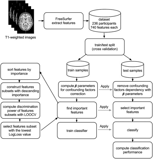
Schematic flowchart of the classification scheme.

Confounding Factor Corrections

Features used in classification depended not only on group status (dyslexic vs. control participants) but also on other group‐unrelated factors such as country, field strength (1.5 vs. 3T scanner), coil (32 channel vs. 12 channel vs. birdcage), sex, age and total intracranial volume (TIV). There was no data dependency on participant's age, while other confounding factors were regressed from the data using a general linear model (GLM) as described previously [Dukart et al., 2011; Płoński et al., 2014]. Feature selection and classifier training were performed on corrected data.

Feature Selection Procedure

Since a universally optimal feature selection method is lacking, the following feature selection algorithms were compared: t‐test [Haury et al., 2011], Information Gain (IG) [Duch et al., 2003], Random Forest Variable Importance (RF var. imp.) [Breiman, 2001]. The selection algorithms provided information about feature importance, however information about the optimal number of features was not available with such a simple procedure. Therefore, subsets with increasing numbers of selected features were created, starting with the most significant and adding others sequentially by descending significance order. The optimal number of features was chosen as the subset with the lowest LogLoss discrimination power metric evaluated using classifier and internal LOOCV on training samples, in a manner similar to that of Eskildsen et al. [2015]. The feature selection procedure was repeated on each CV iteration. Feature selection using inner LOOCVs avoids overfitting for the final classifier training [Cui et al., 2016].

Our dataset has a smaller number of samples (i.e., participants) than features, hence a stability problem arises—in each CV iteration different features might be selected as the most significant [Kalousis et al., 2007]. Thus, we monitored the stability of selection algorithm with the Jaccard index; additionally we computed the feature selection frequency across all CV iterations [Eskildsen et al., 2015]. The Jaccard stability index can be used to select an optimal classification method from among several cases of similar discrimination power [Kalousis et al., 2007].

Classifiers

The classification algorithm was trained using the features selected as described above. A universal optimal classification algorithm that outperforms other algorithms on all datasets does not exist. Therefore, several algorithms were reviewed: Logistic Regression (LR), Support Vector Machine (SVM) with linear kernel [Hastie et al., 2009] and Random Forest (RF) [Breiman, 2001]. Both, SVM and LR were used with default parameters values, whereas 100 trees were used in RF algorithm. We measured classification performance with receiver operating characteristic (ROC) curves, areas under the ROC curves (AUC) and their accuracy (ACC). Additionally, we used a permutation significance test to check that the classifier outperformed random guessing to determine whether the accuracy and AUC obtained above were significantly higher than values expected by chance [Ojala and Garriga, 2010].

The classification framework scheme is presented in Figure 1. Importantly, in every step of classification framework the training and test sets were kept distinct. All computations from classification framework were performed in R environment [R Core Team, 2012].

RESULTS

The performance of each combination of feature selection and classification algorithms for the total sample is presented in Table 1. Almost all combinations give significantly better than chance performance with AUC and ACC around 65%. However, the most stable feature selection in all CV iterations between control and dyslexia classifiers was seen for the t‐test and for Logistic Regression (LR). Table 1 presents P‐values for AUC and ACC based on permutation testing with 100 repetitions.

Table 1.

Classification performance computed on LOOCV and 10‐fold CV repeated 100 times (mean and 95% confidence bounds) for different combinations of selection and classification algorithms together with permutation‐based P‐values

Method	AUC [conf. interv]	P‐value (AUC)	ACC [conf. interv]	P‐value (ACC)	Stability (Jaccard index)
LOOCV
t‐test, LR	0.65	0.01	0.64	0.01	0.93
t‐test, SVM	0.6	0.02	0.62	0.01	0.95
t‐test, RF	0.62	0.01	0.62	0.01	0.91
IG, LR	0.39	ns	0.52	ns	0.78
IG, SVM	0.6	0.01	0.61	0.01	0.88
IG, RF	0.68	0.01	0.65	0.01	0.86
RF var. imp., LR	0.53	ns	0.57	0.04	0.25
RF var. imp., SVM	0.63	0.01	0.65	0.01	0.48
RF var. imp., RF	0.67	0.01	0.67	0.01	0.43
10‐fold CV
t‐test, LR	0.66 [0.63–0.69]	0.01	0.65 [0.61–0.67]	0.01	0.71
t‐test, SVM	0.61 [0.57–0.66]	0.02	0.62 [0.58–0.65]	ns	0.7
t‐test, RF	0.61 [0.56–0.66]	<0.01	0.61 [0.58–0.64]	0.01	0.68
IG, LR	0.56 [0.50–0.62]	0.05	0.58 [0.56–0.63]	ns	0.25
IG, SVM	0.63 [0.58–0.68]	0.02	0.62 [0.58–0.67]	0.02	0.46
IG, RF	0.66 [0.61–0.70]	0.01	0.65 [0.60–0.69]	0.01	0.43
RF var. imp., LR	0.57 [0.51–0.63]	0.03	0.59 [0.56–0.62]	ns	0.18
RF var. imp., SVM	0.61 [0.54–0.67]	ns	0.61 [0.58–0.65]	0.04	0.34
RF var. imp., RF	0.65 [0.60–0.69]	0.01	0.64 [0.61–0.68]	0.01	0.34

ns ‐ not significant (P > 0.05), LR – Logistic Regression, SVM – Support Vector Machine, RF – Random Forest, IG – Information Gain, RF var. imp. – Random Forest Variable Importance.

Table 2.

Features selected by t‐test combined with LR with percentage occurrence in CV iterations for features selected at least in half of the 10‐fold CV iterations and in LOOCV

Region	Hemi	Measure	Selection frequency for LOOCV
			(10‐fold CV)	Discrimination weights
The same in LOOCV and 10‐fold CV
Middle temporal gyrus	L	Folding index	100 (98.1)%	1.201
Planum polare of the superior temporal gyrus	L	Mean curvature	100 (99.9)%	0.327
Transverse frontopolar gyri and sulci	L	Mean curvature	100 (100)%	0.399
Fronto‐marginal gyrus (of Wernicke) and sulcus	L	Area	100 (100)%	−0.368
Lateral aspect of the superior temporal gyrus	L	Mean curvature	100 (100)%	0.238
Subparietal sulcus	L	Mean curvature	44.1 (98.3)%	0.193
Selected only in 10‐fold CV
Fronto‐marginal gyrus (of Wernicke) and sulcus	R	Volume	94.80%
Orbital gyrus	L	Thickness	95.70%
Orbital gyrus	L	Mean curvature	86.50%
Planum polare of the superior temporal gyrus	R	Mean curvature	75.40%
Subparietal sulcus	L	Folding index	71.60%
Orbital gyrus	R	Mean curvature	61.20%

On the basis of these results, we took the t‐test combined with LR to be superior to other algorithms for analysis of our dataset. All classification analyses are therefore based on these two statistical criteria. The features selected with t‐test combined with LR for LOOCV and 10‐fold CV are presented in Table 2. Figure 2A depicts common features, selected by both LOOCV and 10‐fold CV. All were located in the left hemisphere and most were related to geometric characteristics of the cortex, that is, its folding and curvature. Due to the multivariate character of the analysis, which also considers interregional correlations, each selected feature should be interpreted in the context of the entire discriminating pattern and not in isolation. Nevertheless, for a more precise characterization of the results obtained, boxplots of six common features, adjusted for confounding factors, are presented for control and dyslexic subjects (Fig. 2B). Dyslexic children had higher mean curvature in the left superior temporal gyrus and planum polare, left subparietal sulcus and left transverse frontopolar gyrus and sulcus than the control group. With respect to the folding index, higher values in dyslexic children than the control group were observed in the left middle temporal gyrus. Additionally in the left frontal lobe, the surface area of the fronto‐marginal gyrus and sulcus was lesser in the dyslexic group.

Figure 2.

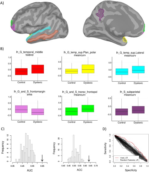
A. Selected features common for 10‐fold CV and LOOCV displayed on an inflated left hemisphere cortex_330117V template from Brainstorm (B) and their boxplots. C. Label permutation test of the t‐test, LR classifier (the performance of a classifier without permuted labels is marked with an arrow) D. comparison of ROC curves of classifier trained with selected features vs. trained with random features, all permutation tests were repeated 100 times. [Color figure can be viewed at http://wileyonlinelibrary.com]

To assess significance of classification system we used label and feature permutation tests. The performance comparison of classification system (t‐test, LR) with classification system learned with random labels is presented in Figure 2C. The proposed method is significantly better than random classifier on both metrics with P‐value < 0.01. The comparison of classifier trained using selected features versus trained with random features is presented in Figure 2D. The ROC curves obtained for the classifier trained with selected features are far more significant than those obtained with classifiers trained on randomly chosen features.

DISCUSSION

The goal of this study was to gain insights into grey matter differences between typical and reading impaired children. A multivariate approach was used for the first time on T1‐weighted images in a large multisite sample of children [Jednoróg et al., 2015] that took into account a variety of cortical morphological measures, including volumetric (i.e., volume, thickness and area) and geometric (i.e., folding index and mean curvature) measures.

Classification into control vs. dyslexic subjects achieved above chance accuracy after principled feature selection and assessment of classification algorithm accuracy. The best performance and greatest stability was found for the t‐test and Logistic Regression classifier where AUC = 0.66 and ACC = 0.65 in the case of 10‐fold CV, and AUC = 0.65 and ACC = 0.64 using LOOCV. Classification performance is less than that obtained using similar multivariate analyses in major neurological disorders such as Alzheimer's disease, where AUC is often above 90% [for e.g., Liu et al., 2012]. However, dyslexia is a more heterogeneous syndrome [Jednoróg et al., 2014; Talcott et al., 2013] and there is little consistency in the results of previous univariate grey matter studies. Our results therefore are the first to convincingly demonstrate a distinct grey matter pattern of abnormality for this developmental disorder. In a similarly heterogeneous syndrome—autism spectrum disorder—multivariate classification analyses have failed to find even this degree of classification accuracy between those with and without the disorder [Haar et al., 2016]. Conversely, in a recent study [Cui et al., 2016] a classifier based on white matter measures achieved much better accuracy (83.6%) distinguishing between dyslexic and control children, which might imply that these tissue properties are better biomarkers of dyslexia. However, the classifier was based on a small cohort (28 dyslexic and 33 controls) of children, which could have inflated decoding accuracies because of wider decoding accuracy distribution characteristic for small samples [Haar et al., 2016]. Further, the generalization of the results was tested only with LOOCV, which might give estimates of prediction error that are more variable than other forms of crossvalidation including 10‐fold CV [Hastie et al., 2009]. Similarly high accuracy (80%) was found by Tamboer et al. [2016], who used linear SVM and LOOCV on grey matter volume derived from structural images of 22 control and 27 dyslexic students, mostly women. However, when the classifier was tested on an independent large sample of young adults, the classification performance dropped to 59%, since large percentage of false alarms was found.

In our study, most of the features that discriminate between dyslexic and control children are related to geometric properties of the cortex, with generally higher mean curvature and a greater folding index characterizing the dyslexic group. The brain areas with such characteristics are exclusively situated in the left hemisphere, including areas previously implicated in dyslexia such as certain classical language areas (i.e., the superior temporal and middle temporal gyri) as well as prefrontal and parietal regions. Higher mean curvature and greater folding index both indicate more complex folded cortex than usual. Our results can therefore be considered as an in vivo replication of Galaburda and Kemper, 1979; Galaburda et al., 1985 findings of cortical microgyrias situated near the Sylvian fissure of the left hemisphere in dyslexic brains. All features included in our classification are corrected for confounding factors, including total intracranial volume, thus the increased folding and mean curvature in dyslexic is not simply a consequence of larger brain size. Our findings are consistent with a recent report of atypical sulcal patterns in left parieto‐temporal and occipitotemporal regions in children with a clinical diagnosis of dyslexia [Im et al., 2016]. In these regions dyslexic children had more sulcal basins of smaller size than the control group. Neither Im et al., nor we find dyslexia vs. non‐dyslexia group differences in the right hemisphere. Im et al. argued that in contrast to morphometric measures, sulcal pattern measurements may better reflect genetic influences on cortical development (i.e., neuronal migration) since the global pattern of primary gyri and sulci is determined prenatally and shows relatively little change during postnatal development [Meng et al., 2014]. Thus, our results support the hypothesis that an atypical sulcal pattern with extra folds in left hemispheric perisylvian regions constitute a biomarker of dyslexia.

Lastly, this study being a multisite study, it suffers from a number of limitations. The data was merged from five different studies carried out on four scanners with different scanning parameters in three countries, which might have introduced error variance to the results. To reduce multisite bias, we included covariates in the GLM model to improve data integrity [Chen et al., 2014], however one cannot exclude the possibility that a less heterogeneous dataset might result in better classification accuracies. Additionally, children came from different social backgrounds, yet this variable could not be properly controlled for, as the information about parental education and profession was not available for the entire sample.

Together with other nuisance variables, sex was regressed from the data because splitting the group by sex decreased the reliability of the analyses. Future studies with larger sample sizes would benefit from treating it as a variable of interest, since there is now some evidence suggesting that the neural basis of developmental dyslexia may to some extent differ between males and females [Altarelli et al., 2013, 2014; Clark et al., 2014; Evans et al., 2014].

To conclude, our study shows that developmental dyslexia is characterized of distinct pattern of grey matter abnormality, which allows for moderate classification accuracy into dyslexic and non‐dyslexic individuals. Dyslexic children had generally higher mean curvature and a greater folding index of left hemispheric brain regions previously linked with language processing.

REFERENCES

- Altarelli I, Monzalvo K, Iannuzzi S, Fluss J, Billard C, Ramus F, Dehaene‐Lambertz G (2013): A functionally guided approach to the morphometry of occipitotemporal regions in developmental dyslexia: Evidence for differential effects in boys and girls. J Neurosci 33:11296–11301. [DOI] [PMC free article] [PubMed] [Google Scholar]
- Altarelli I, Leroy F, Monzalvo K, Fluss J, Billard C, Dehaene‐Lambertz G, et al. (2014): Planum temporale asymmetry in developmental dyslexia: Revisiting an old question. Hum Brain Mapp 35:5717–5735. [DOI] [PMC free article] [PubMed] [Google Scholar]
- Bogdanowicz M, Jaworowska A, Krasowicz‐Kupis G, Matczak A, Pelc‐Pękala O, Pietras I, Stańczak J, Szczerbiński M (2008) Diagnoza dysleksji u uczniów klasy III szkoły podstawowej. Warszawa: Pracownia Testów Psychologicznych. [Google Scholar]
- Breiman L (2001): Random forests. Mach Learn 45:5–32. [Google Scholar]
- Casanova MF, Araque J, Giedd J, Rumsey JM (2004): Reduced brain size and gyrification in the brains of dyslexic patients. J Child Neurol 19:275–281. [DOI] [PubMed] [Google Scholar]
- Chang BS, Ly J, Appignani B, Bodell A, Apse KA, Ravenscroft RS, Sheen VL, Doherty MJ, Hackney DB, O'Connor M, Galaburda AM, Walsh CA (2005): Reading impairment in the neuronal migration disorder of periventricular nodular heterotopia. Neurology 64:799–803. [DOI] [PubMed] [Google Scholar]
- Chen J, Liu J, Calhoun VD, Arias‐Vasquez A, Zwiers MP, Gupta CN, Franke B, Turner JA (2014): Exploration of scanning effects in multi‐site structural MRI studies. J Neurosci Methods 230:37–50. [DOI] [PMC free article] [PubMed] [Google Scholar]
- Clark KA, Helland T, Specht K, Narr KL, Manis FR, Toga AW, Hugdahl K (2014): Neuroanatomical precursors of dyslexia identified from pre‐reading through to age 11. Brain 137:3136–3141. [DOI] [PMC free article] [PubMed] [Google Scholar]
- Cui Z, Xia Z, Su M, Shu H, Gong G (2016): Disrupted white matter connectivity underlying developmental dyslexia: A machine learning approach. Hum Brain Mapp 37:1443–1458. [DOI] [PMC free article] [PubMed] [Google Scholar]
- Dale AM, Fischl B, Sereno MI (1999): Cortical surface‐based analysis. I. Segmentation and surface reconstruction. Neuroimage 9:179–194. [DOI] [PubMed] [Google Scholar]
- Destrieux C, Fischl B, Dale A, Halgren E (2010): Automatic parcellation of human cortical gyri and sulci using standard anatomical nomenclature. Neuroimage 53:1–15. [DOI] [PMC free article] [PubMed] [Google Scholar]
- Duch W, Biesiada J, Winiarski T, Grudziński K, Grąbczewski K (2003): Feature selection based on information theory filters. Adv Soft Comput 19:173–178. [Google Scholar]
- Dukart J, Schroeter ML, Mueller K, Alzheimer's Disease Neuroimaging Initiative (2011): Age correction in dementia–matching to a healthy brain. PLoS One 6:e22193. [DOI] [PMC free article] [PubMed] [Google Scholar]
- Eskildsen SF, Coupé P, Fonov V, Pruessner JC, Collins DL (2015): Structural imaging biomarkers of Alzheimer's disease: Predicting disease progression. Neurobiol Aging 36 Suppl 1:S23–S31. [DOI] [PubMed] [Google Scholar]
- Evans TM, Flowers DL, Napoliello EM, Eden GF (2014): Sex‐specific gray matter volume differences in females with developmental dyslexia. Brain Struct Funct 219:1041–1054. [DOI] [PMC free article] [PubMed] [Google Scholar]
- Finch AJ, Nicolson RI, Fawcett AJ (2002): Evidence for a neuroanatomical difference within the olivo‐cerebellar pathway of adults with dyslexia. Cortex 38:529–539. [DOI] [PubMed] [Google Scholar]
- Fischl B, Sereno MI, Dale AM (1999): Cortical surface‐based analysis. II: Inflation, flattening, and a surface‐based coordinate system. Neuroimage 9:195–207. [DOI] [PubMed] [Google Scholar]
- Frye RE, Liederman J, Malmberg B, McLean J, Strickland D, Beauchamp MS (2010): Surface area accounts for the relation of gray matter volume to reading‐related skills and history of dyslexia. Cereb Cortex 20:2625–2635. [DOI] [PMC free article] [PubMed] [Google Scholar]
- Galaburda AM, Kemper TL (1979): Cytoarchitectonic abnormalities in developmental dyslexia: A case study. Ann Neurol 6:94–100. [DOI] [PubMed] [Google Scholar]
- Galaburda AM, Sherman GF, Rosen GD, Aboitiz F, Geschwind N (1985): Developmental dyslexia: Four consecutive patients with cortical anomalies. Ann Neurol 18:222–233. [DOI] [PubMed] [Google Scholar]
- Galaburda AM, Menard MT, Rosen GD (1994): Evidence for aberrant auditory anatomy in developmental dyslexia. Proc Natl Acad Sci USA 91:8010–8013. [DOI] [PMC free article] [PubMed] [Google Scholar]
- Haar S, Berman S, Behrmann M, Dinstein I (2016): Anatomical Abnormalities in Autism? Cereb Cortex 26:1440–1452. [DOI] [PubMed] [Google Scholar]
- Hastie T, Friedman J, Tibshirani R (2009): The elements of statistical learning. New York: Springer Verlag. [Google Scholar]
- Haury AC, Gestraud P, Vert JP (2011): The influence of feature selection methods on accuracy, stability and interpretability of molecular signatures. PLOS One 6:e28210. [DOI] [PMC free article] [PubMed] [Google Scholar]
- Humphreys P, Kaufmann WE, Galaburda AM (1990): Developmental dyslexia in women: Neuropathological findings in three patients. Ann Neurol 28:727–738. [DOI] [PubMed] [Google Scholar]
- Im K, Raschle NM, Smith SA, Ellen Grant P, Gaab N (2016): Atypical Sulcal Pattern in Children with Developmental Dyslexia and At‐Risk Kindergarteners. Cereb Cortex 26:1138–1148. [DOI] [PMC free article] [PubMed] [Google Scholar]
- Jednoróg K, Gawron N, Marchewka A, Heim S, Grabowska A (2014): Cognitive subtypes of dyslexia are characterized by distinct patterns of grey matter volume. Brain Struct Funct 219:1697–1707. [DOI] [PMC free article] [PubMed] [Google Scholar]
- Jednoróg K, Marchewka A, Altarelli I, Monzalvo Lopez AK, van Ermingen‐Marbach M, Grande M, Grabowska A, Heim S, Ramus F (2015): How reliable are gray matter disruptions in specific reading disability across multiple countries and languages? Insights from a large‐scale voxel‐based morphometry study. Hum Brain Mapp 36:1741–1754. [DOI] [PMC free article] [PubMed] [Google Scholar]
- Jenner A, Rosen GD, Galaburda AM (1999): Neuronal asymmetries in the primary visual cortex of dyslexic and non‐dyslexic brains. Ann Neurol 46:189–196. [DOI] [PubMed] [Google Scholar]
- Kalousis A, Prados J, Hilario M (2007): Stability of feature selection algorithms: A study on high‐dimensional spaces. Knowl Inf Syst 12:95–116. [Google Scholar]
- Küspert P, Schneider W (1998) Würzburger Leise Leseprobe (WLLP). Göttingen: Hogrefe. [Google Scholar]
- Lefavrais P (1967) Test de l'alouette: Manuel. Paris: Les éditions du centre de psychologie appliquée. [Google Scholar]
- Linkersdörfer J, Lonnemann J, Lindberg S, Hasselhorn M, Fiebach CJ (2012): Grey matter alterations co‐localize with functional abnormalities in developmental dyslexia: An ALE meta‐analysis. PLoS One 7:e43122. [DOI] [PMC free article] [PubMed] [Google Scholar]
- Liu M, Zhang D, Shen D, Alzheimer's Disease Neuroimaging Initiative (2012): Ensemble sparse classification of Alzheimer's disease. Neuroimage 60:1106–1116. [DOI] [PMC free article] [PubMed] [Google Scholar]
- Lyon GR, Shaywitz SE, Shaywtiz BA (2003): A definition of dyslexia. Ann Dyslexia 53:1–14. [Google Scholar]
- Ma Y, Koyama MS, Milham MP, Castellanos FX, Quinn BT, Pardoe H, Wang X, Kuzniecky R, Devinsky O, Thesen T, Blackmon K (2014): Cortical thickness abnormalities associated with dyslexia, independent of remediation status. Neuroimage Clin 7:177–186. [DOI] [PMC free article] [PubMed] [Google Scholar]
- Meng Y, Li G, Lin W, Gilmore JH, Shen D (2014): Spatial distribution and longitudinal development of deep cortical sulcal landmarks in infants. Neuroimage 100:206–218. [DOI] [PMC free article] [PubMed] [Google Scholar]
- Ojala M, Garriga GC (2010): Permutation tests for studying classifier performance. J Mach Learn Res 11:1833–1863. [Google Scholar]
- Płoński P, Gradkowski W, Marchewka A, Jednoróg K, Bogorodzki P (2014): Dealing with the heterogeneous multi‐site neuroimaging data sets: A discrimination study of children dyslexia. Brain Inf Health 471–480. [Google Scholar]
- R Core Team (2012). R: A language and environment for statistical computing. Vienna, Austria: R Foundation for Statistical Computing; ISBN 3‐900051‐07‐0, URL http://www.R-project.org/ [Google Scholar]
- Repscher S, Grande M, Heim S, van Ermingen M, Pape‐Neumann J (2012): Entwicklung parallelisierter Wortlisten zur Verlaufsdiagnostik bei dyslektischen Kindern. Sprache Stimme Gehör 36:33–39. [Google Scholar]
- Richlan F, Kronbichler M, Wimmer H (2013): Structural abnormalities in the dyslexic brain: A meta‐analysis of voxel‐based morphometry studies. Hum Brain Mapp 34:3055–3065. [DOI] [PMC free article] [PubMed] [Google Scholar]
- Tamboer P, Vorst HC, Ghebreab S, Scholte HS (2016): Machine learning and dyslexia: Classification of individual structural neuro‐imaging scans of students with and without dyslexia. Neuroimage Clin 11:508–514. [DOI] [PMC free article] [PubMed] [Google Scholar]
- de Vasconcelos Hage SR, Cendes F, Montenegro MA, Abramides DV, Guimarães CA, Guerreiro MM (2006): Specific language impairment: Linguistic and neurobiological aspects. Arq Neuropsiquiatr 64:173–180. [DOI] [PubMed] [Google Scholar]