

Abstract
In anticipation of the expanding appreciation for air quality models in health outcomes studies, we develop and evaluate a reduced-complexity model for pollution transport that intentionally sacrifices some of the sophistication of full-scale chemical transport models in order to support applicability to a wider range of health studies. Specifically, we introduce the HYSPLIT average dispersion model, HyADS, which combines the HYSPLIT trajectory dispersion model with modern advances in parallel computing to estimate ZIP code level exposure to emissions from individual coal-powered electricity generating units in the United States. Importantly, the method is not designed to reproduce ambient concentrations of any particular air pollutant; rather, the primary goal is to characterize each ZIP code’s exposure to these coal power plants specifically. We show adequate performance towards this goal against observed annual average air pollutant concentrations (nationwide Pearson correlations of 0.88 and 0.73 with and PM2.5, respectively) and coal-combustion impacts simulated with a full-scale chemical transport model and adjusted to observations using a hybrid direct sensitivities approach (correlation of 0.90). We proceed to provide multiple examples of HyADS’s single-source applicability, including to show that 22% of the population-weighted coal exposure comes from 30 coal-powered electricity generating units.
Keywords: Reduced complexity model, source impacts, HYSPLIT, air pollution exposure, PM2.5
1. Introduction
Millions of people worldwide die prematurely and/or suffer from diseases associated with exposure to polluted air. Besides being tragic in their own right, deaths and diseases impart vast costs on the world and United States economies [1, 2].
Developed and developing nations alike have reacted over recent decades by instituting policies intended to curb their citizens’ exposure to air pollution; recent policies target particulate matter with aerodynamic diameter less than 2.5 μm (PM2.5). Many of these policies regulate point air pollution sources, which comply with regulations through discrete actions such as switching fuels, installing emissions controls, and/or changing their usage patterns [3, 4]. Recent evaluations have shown that these approaches have been beneficial to both air quality and health [5, 6, 7]; however, future policies will rely on finer margins for improving air quality in developed countries, and cost-effective policies will require targeted emissions reductions at sources that have the highest potential to impact human health. Similarly, air quality management in developing countries would benefit from identifying sources that contribute disproportionately to adverse impacts to human health.
Recent studies have quantified source-specific impacts on air quality and health [8, 9, 10, 11, 12]. One approach used by these studies, observation-based source apportionment methods, offers the benefits of using measured air quality concentrations and allowing of formal statistical uncertainty quantification in the estimates. Recent developments in multivariate receptor modeling approaches offer the added ability to estimate source contributions at locations that do not have monitors [13, 14]. Observation-based approaches, however, are limited in their ability to reflect spatial variability in sources [15, 16] and rely on source profiles that are variable between locations [17] or require researcher judgment linking principal-component-type rotated variables with known source profiles in factor analytical methods [18, 19, 20]. Further, the methods have difficulty parsing impacts on secondary pollutant species such as sulfate () and nitrate () and do not distinguish individual sources within source categories, which limits the methods’ applicability to comparisons of interventions implemented on individual sources.
Chemical transport models (CTMs), which simulate atmospheric constituent transport, diffusion, deposition, and reactions across a 3-D grid and over time, have been adapted to estimate impacts from source-specific emissions on air quality [21]. Researchers have applied brute force calculations of source impacts [22], direct calculation of sensitivities [12] and adjoint [23, 24] approaches to quantify air quality and health impacts of emission sources. These methods benefit from detailed chemistry and physics parameterizations that allow for the apportionment of secondary species and fine resolution (typically on the order of 4-36 km); however, they require extensive computing resources to run, making them impractical for investigating single source-receptor relationships for a large number of sources over multi-year time periods.
Plume dispersion models offer an alternative to observation-based source apportionment methods and CTMs [25, 26]. While more limited in their abilities to fully capture complex atmospheric processes such as chemical transformation and deposition, these models are useful for determining spatial impacts of large numbers of sources because of their reduced computational burden and scalability. Models of this type have been applied to many problems involving the linking of individual sources and receptors, including real-time forecasting of radioactive emissions impacts from Japan’s Fukushima nuclear facility in 2011 [27, 28] and impacts of emissions from the 2010 Eyjafjallajökull volcano eruption in Iceland [29].
Recent development in so-called “reduced-form” or “reduced-complexity” models offers expanded practicality of source-specific studies by intentionally simplifying some of the complexity of full-scale CTMs in exchange for a computational scalability that supports estimation of fine-scale (e.g., ZIP code-level) impacts from a large number of individual sources over long periods [30, 31, 32, 33]. These models typically rely on plume dispersion models and/or CTM outputs to approximate pollution transport and chemistry. The ability to model individual source impacts using atmospheric chemistry tools has the potential to improve on approaches taken in recent health and population studies that have employed much simpler approaches to estimating population exposure, such as power plant proximity [34, 35].
We present and evaluate a method for quantifying individual source impacts on populations with the ultimate goal of informing future intervention and health analyses with ZIP code level estimates of exposure to coal power plant emissions in the United States. The development follows a spirit similar to that of reduced-complexity CTMs, wherein we combine an intentionally simplified characterization of pollution transport via the HYSPLIT trajectory model with recent advancements in parallel computing to model ZIP code-level impacts from individual power plants in the U.S. The method was developed to have 1) broad spatial coverage at fine spatial resolution, 2) the ability to estimate contributions of hundreds of individual point sources to exposure, and 3) the ability to simulate changing exposure over time with changing emissions and meteorology. These goals are motivated by the desire to advance downstream health-impact evaluations of pollution intervention studies that require links between point sources and affected populations. We evaluate the model’s ability to capture spatial and temporal variability in exposure attributable to emissions from individual coal-fueled electricity generating units operating in the United States in 2005 and 2012, and we provide example applications to identify sources that impart the largest impacts on populations.
2. Methods
We define coal exposure as the influence of emissions from coal electricity generating units (EGUs) on ZIP codes, and distinguish it from total exposure, which refers to pollutants from all sources. The definition is sufficiently broad so as to avoid referring to specific pollutant species (e.g., SO2, PM2.5, etc.) in anticipation of informing health studies that seek to establish links between adverse health outcomes and air pollution sources. ZIP code level estimates are the target of this analysis because databases used in air pollution epidemiology studies are often structured on ZIP codes or larger administrative units (e.g., county, state, or province).
2.1. HYSPLIT average dispersion
We simulate exposure to coal power plants in the continental United States using a method called the HYSPLIT average dispersion (HyADS) approach. HYSPLIT is an air parcel trajectory and dispersion model maintained by the National Oceanic and Atmospheric Administration (NOAA) Air Resources Laboratory [25, 26]. HYSPLIT uses wind fields to trace air parcel transport through the atmosphere [25, 26]. In its forward mode, HYSPLIT estimates air parcel trajectories emanating from single point sources defined by horizontal and vertical coordinates.
For years 2005 and 2012, we used the SplitR [36] package in R to simulate the dispersion of 100 parcels emitted every six hours (12:00 a.m., 6:00 a.m., 12:00 p.m., and 6:00 p.m.—each release constitutes an “emissions event”) from each coal electricity generating unit using HYSPLIT—100 was chosen to balance computational efficiency and model complexity. Starting positions for each emissions event were based on each source’s stack location and height. Parcel locations were calculated for 10 days after each emissions event based on NCEP reanalysis wind speeds and directions [37]. Hourly parcel locations were discarded in three instances: 1) in hours 0 and 1 to limit unrealistic near-source ground-level impacts, 2) after they reached a height of zero (no resuspension), and 3) at altitudes above the planetary boundary layer. Monthly gridded boundary layer heights were retrieved from 20th Century Reanalysis data [38].
Retained hourly air parcel locations were summed by month over a fine (0.19°×0.19°; approximately 22 km latitude×16 km longitude in the center of the country) grid. Parcel concentrations were calculated in each grid cell as the number of parcels per volume, where area was assigned the nominal value of one (all grid cells had the same area) and height was the monthly boundary layer height. Gridded concentrations were spatially averaged over ZIP codes using the over command in the sp R package [39].
The resulting unit-less concentration metrics link individual coal units directly with particle concentrations in ZIP codes and form a transfer coefficient matrix (TCM; also called a source-receptor matrix) of the form TCMi,j,t, where (i,j) refer to the receptors and sources in the matrix, and t refers to time at which the matrix was calculated.[27, 30, 40]. Thus, , the transfer coefficient matrix for HyADS, constitutes a numerical representation of pollutant transport from each power plant j to each ZIP code i in each month t. Annual HyADS exposure from each unit is defined as:
| (1) |
Where t represents months and emissionst,j is the monthly SO2 emissions from coal EGU unit j. Total exposure to emissions from all units at each location i is defined as:
| (2) |
Where J is the total number of sources. HyADS calculates exposure as the summed influence of thousands of parcel trajectories to capture the sum of 6-hourly impacts and counter potential biases stemming from uncertainty in individual wind fields and parcel starting points [38]. The model can be run entirely from the R package hyspdisp [41], which contains functions that parallelize functions in SplitR and spatially allocate HyADS exposures to ZIP codes. The approach yields units of emissions-weighted parcel concentrations, and we refer to the outputs and as HyADS relative coal exposure. HyADS exposure fields quantify each area’s exposure to emissions, and do not represent estimates of exposure to any single atmospheric constituent such as PM2.5, , or SO2.
2.1.1. Coal facility emissions
The HYSPLIT-based approach for quantifying coal exposure leverages emissions measured at the source and detailed information about individual source stacks. Daily unit-level SO2 emissions magnitudes were downloaded from US Environmental Protection Agency’s (EPA) Air Markets Program Database (AMPD) and summed to monthly emissions [42]. Stack heights were retrieved from the EPA’s 2005 and 2011 National Emissions Inventories [43] and matched to AMPD units. In 2005 (2012), the matched inventory contained 780 (818) units, leaving 256 (191) unmatched. Unmatched units were assigned the average stack height of the matched units (150 m). The use of average stack height has little impact on the overall spatial distribution of emissions impacts from individual facilities, but has larger impacts on ZIP codes in close proximity to stacks (see SI for further discussion). The 1,036 (1,009) units in operation in 2005 (2012) comprised 505 (478) facilities (Fig. 1)
Figure 1:
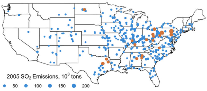
2005 coal electricity generating units sized by SO2 emissions; orange dots denote the 30 units with greatest SO2 emissions in 2005.
2.2. Exposure metric evaluations
HyADS, designed to establish links between sources and receptors, outputs coal exposure in relative concentrations. Relative exposure metrics are useful for certain types of public health studies [44], but may be difficult to interpret in relation to observed ambient measurements. HyADS’s coal impacts spatial distributions can nonetheless be evaluated using observed pollutant concentrations and coal impacts modeled with chemical transport models. Keeping in mind the anticipated use of these exposure fields in health outcomes analyses, we present comparisons of correlations between HyADS and multiple metrics across the entire domain and in specific regions. While this evaluation is limited by the availability of national estimates of spatially refined coal power plant emissions exposure, elevated spatial and temporal correlations between HyADS and the metrics described below provide evidence that the HyADS model captures variability found in these approaches. Relatedly, spatial agreement between changes in these metrics between 2005 and 2012 provides evidence the model captures variability in the change over a period with large emissions change.
2.2.1. CMAQ-DDM Coal Impacts
HyADS’s 2005 exposure field is evaluated against coal emission exposure derived from the Community Multiscale Air Quality model equipped with the direct decoupled method (CMAQ-DDM), which simulates first-order model sensitivities to emissions. In this case, CMAQ-DDM (v5.0.2) was used to estimate model sensitivities of total PM2.5 to coal burning emissions. Coal sources were identified in the National Emissions Inventory (NEI) by the first six digits of the assigned eight- or ten-digit EPA source classification code (SCC). SCCs designate equipment, fuel, facility type, and process. While coal burning sources were not limited in this case to power plants in the CMAQ-DDM application, electricity generation accounted for the overwhelming majority (89%) of coal SO2 emissions in 2005. The results presented here were corrected for bias using both a hybrid optimization approach for improving trace metals concentrations [11] and a correction for improving secondary PM2.5 estimates (, , , and secondary organic carbon)[45]. The results of this observation-adjusted metric for coal exposure were originally presented by Ivey et al., 2015, and we refer to them here as HYBRID-DDM.
The two adjustment methods are briefly described here. First, the hybrid optimization makes use of sequential quadratic programming to minimize the squared error (X2) of the objective function (Eq. 3) while optimizing the source impact adjustment factors Rj:
| (3) |
where are observed concentrations of speciated PM2.5 (i species), are CMAQ modeled concentrations, SAij are CMAQ-DDM estimates of the impact of source j on species i, σ are uncertainties, and Γ is a weighting constant. In Ivey et al. 2015, this function was applied at every monitor in the U.S. with valid PM2.5 speciation data[45]. The optimized Rj at each monitoring site were spatially interpolated using kriging, which provided entire spatial fields of source impact adjustments. The spatial hybrid application was evaluated using 10-fold cross-validation for the kriging step. The accuracy of hybrid-adjusted concentrations for PM2.5, when compared with observations, was improved by approximately 20% across all monitors. High bias in metals concentrations estimates were greatly reduced after hybrid adjustment.
Secondly, while the hybrid adjustment is targeted towards PM2.5 species concentrations that are vulnerable to emissions biases (e.g., primary constituents), the correction for secondary PM2.5 components addresses model uncertainties in gas-particle partitioning and oxidation processes. The chemical species most affected by these modeled processes include , , , and secondary organic carbon. The secondary species adjustment distributes the impact-weighted bias (Di, Eq. 4) in total modeled concentrations of the components across the source impacts [45].
| (4) |
The adjustments (SCij, Eq. 5) are calculated at each monitoring location with available speciated data, then kriged to create spatial fields of adjustment over the entire CMAQ domain.
| (5) |
Since source impacts on secondary species can be negative due to the non-linearities in the sensitivity calculation, negative source impacts do not receive the adjustment. Note that negative source impacts do not indicate negative total concentration. The prediction performance of the corrected concentrations improves significantly, and new biases are near-zero. Readers are referred to the referenced manuscripts for the supplementary equations.
Directly calculated sensitivities, such as those on which HYBRID-DDM are based, are calculated alongside pollution concentrations in chemical transport models. Unlike HyADS and other reduced-complexity approaches, these models include detailed parameterizations for advective and diffusive transport, reactions, and deposition. Therefore, we utilize coal impacts fields from HYBRID-DDM (unit: μg m−3) as a qualified ground truth for the HyADS metric, treated as such because it is an estimate of coal emissions exposure. The comparison, however, is limited because it 1) measures PM2.5 coal exposure (as opposed to total coal exposure simulated by HyADS), and 2) contains a small number of coal emissions sources that are not power plants.
2.2.2. Total exposure—ambient pollution observations
We used annual average PM2.5 and measurements at EPA’s Air Quality System (AQS) sites (AQS parameter codes 88101 and 88403) as observed metrics for total exposure [46]. The two pollutants have been linked historically to negative health outcomes and are the major particulate air pollutants resulting from coal burning emissions in the United States. Ambient concentrations at each monitoring location were assigned to ZIP codes within 10 km, and ZIP code areas that contained multiple monitors were assigned the average of encompassed monitors.
2.2.3. Spatial distribution
We focus on the year 2005 for the base evaluation of HyADS, and subsequently estimate the change in exposure over a period of major nationwide emissions changes between 2005 and 2012. Evaluations are made on the ZIP code level to align with recent health outcomes studies [47, 48]. We use two metrics for correlation: linear (Pearson) and rank-ordered (Spearman), both of which range from −1 to +1. Quantitative comparisons are grouped by regions and restricted to ZIP codes with centroids east of 110° longitude (Fig. SI-1) because of the sparse spatial distribution of coal facilities in the West.
As HyADS offers the ability to estimate coal exposure changes between years, we calculate correlations of the spatial distributions of changing coal exposure and PM2.5 and exposures between 2005 and 2012. We chose these years because the United States saw large emissions decreases from its coal power plants between these years (coal power plant SO2 emissions decreased 64%). HYSPLIT dispersion fields were re-run for each facility using 2012 wind fields. HYBRID-DDM estimated with a consistent approach is not presently available for years after large emissions changes—the latest year available is 2006.
We present multiple examples of HyADS’s ability to identify locations impacted by individual sources. To illustrate how the method might identify impacts of a select number of sources, we computed the HyADS impacts for the 30 units that had the highest SO2 emissions in 2005. Finally, we present of an example approach for rank-ordering individual power plant impacts by estimating each facility’s total population-weighted exposure.
2.2.4. Population-weighted exposure
As a policy-relevant metric of the influence of coal emissions from individual emission sources on populations, we calculate population-weighted exposure (pE) estimates of 2006 population (2005 estimates were not available; 2006 population was used as a proxy for 2005) at each ZIP code (populationi) retrieved from Esri Business Analyst Demographic Data (Esri, Redlands, CA). We calculate each facility’s population-weighted exposure in all ZIP codes (pEi,j), each facility’s total population-weighted exposure (pEj) over all locations I, and total population-weighted exposure from a subset of M facilities (pEM).
| (6) |
| (7) |
| (8) |
While equations for population-weighted metrics traditionally involve normalizing by, for instance, total population, we forgo this step because the units for Ei,j need not be preserved in applications that rely exclusively on spatial variability.
2.2.5. Scaling HyADS to μg m−3
HyADS source-receptor linkages are useful to establish relationships between adverse health outcomes and emissions from individual sources, however, situations may arise for which future researchers prefer impact estimates in physically observable units (example applications and limitations discussed in detail in the Limitations section). In this vein, we present a scaling technique to scale HyADS concentration units to a scale mimicking μg m−3 using region-specific linear relationships with HYBRID-DDM that maintains local variability simulated by HyADS. We apply region-specific conversions of HyADS concentrations to units [μg m−3] using linear relationships with HYBRID-DDM (Fig. 5 and Tab. SI-3):
| (9) |
Where m is the slope, b is the intercept, and ε is the error term. Applying this conversion creates a new metric, HyADSadj, that is calibrated to HYBRID-DDM to have the same units [μg m−3]:
| (10) |
Figure 5:
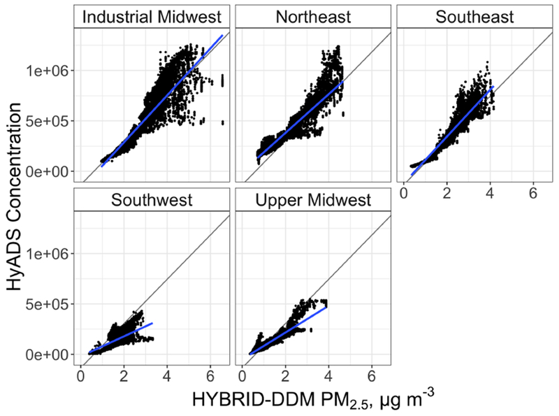
Scatter plots comparing regional HyADS and HYBRID-DDM concentrations and each region’s linear fit. The linear fit for all regions (grey line) provides context for each region’s deviation from the national average. Fit parameters are reported in Tab. SI-3.
Note that while such a rescaling may be advantageous in some situations, it is not strictly required for the HyADS approach to provide useful insights on spatial variability and relative ranking of sources-specific impacts. Furthermore, such rescaling requires either the concurrent availability of a physically-interpretable output (in this case, HYBRID-DDM) to anchor the rescaling or the ability to extrapolate relationships such as those in eq. 9 across other time periods when such physically-interpretable outputs are unavailable. We revisit this point in the discussion on limitations (section 4.1).
2.3. Model availability
All models and data used in this analysis are publicly available for application to sources, locations, and periods outside those investigated here. HyADS runs through an R interface—SplitR—and is parallelized by the hyspdisp R package, which can be used to link dispersion particles to ZIP codes [41, 36]. CMAQ-DDM is available open source through the EPA at https://github.com/USEPA/CMAQ, and scripts for the HYBRID-DDM procedure are available upon request.
3. Results and discussion
3.1. Coal facility emissions
The vast majority of coal facilities in the United States are located in the eastern half of the country, and most eastern states contain several facilities (Fig. 1). The distribution of EGU SO2 emissions by unit is highly right-skewed—of the original 1,036 units, the 30 with the highest emissions in 2005 emitted 21% of the national total. A majority of these largest plants are in the Ohio River Valley; this region contains both the densest group of electricity generating units and most of the largest.
3.2. Spatial exposure distributions
Ambient 2005 concentrations and HyADS and HYBRID-DDM coal exposure metrics are higher in the East and lower in the West; between PM2.5 and spatial distributions (Fig. 2), exhibits a greater disparity between concentrations in the East and West (Fig. 3). HyADS and HYBRID-DDM coal exposure metrics display two distinct bands of elevated influence in the eastern US, both extending to the south and west originating from Pennsylvania. One band travels down the Ohio River Valley, and the other extends through the Southeast into Alabama. The metrics show elevated exposure over eastern Texas. Observed PM2.5 and exhibit elevated concentrations in southern California that are absent in the coal exposure metrics, reflecting established elevated contributions from non-coal sources in the region, such as automobiles, industry, and marine vessels [45, 49]. Similar spatial patterns of air pollution related to coal power plant emissions, particularly the east-west gradient, have been reported in the literature [10, 50, 51, 52, 53].
Figure 2:
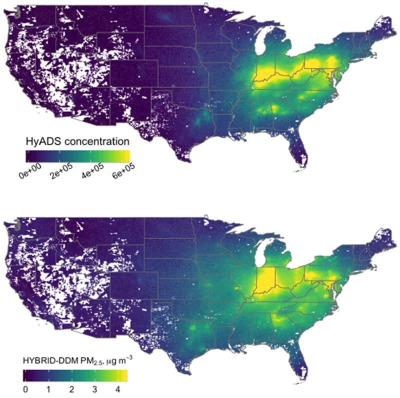
2005 annual average coal exposure metrics with scales set from 0 to the 95th percentile of each metric. HyADS relative concentrations are unitless and correspond to calculated in equation 2.
Figure 3:
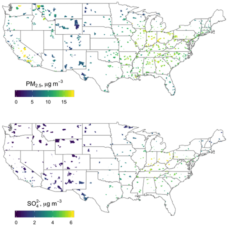
Annual average PM2.5 (left) and (right) observations in 2005 assigned to ZIP codes with centroids within 10 km of each AQS monitor.
3.2.1. Cross-metric evaluations
Correlations between all metrics are generally high (most are greater than 0.70), and most comparisons have similar rank-ordered and linear correlations (Fig. 4, values in Tabs. SI-1 and SI-2). HyADS is highly correlated with HYBRID-DDM—Pearson and Spearman correlations are all equal to or above 0.87 in each of the regions except for the Southwest. The majority of this region is very low exposed with the exception of localized impacts of three large facilities in northeastern Texas. Lower correlations between HyADS and HYBRID-DDM in the Southwest, therefore, are likely more attributable to sparse localized impacts than an inability to capture overall spatial patterns in this region.
Figure 4:
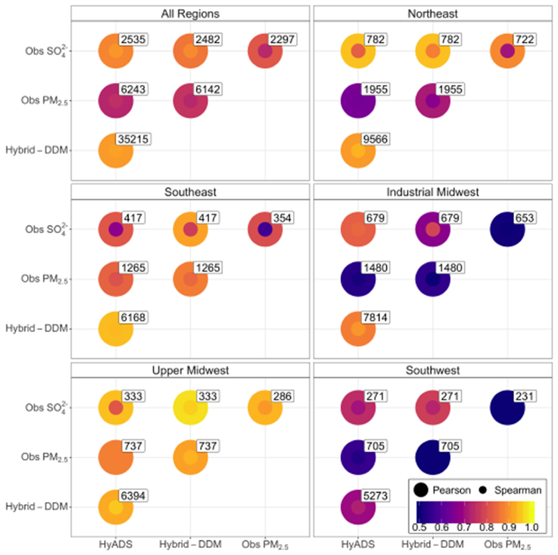
Pearson (linear) and Spearman (rank-ordered) correlations between 2005 annual average coal exposure metrics and monitoring data. Boxed numbers beside each point denote the number of pairs of ZIP codes included in each comparison. Values are reported in Tabs. SI-1 and SI-2.
HyADS (Pearson: 0.88, Spearman: 0.90) and HYBRID-DDM (Pearson: 0.86, Spearman: 0.89) exposures are similarly correlated with observations in the All Regions and most of the individual region comparisons. That HYBRID-DDM tends to be slightly more correlated with observed total exposure metrics—particularly —than HyADS is expected because the method uses these same observations to adjust raw CMAQ-DDM coal emissions sensitivities. Thus, the fact that HyADS exhibits strong correlations with (and HYBRID-DDM) without making explicit use of observations is interpreted as strong evidence that HyADS accurately reflects the spatial distribution of coal exposure.
In All Regions, HyADS is more highly correlated with than PM2.5 (Pearson: 0.73, Spearman: 0.75), a pattern which is repeated in all regions except the Southeast, where HyADS correlations with and PM2.5 are similar. Elevated correlations between all modeled metrics and observed sulfate across All Regions and in most individual regions supports the models’ abilities to capture spatial variability in , an important PM2.5 component formed in the atmosphere from SO2 emissions. In 2005, 72% of nationwide SO2 emissions came from electric utilities [43].
Differences in correlations between observed pollutant species and coal exposure metrics between regions highlight important differences in regional characteristics that impact the abilities of each model to capture spatial variability in coal exposure. For example, correlations between observations and HYBRID-DDM and HyADS coal exposures in the Industrial Midwest and Southwest regions are lower than in other regions. Previous studies have identified contributions of industrial activity and coal mining in the Industrial Midwest as important contributors to ambient pollution and health effects variability [54, 55, 48]. In the Southwest, much of the PM2.5 comes from crustal material and organic matter [56], suggesting that the low correlations are a result of observed spatial variability being driven by sources other than coal-fired power plants. These comparisons underscore the lack of a true gold standard for comparison against the HyADS outputs that model only power plant impacts.
The region-specific scatter-plot in Fig. 5 provides further insight into the relationship between HyADS and HYBRID-DDM. The two models have similar slopes among All Regions, the Northeast, the Industrial Midwest, and the Southeast, with HyADS finding higher concentrations in the Northeast relative to other regions. Slopes are lowest in the Southwest and Upper Midwest, suggesting lower HyADS exposures relative to HYBRID-DDM. An investigation into a set of data points that are causing this lower slope—i.e., the areas in which HYBRID-DDM finds concentrations above 2.8 μg m−3 and HyADS finds impacts greater than 2 × 10⁶ [unitless]—finds that they are primarily concentrated around a few discrete areas (Fig. SI-2). These areas likely highlight sources that are included in the CMAQ emissions inventory for HYBRID-DDM and not for HyADS, potentially including non-utility industry sources. Sources that are included only in the CMAQ emissions inventory are more important in the Upper Midwest and Southwest regions because of the relative scarcity of coal power plants in these regions.
3.2.2. Converting HyADS units to μg m−3 using HYBRID-DDM
The linear relationships observed in Fig. 5 provide an opportunity to transform raw HyADS to the scale of HYBRID-DDM, which may be useful for some applications. As expected when using a model to predict data on which it is trained, normalized mean bias in all regions is less than 3% and error is less than 20% (Tab. SI-3). The 10%, 50%, and 90% quantiles of HyADSadj (0.51, 1.99, and 3.76 μg m−3) and HYBRID-DDM (0.50, 2.08, and 3.78 μg m−3) are similar for locations east of −110° longitude.
Recall that the above conversion relies on contemporaneously-available output with which to rescale the raw HyADS, in this case, HYBRID-DDMin 2005. To evaluate the potential of employing these estimated relationships in 2005 to estimate HyADSadj in years for which HYBRID-DDM is not available, we simulated for an additional year (2006) and calculated for 2006 using Eq. 10. As HYBRID-DDM results are available for this year, we evaluated 2006 against 2006 (evaluation presented in Supplemental Information). In all regions, the evaluation produces a normalized mean bias of 10%, a normalized mean error of 21.5%, and a mean bias of 0.19 μg m−3 (Tab. SI-6). Region-specific normalized mean biases range from −4.1% in the Southwest and 23.7% in the Industrial Midwest.
Application and interpretation of HyADSadj should consider the greater uncertainty in the Upper Midwest and Southwest regions and should interpret results using raw HyADS in addition to HyADSadj. This is suggested because of the previously discussed disparities between the sources included in HYBRID-DDM and HyADS.
3.3. Exposure change over time
HyADS benefits over HYBRID-DDM in that the HYSPLIT dispersion fields can be trivially run at different points in time based on concurrent meteorology—which can be downloaded through the R interface—and emissions from other sources. Characterizing exposure change over multiple years for HYBRID-DDM without fixing other conditions requires additional year-long chemical transport model simulations.
Areas of largest exposure change between 2005 and 2012 (Fig. 6) are located in the eastern United States, similar to areas of greatest coal exposure in 2005 (Fig. 2). HyADS estimates the largest reductions near areas of densest emissions, such as along the Ohio River Valley and Pennsylvania.
Figure 6:
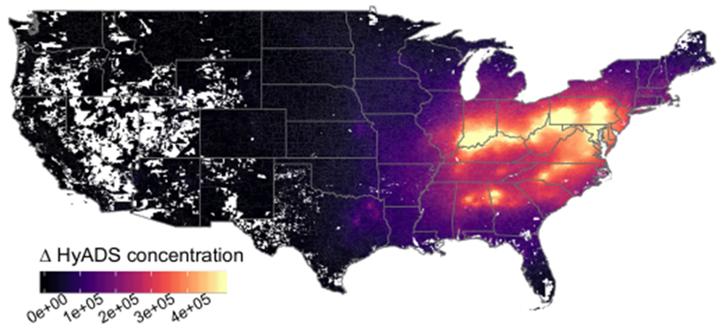
Decreases in HyADS coal exposure between 2005 and 2012. The legend upper limit is set to the 95th percentile of the decrease.
As HYBRID-DDM coal impacts are unavailable after 2006, we evaluate HyADS-simulated exposure changes between 2005 and 2012 using observed concentrations. HyADS changes between 2005 and 2012 are highly correlated with changes over the same period (0.84 (Pearson), 0.87 (Spearman), Fig. SI-3 and Tabs. SI-4 and SI-5). In each individual region, Pearson correlations between HyADS and are all between 0.77 (Industrial Midwest) and 0.97 (Upper Midwest).
Observed concentrations fell by 56%, whereas HyADS exposure declined by 71% across All Regions, which aligns with observed reductions in coal fired power plant emissions of 65%. The larger percentage reduction in coal exposure than observed is consistent with (but not conclusive evidence of) the fact that HyADS only measures exposure attributable to coal power plant SO2 emissions. Further dampening of the response of to SO2 emissions reductions has been reported previously, and has been attributed to the multiple factors that determine concentrations, including SO2 emissions from other sources, emissions of other species, seasonal meteorology, and cloud pH [57, 58].
3.4. Applying HyADS
After running HYSPLIT dispersion fields for each individual source and aggregating their impacts to ZIP codes, HyADS’s transfer coefficient matrix allows for policy-relevant calculations to identify sources that expose populations to their emissions. As in traditional air quality models, two options are available—forward and backward (adjoint) sensitivities. From a forward perspective, facilities can be ranked by their total emissions, and their impacts on populations can be compared spatially. From an adjoint perspective, we start with each facility’s impacts and estimate population-weighted exposure, which can be compared between facilities.
3.4.1. Population-weighted exposure from the top 30 emitting units in 2005
The top 30 emitting units elevate ZIP code exposures throughout the Eastern United States (Fig. 7). HyADS’s 2005 total population-weighted exposure attributable to the top 30 emitting units as a fraction of population-weighted exposure from all units () is 22%, similar to the 21% of total SO2 emissions from these facilities.
Figure 7:
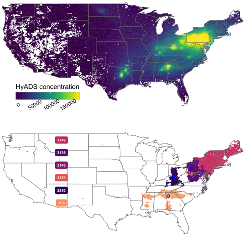
Top: HyADS coal exposure attributable to 30 largest SO2 emitting units in 2005, with the upper legend limit set to the 95th percentile. Bottom: ZIP codes whose maximum population-weighted exposure originates from facilities that have the highest population-weighted exposure. Facility numbers corresponding to FacilityID in the AMPD database are included to aid in the comparison.
3.4.2. Population-weighted exposure by facility
HyADS’s transfer coefficient matrix approach allows for simple estimation of facility-level population-weighted exposure (pEi,j). Each facility’s pEi,j can be compared with other facilities, allowing a ranking of each facility in terms of its impacts on populations. The ZIP codes for which the highest-ranked value of pEi,j was one of these six most influential facilities are depicted in Fig. 7. 7,732 ZIP codes are colored in Fig. 7 representing homes to 78.1 million people, or 26% of the population of the continental United States in 2005. The capability of HyADS to identify the most important point sources for any given area in the modeling domain has direct policy relevance.
4. Implications
The evaluations presented above show consistency between a reduced complexity approach for estimating fine-scale spatial distributions of coal impacts in the United States with observations and chemical-transport modeled coal exposure. The HyADS model has various strengths and weaknesses that should dictate its future applications and evaluations.
4.1. Limitations
An initial limitation is the challenge associated with finding a perfect comparison metric for validating HyADS and HyADSadj. Measurements, receptor modeling, and chemical transport modeling approaches each have uncertainties and are limited in their capacities to identify individual source contributions to exposure. Each, therefore, presents an imperfect point of comparison for the nationwide HyADS approach developed here. The previously published HYBRID-DDM results employ the hybrid adjustment using observations to reduce errors in raw chemistry and transport modeled source impacts, but, while coal impacts adjustment factors were small compared to other sources categories [11], uncertainties remain. The present evaluation of HyADS with HYBRID-DDM is limited by the necessary inclusion of all coal emissions sources in HYBRID-DDM. 89% of emissions from coal sources came from power plants in 2005, and we identified geographic areas where the inclusion of non power-plant sources in comparison metrics was likely to have most impact on the evaluation (Fig. SI-2). Future developments of nationwide coal impacts fields using improved chemical transport and receptor modeling techniques (e.g., multivariate receptor modeling) will enable more complete uncertainty quantification.
A second limitation of HyADS is its unit-less relative concentration outputs. While relative units are useful for identifying exposure distributions and generating contrasts in exposure [44], they are difficult to interpret relative to familiar metrics for ambient concentrations. One possible approach outlined here is to conduct a regression-based calibration between HYBRID-DDM and HyADS to convert the unitless metric into HyADSadj, interpretable in μg m−3. While this rescaling is limited by the availability of modeled quantities to scale against, this conversion can be important for contextualizing model outputs in interpretable units and for comparison of health impact estimates [44]. The converted HyADSadj values simulated here have low bias and error compared to HYBRID-DDM simulated in a separate year, indicating the possibility of using rescaling parameters from one year to provide HyADSadj in years where no CTM output is available. Evaluation of HyADS and HyADSadj changes using alternative exposure metrics across temporal scales is an important ongoing endeavor that will inform future potential applications to health studies.
A third limitation of this implementation of HyADS is that the exposure metric is based only on SO2 emissions. Coal-fueled power plants emit other species (e.g., NOx and mercury) that have been linked to increased air pollution concentrations and adverse health outcomes and have been the focus of regulatory action over recent decades. Future applications and evaluations of HyADS may opt to employ these pollutants as additional exposure metrics.
4.2. Reduced complexity modeling for source-specific exposure studies
HYBRID-DDM and other approaches that employ chemical transport models are powerful tools for simulating air pollution concentrations and source impacts; however, their frameworks are far less flexible for quantifying individual impacts of large numbers of individual sources. HyADS has the ability to quantify impacts from single sources, and the model is relatively fast to set up run using new tools entirely accessible from within R, a widely used computational platform.
The HyADS reduced complexity model is designed in particular for use in health-outcomes studies focusing on specific point sources and on the policies impacting those sources. These studies have the potential to address a different—albeit related—question than the typical epidemiological study that establishes increasing damages with increasing concentrations. The model provides an opportunity for future work that may investigate total exposure to air impacted by emissions from a single source instead of limiting epidemiological evidence to observable pollution species. For example, using HyADS, researchers will be able answer questions such as What impacts do increased exposure to emissions from individual coal power plants have on health? This primary intended use of the method motivated the evaluations focusing on relative ranking of ZIP code exposures, which is distinct from a more traditional evaluation restricted to predictions of ambient concentrations (e.g., of PM2.5), which might be of interest in a different type of study. Early advances in the use of HyADS for this type of investigation appear in Henneman et al., (2018) [44]. While HyADS’s relative units do not allow for a quantification of bias or error relative to ambient concentrations, high spatial correlations (Fig. 4) and visual inspection of the spatial distributions (Fig. 3) along with its reliance on the HYSPLIT model provide strong evidence that HyADS captures transport patterns that align closely with those produced by HYBRID-DDM’s more complex accounting of chemistry and transport.
Various methods have been developed to quantify individual-source impacts on regional and/or national scales, including APEEP[30], InMAP[31], and EASIUR[32]. All three of these models have been shown to reproduce output from chemical transport models at levels similar to accepted performance standards. These models rely on different approximations of chemistry and transport—APEEP employs Gaussian Plume models, InMAP uses annualized meteorological outputs from a chemical transport model, and EASIUR uses average plumes calibrated to chemical transport model outputs. Each of these models has strengths and weaknesses, but all three ultimately do not satisfy all of the goals of the present modeling, i.e., to provide 1) broad spatial coverage at fine spatial resolution, 2) the ability to estimate contributions of individual point sources to exposure, and 3) the ability to simulate changing exposure over time with changing emissions and meteorology—as all three rely on base-year model runs, none meet requirement #3. For 2005, HyADS outputs are highly correlated with those from InMAP for the same set of sources, with HyADS showing better correspondence with observed and HYBRID-DDM in most regions (Supporting Information).
HYBRID-DDM and other chemical transport models simulate coal emissions impacts in physically observable units (e.g. μg m−3). HyADS uses an approximate concentration scheme to simulate impacts that produces units that are not directly related to observed concentrations, although this work has shown their comparability on a relative scale. Previous studies using HYSPLIT [57, 59], complex chemical transport models [60, 61], and observations [62, 51] have established nonlinear relationships between emissions and air pollution concentrations that depend on meteorology, concentrations of other atmospheric constituents, and other factors. Further, interactions between fresh emission sources and existing atmospheric constituents may suppress or enhance certain pollutants (e.g., PM2.5), and nonlinear impacts may be different in areas of the country with varying meteorology or air quality [63]. However, these studies note that long-term trends in concentrations of major constituents such as sulfur-containing compounds have declined linearly with emissions, aligning with results reported here.
HyADS benefits in that it does not require annual chemical transport model runs and only requires readily available wind fields to set up and run. Our comparison between HyADS and HYBRID-DDM exposure fields was limited by the unavailability of HYBRID-DDM fields in 2012. Other reduced complexity models such as InMAP require a year-long chemical transport model simulation as an input. Fig. 7 highlights the importance of incorporating daily meteorological variability in annual spatial impacts estimates. ZIP codes with highest exposure from facilities ranked by their HyADS population-weighted exposure extend outward from each facility in multiple directions, contrasting the assumptions in InMAP that employ an annual average wind direction. HYBRID-DDM has been applied and evaluated at daily time scales, whereas HyADS employs long-term averaging of many emissions events impacts to limit biases from single dispersion approximations. While finer temporal scale applications of HYSPLIT have been evaluated in the past, only annual averages are evaluated here [27, 28, 29]. Future applications of HyADS at finer temporal scales should consider the implications of seasonal differences in chemistry—e.g., the conversion rate of SO2 to , which can be approximated by HYSPLIT, but was not considered here.
Exposure distributions from the simplified HyADS model are highly correlated with observations and HYBRID-DDM, which does include nonlinear chemistry and is adjusted to more closely align with observed pollutants. Overall, the HyADS approach performs well enough that it is appropriate for use as a metric for exposure to emissions from individual sources. Future users will benefit from the ability to access and run the model for individual sources from R, but should consider the strengths and weaknesses of the model described above as they apply to the intended application.
Supplementary Material
Highlights:
New HyADS model quantifies spatial impacts of emissions from hundreds of individual sources
Applicable to many sources, spatial domains, periods, and counterfactual scenarios
National and regional agreement with chemical transport model-based approach
Acknowledgement
The authors thank Randall Martin for preliminary discussion on the use of HYSPLIT and Christopher Tessum and Julian Marshall for informative discussions on InMAP. Rich Iannone was very helpful in understanding and implementing the SplitR R package. This work was supported by research funding from NIHR01ES026217, EPA 83587201, and HEI 4953. Its contents are solely the responsibility of the grantee and do not necessarily represent the official views of the USEPA. Further, USEPA does not endorse the purchase of any commercial products or services mentioned in the publication.
Footnotes
Publisher's Disclaimer: This is a PDF file of an unedited manuscript that has been accepted for publication. As a service to our customers we are providing this early version of the manuscript. The manuscript will undergo copyediting, typesetting, and review of the resulting proof before it is published in its final citable form. Please note that during the production process errors may be discovered which could affect the content, and all legal disclaimers that apply to the journal pertain.
Declaration of interests
⊠ The authors declare that they have no known competing financial interests or personal relationships that could have appeared to influence the work reported in this paper.
□The authors declare the following financial interests/personal relationships which may be considered as potential competing interests:
References
- [1].The World Bank and IHME, The World Bank, Institute of Health Metrics and Evaluation, The Cost of Air Pollution - Strengthening the Economic Case for Action, Tech. rep, World Bank and Institute for Health Metrics and Evaluation, Washington DC: (2016). URL https://openknowledge.worldbank.org/bitstream/handle/10986/25013/108141.pdf?sequence=4&isAllowed=yhttp://documents.worldbank.org/curated/en/781521473177013155/pdf/108141-REVISED-Cost-of-PollutionWebCORRECTEDfile.pdf [Google Scholar]
- [2].U.S. EPA, The Benefits and Costs of the Clean Air Act from 1990 to 2020 Final Report, Tech. Rep. April, United States Environmental Protection Agency; (2011). [Google Scholar]
- [3].U.S. EPA, Acid Rain Program 2001 Summary Report, Tech. rep (2002). doi: 10.1016/B978-0-08-091680-4.00015-9. URL https://www.epa.gov/sites/production/files/2015-08/documents/2001report_0.pdf [DOI]
- [4].U.S. EPA, NOx Budget Trading Program 2003 Progress and Compliance Report, Tech. rep (2003). URL https://www.epa.gov/sites/production/files/2015-08/documents/noxreport03.pdf
- [5].Daskalakis N, Tsigaridis K, Myriokefalitakis S, Fanourgakis GS, Kanakidou M, Large gain in air quality compared to an alternative anthropogenic emissions scenario, Atmospheric Chemistry and Physics 16 (15) (2016) 9771–9784. doi: 10.5194/acp-16-9771-2016. URL http://www.atmos-chem-phys.net/16/9771/2016/ [DOI] [Google Scholar]
- [6].Russell G, Tolbert PE, Henneman LR, Abrams J, Liu C, Klein M, Mulholland JA, Sarnat SE, Hu Y, Chang HH, Odman MT, Strickland MJ, Shen H, Lawal A, Impacts of Regulations on Air Quality and Emergency Department visits in the Atlanta metropolitan area, Tech. Rep. 195, Health Effects Institute; (2018). [PMC free article] [PubMed] [Google Scholar]
- [7].Berhane K, Chang C-C, McConnell R, Gauderman WJ, Avol E, Rapapport E, Urman R, Lurmann F, Gilliland F, Association of Changes in Air Quality With Bronchitic Symptoms in Children in California, 1993-2012, Jama 315 (14) (2016) 1491. doi: 10.1001/jama.2016.3444. URL http://jama.jamanetwork.com/article.aspx?doi=10.1001/jama.2016.3444 [DOI] [PMC free article] [PubMed] [Google Scholar]
- [8].Ostro B, Malig B, Hasheminassab S, Berger K, Chang E, Sioutas C , Associations of Source-Specific Fine Particulate Matter with Emergency Department Visits in California, American Journal of Epidemiology 184 (6) (2016) 450–459. doi: 10.1093/aje/kwv343. [DOI] [PubMed] [Google Scholar]
- [9].Balachandran S, Pachon JE, Hu Y, Lee D, Mulholland J. a, Russell AG, Ensemble-trained source apportionment of fine particulate matter and method uncertainty analysis, Atmospheric Environment 61 (2012) 387–394. doi: 10.1016/j.atmosenv.2012.07.031. URL 10.1016/j.atmosenv.2012.07.031 [DOI] [Google Scholar]
- [10].Thurston GD, Burnett RT, Turner MC, Shi Y, Krewski D, Lall R, Ito K, Jerrett M, Gapstur SM, Ryan Diver W, Arden Pope C, Ischemic heart disease mortality and long-term exposure to source-related components of U.S. fine particle air pollution, Environmental Health Perspectives 124 (6) (2016) 785–794. doi: 10.1289/ehp.1509777. [DOI] [PMC free article] [PubMed] [Google Scholar]
- [11].Ivey E, Holmes HA, Hu YT, Mulholland JA, Russell AG, Development of PM2.5 source impact spatial fields using a hybrid source apportionment air quality model, Geoscientific Model Development 8 (7) (2015) 2153–2165. doi: 10.5194/gmd-8-2153-2015. URL http://www.geosci-model-dev.net/8/2153/2015/ [DOI] [Google Scholar]
- [12].Penn SL, Arunachalam S, Woody M, Heiger-Bernays W, Tripodis Y, Levy JI, Estimating state-specific contributions to PM2.5- and O3-related health burden from residential combustion and electricity generating unit emissions in the United States, Environmental Health Perspectives 125 (3) (2017) 324–332. doi: 10.1289/EHP550. [DOI] [PMC free article] [PubMed] [Google Scholar]
- [13].Jun M, Park ES, Multivariate receptor models for spatially correlated multipollutant data, Technometrics 55 (3) (2013) 309–320. doi: 10.1080/00401706.2013.765321. URL http://www.tandfonline.com/action/journalInformation?journalCode=utch20 [DOI] [Google Scholar]
- [14].Park ES, Hopke PK, Kim I, Tan S, Spiegelman CH, Bayesian Spatial Multivariate Receptor Modeling for Multisite Multipollutant Data, Technometrics 60 (3) (2018) 306–318. doi: 10.1080/00401706.2017.1366948. URL http://www.tandfonline.com/action/journalInformation?journalCode=utch20 [DOI] [Google Scholar]
- [15].Mar TF, Norris GA, Koenig JQ, Larson TV, Associations between air pollution and mortality in Phoenix, 1995–1997, Environmental Health Perspectives 108 (4) (2000) 347–353. doi: 10.1289/ehp.00108347. URL https://www.ncbi.nlm.nih.gov/pmc/articles/PMC1638029/pdf/envhper00305-0103.pdf [DOI] [PMC free article] [PubMed] [Google Scholar]
- [16].Laden F, Neas LM, Dockery DW, Schwartz J, Association of Fine Particulate Matter from Different Sources with Daily Mortality in Six Association of Fine Particulate Matter from Different Sources with Daily Mortality in Six U.S. Cities, Source: Environmental Health Perspectives 108 (10) (2000) 941–947. URL http://www.jstor.org/stable/3435052 [DOI] [PMC free article] [PubMed] [Google Scholar]
- [17].Ivey H Holmes G. Shi S. Balachandran Y. Hu AG Russell, Development of PM 2.5 Source Profiles Using a Hybrid Chemical Transport-Receptor Modeling Approach, Environmental Science & Technology (2017) acs.est.7b03781doi: 10.1021/acs.est.7b03781. URL http://pubs.acs.org/doi/10.1021/acs.est.7b03781 [DOI] [PubMed] [Google Scholar]
- [18].Hopke PK, A Review of Receptor Modeling Methods for Source Apportionment, Journal of the Air & Waste Management Association 2247 (January) (2016) 10962247.2016.1140693. doi: 10.1080/10962247.2016.1140693. URL http://www.tandfonline.com/doi/full/10.1080/10962247.2016.1140693 [DOI] [PubMed] [Google Scholar]
- [19].Marmur A, Park S-KK, Mulholland JA, Tolbert PE, Russell AG, Source apportionment of PM2.5 in the southeastern United States using receptor and emissions-based models: Conceptual differences and implications for time-series health studies, Atmospheric Environment 40 (14) (2006) 2533–2551. doi: 10.1016/j.atmosenv.2005.12.019. URL https://ac.els-cdn.com/S1352231005011945/1-s2.0-S1352231005011945-main.pdf?_tid=c215278c-e1a9-11e7-8cdd-00000aab0f02&acdnat=1513350668_5aff5b68ee18056e11f78081ae1acb86 [DOI] [Google Scholar]
- [20].Grahame T, Hidy G, Inhalation Toxicology International Forum for Respiratory Research Using Factor Analysis to Attribute Health Impacts to Particulate Pollution Sources Using Factor Analysis to Attribute Health Impacts to Particulate Pollution Sources, Inhalation Toxicology 16 (1) (2004)143–152. doi: 10.1080/08958370490443231. URL [DOI] [PubMed] [Google Scholar]
- [21].Byun D, Schere KL, Review of the Governing Equations, Computational Algorithms, and Other Components of the Models-3 Community Multiscale Air Quality (CMAQ) Modeling System, Applied Mechanics Reviews 59 (2) (2006) 51. doi: 10.1115/1.2128636. URL http://appliedmechanicsreviews.asmedigitalcollection.asme.org/article.aspx?articleid=1398470 [DOI] [Google Scholar]
- [22].Buonocore JJ, Dong X, Spengler JD, Fu JS, Levy JI, Using the Community Multiscale Air Quality (CMAQ) model to estimate public health impacts of PM2.5 from individual power plants, Environment International 68 (2014) 200–208. doi: 10.1016/j.envint.2014.03.031. URL http://dx.doi.Org/10.1016/j.envint.2014.03.031 [DOI] [PubMed] [Google Scholar]
- [23].Pappin J, Hakami A, Source Attribution of Health Benefits from Air Pollution Abatement in Canada and the United States: An Adjoint Sensitivity Analysis, Environmental Health Perspectives 121 (5) (2013) 572–579. doi: 10.1289/ehp.1205561. [DOI] [PMC free article] [PubMed] [Google Scholar]
- [24].Dedoussi C, Barrett SRH, Air pollution and early deaths in the United States. Part II: Attribution of PM2.5 exposure to emissions species, time, location and sector, Atmospheric Environment 99 (2014) 610–617. doi: 10.1016/j.atmosenv.2014.10.033. URL 10.1016/j.atmosenv.2014.10.033 [DOI] [Google Scholar]
- [25].Draxler RR, Hess GD, An Overview of the HYSPLIT_4 Modelling System for Trajectories, Dispersion, and Deposition, Australian Meteorological Magazine 47 (1998) 295–308. URL http://citeseerx.ist.psu.edu/viewdoc/download?doi=10.1.1.453.8780&rep=rep1&type=pdf [Google Scholar]
- [26].Stein AF, Draxler RR, Rolph GD, Stunder BJ, Cohen MD, Ngan F, Noaa’s hysplit atmospheric transport and dispersion modeling system, Bulletin of the American Meteorological Society 96 (12) (2015) 2059–2077. doi: 10.1175/BAMS-D-14-00110.1. URL http://journals.ametsoc.org/doi/10.1175/BAMS-D-14-00110.1 [DOI] [Google Scholar]
- [27].Draxler RR, Rolph GD, Evaluation of the Transfer Coefficient Matrix (TCM) approach to model the atmospheric radionuclide air concentrations from Fukushima, Journal of Geophysical Research Atmospheres 117 (5) (2012)1–10. doi: 10.1029/2011JD017205. [DOI] [Google Scholar]
- [28].Stohl A, Seibert P, Wotawa G, Arnold D, Burkhart JF, Eckhardt S, Tapia C, Vargas A, Yasunari TJ, Xenon-133 and caesium-137 releases into the atmosphere from the Fukushima Daiichi nuclear power plant: Determination of the source term, atmospheric dispersion, and deposition, Atmospheric Chemistry and Physics 12 (5) (2012) 2313–2343. doi: 10.5194/acp-12-2313-2012. [DOI] [Google Scholar]
- [29].Stohl A, Prata AJ, Eckhardt S, Clarisse L, Durant A, Henne S, Kristiansen NI, Minikin A, Schumann U, Seibert P, Stebel K, Thomas HE, Thorsteinsson T, Tprseth K, Weinzierl B, Determination of time-and height-resolved volcanic ash emissions and their use for quantitative ash dispersion modeling: The 2010 Eyjafjallajökull eruption, Atmospheric Chemistry and Physics 11 (9) (2011) 4333–4351. doi: 10.5194/acp-11-4333-2011. [DOI] [Google Scholar]
- [30].Muller NZ, Mendelsohn R, Measuring the damages of air pollution in the United States, Journal of Environmental Economics and Management 54 (1) (2007) 1–14. doi: 10.1016/j.jeem.2006.12.002. [DOI] [Google Scholar]
- [31].Tessum W, Hill JD, Marshall JD, InMAP: A model for air pollution interventions, PLoS ONE 12 (4) (2017) 1–26. doi: 10.1371/journal.pone.0176131. URL 10.1371/journal.pone.0176131 [DOI] [PMC free article] [PubMed] [Google Scholar]
- [32].Heo J, Adams PJ, Gao HO, Reduced-form modeling of public health impacts of inorganic PM2.5 and precursor emissions, Atmospheric Environment 137 (2016) 80–89. doi: 10.1016/j.atmosenv.2016.04.026. URL [DOI] [Google Scholar]
- [33].Foley KM, Napelenok SL, Jang C, Phillips S, Hubbell BJ, Fulcher CM, Two reduced form air quality modeling techniques for rapidly calculating pollutant mitigation potential across many sources, locations and precursor emission types, Atmospheric Environment 98 (2014) 283–289. doi: 10.1016/j.atmosenv.2014.08.046. URL [DOI] [Google Scholar]
- [34].Mikati I, Benson AF, Luben TJ, Sacks JD, Richmond-Bryant J, Disparities in Distribution of Particulate Matter Emission Sources by Race and Poverty Status., American journal of public health doi: 10.2105/AJPH.2017.304297. URL http://ajph.aphapublications.org.ezp-prod1.hul.harvard.edu/doi/pdf/10.2105/AJPH.2017.304297http://ajph.aphapublications.org/doi/10.2105/AJPH.2017.304297%0Ahttp://www.ncbi.nlm.nih.gov/pubmed/29470121 [DOI] [PMC free article] [PubMed] [Google Scholar]
- [35].Casey JA, Karasek D, Ogburn EL, Goin DE, Dang K, Braveman PA, Morello-Frosch R, Casey J, Coal and oil power plant retirements in California associated with reduced preterm birth among populations nearby, American Journal of Epidemiology doi: 10.1093/aje/kwy110/4996680. [DOI] [PMC free article] [PubMed] [Google Scholar]
- [36].Iannone R, SplitR: Use the HYSPLIT model from inside R (2018). URL https://github.com/rich-iannone/SplitR
- [37].Kalnay E, Kanamitsu M, Kistler R, Collins W, Deaven D, Gandin, Iredell M, Saha S, White G, Woollen J, Zhu Y, Chelliah M, Ebisuzaki W, Higgins W, Janowiak J, Mo KC, Ropelewski C, Wang J, Leetmaa A, Reynolds R, Jenne R, Joseph D, The NCEP/NCAR 40-year reanalysis project, Bulletin of the American Meteorological Society 77 (3) (1996) 437–471. doi:. URL http://journals.ametsoc.org/doi/abs/10.1175/1520-0477%281996%29077%3C0437%3ATNYRP%3E2.0.CO%3B2 [DOI] [Google Scholar]
- [38].Compo P, Whitaker JS, Sardeshmukh PD, Matsui N, Allan RJ, Yin X, Gleason BE, Vose RS, Rutledge G, Bessemoulin P, Bronnimann S, Brunet M, Crouthamel RI, Grant AN, Groisman PY, Jones PD, Kruk MC, Kruger AC, Marshall GJ, Maugeri M, Mok HY, Nordli, Ross TF, Trigo RM, Wang XL, Woodruff SD, Worley SJ, The Twentieth Century Reanalysis Project, Quarterly Journal of the Royal Meteorological Society 137 (654) (2011) 1–28. doi: 10.1002/qj.776. URL http://doi.wiley.com/10.1002/qj.776 [DOI] [Google Scholar]
- [39].Pebesma EJ, Bivand R, Classes and methods for spatial data in R, R news 5 (2) (2005) 9. URL https://cran.r-project.org/doc/Rnews/ [Google Scholar]
- [40].Levy JI, Baxter LK, Schwartz J, Uncertainty and variability in health-related damages from coal-fired power plants in the United States, Risk Analysis 29 (7) (2009) 1000–1014. doi: 10.1111/j.1539-6924.2009.01227.x. [DOI] [PubMed] [Google Scholar]
- [41].Henneman L, Choirat C, hyspdisp: Run HYSPLIT many times in parallel, aggregate to zip code level. URL https://github.com/lhenneman/hyspdisp
- [42].U.S. EPA, Air Markets Program Data (2016). URL https://ampd.epa.gov/ampd/
- [43].U.S. EPA, National Emissions Inventory, Tech. rep (2016). URL https://www.epa.gov/air-emissions-inventories/national-emissions-inventory
- [44].Henneman LR, Choirat C, Zigler CM, Decreases in negative health outcomes associated with coal emissions reductions between 2005 and 2012 in the United States, In review.
- [45].Ivey E, Holmes HA, Hu Y, Mulholland JA, Russell AG, A method for quantifying bias in modeled concentrations and source impacts for secondary particulate matter, Frontiers of Environmental Science and Engineering 10 (5) (2016) 1–12. doi: 10.1007/s11783-016-0866-6. [DOI] [Google Scholar]
- [46].U.S. EPA, Air Quality System Data Mart [internet database] available at http://www.epa.gov/ttn/airs/aqsdatamart.
- [47].Di Q, Wang Y, Zanobetti A, Wang Y, Koutrakis P, Choirat C, Dominici F, Schwartz JD, Air Pollution and Mortality in the Medicare Population, New England Journal of Medicine 376 (26) (2017) 2513–2522. doi: 10.1056/NEJMoa1702747. URL http://www.nejm.org/doi/10.1056/NEJMoa1702747 [DOI] [PMC free article] [PubMed] [Google Scholar]
- [48].Cummiskey K, Kim C, Choirat C, Henneman LR, Schwartz J, Zigler C, A source-oriented approach to coal power plant health effects, Submitted.
- [49].Lurmann E Avol E, Gilliland F, Emissions reduction policies and recent trends in Southern Californias ambient air quality, Journal of the Air & Waste Management Association 65 (3) (2014) 324–335. doi: 10.1080/10962247.2014.991856. URL http://www.tandfonline.com/doi/abs/10.1080/10962247.2014.991856 [DOI] [PMC free article] [PubMed] [Google Scholar]
- [50].Holland A, Braswell BH, Sulzman J, Lamarque J-F, NITROGEN DEPOSITION ONTO THE UNITED STATES AND WESTERN EUROPE: SYNTHESIS OF OBSERVATIONS AND MODELS, Ecological Applications 15 (1) (2005) 38–57. doi: 10.1890/03-5162. URL http://doi.wiley.com/10.1890/03-5162 [DOI] [Google Scholar]
- [51].Hand JL, Schichtel BA, Malm WC, Pitchford ML, Particulate sulfate ion concentration and SO2 emission trends in the United States from the early 1990s through 2010, Atmospheric Chemistry and Physics 12 (21) (2012) 10353–10365. doi: 10.5194/acp-12-10353-2012. URL http://www.atmos-chem-phys.net/12/10353/2012/ [DOI] [Google Scholar]
- [52].Nowlan R, Martin RV, Philip S, Lamsal LN, Krotkov NA, Marais EA, Wang S, Zhang Q, Global dry deposition of nitrogen dioxide and sulfur dioxide inferred from space-based measurements, Global Biogeochemical Cycles 28 (10) (2014) 1025–1043. doi: 10.1002/2014GB004805. URL http://doi.wiley.com/10.1002/2014GB004805 [DOI] [Google Scholar]
- [53].Geddes JA, Martin RV, Global deposition of total reactive nitrogen oxides from 1996 to 2014 constrained with satellite observations of NO 2 columns, Atmos. Chem. Phys 175194 (2017) 10071–10091. doi: 10.5194/acp-17-10071-2017. URL https://www.atmos-chem-phys.net/17/10071/2017/acp-17-10071-2017.pdf [DOI] [Google Scholar]
- [54].Hendryx M, Mortality from heart, respiratory, and kidney disease in coal mining areas of {Appalachia}, International archives of occupational and environmental health 82 (2) (2009) 243–249. [DOI] [PubMed] [Google Scholar]
- [55].Landen D, Wassell JT, McWilliams L, Patel A, Coal dust exposure and mortality from ischemic heart disease among a cohort of {US} coal miners, American journal of industrial medicine 54 (10) (2011) 727–733. [DOI] [PubMed] [Google Scholar]
- [56].Clements AL, Fraser MP, Upadhyay N, Herckes P, Sundblom M, Lantz J, Solomon PA, Chemical characterization of coarse particulate matter in the Desert Southwest Pinal County Arizona, USA, Atmospheric Pollution Research 5 (1) (2014) 52–61. doi: 10.5094/APR.2014.007. URL http://linkinghub.elsevier.com/retrieve/pii/S130910421530341X [DOI] [Google Scholar]
- [57].Rolph D, Draxler RR, de Pena RG, Modeling sulfur concentrations and depositions in the United States during ANATEX, Atmospheric Environment Part A, General Topics 26 (1) (1992) 73–93. doi: 10.1016/0960-1686(92)90262-J. URL https://ac-els-cdn-com.ezp-prod1.hul.harvard.edu/096016869290262J/1-s2.0-096016869290262J-main.pdf?_tid=85f04308-0d15-45bf-9a2f-d4c378afc341&acdnat=1528122257_edae335f5a3b713a9b0e24f5be5137cb [DOI] [Google Scholar]
- [58].Paulot, Fan S, Horowitz LW, Contrasting seasonal responses of sulfate aerosols to declining SO2 emissions in the Eastern US: implications for the efficacy of SO2 emission controls, Geophysical Research Letters 4 (2017) 455–464. doi: 10.1002/2016GL070695. [DOI] [Google Scholar]
- [59].Rolph D, Draxler RR, The use of model-derived and observed precipitation in long-term sulfur concentration and deposition modeling, Atmospheric Environment 27 (13) (1993) 2017–2037. URL https://ac-els-cdn-com.ezp-prod1.hul.harvard.edu/0960168693902754/1-s2.0-0960168693902754-main.pdf?_tid=15325d9d-cd42-485c-a1ae-f7776c1e7cab&acdnat=1527802341_713ed5999acd9e7bf9ae2cf16bd64603 [Google Scholar]
- [60].Marais A, Jacob DJ, Jimenez JL, Campuzano-Jost P, Day DA, Hu W, Krechmer J, Zhu L, Kim PS, Miller CC, Fisher JA, Travis K, Yu K, Hanisco TF, Wolfe GM, Arkinson HL, Pye HOT, Froyd KD, Liao J, McNeill VF, Aqueous-phase mechanism for secondary organic aerosol formation from isoprene: Application to the southeast United States and co-benefit of SO2 emission controls, Atmospheric Chemistry and Physics 16 (3) (2016) 1603–1618. doi: 10.5194/acp-16-1603-2016. [DOI] [PMC free article] [PubMed] [Google Scholar]
- [61].Weber RJ, Guo H, Russell AG, Nenes A, High aerosol acidity despite declining atmospheric sulfate concentrations over the past 15 years, Nature Geoscience 9 (April) (2016) 1–5. doi: 10.1038/NGEO2665. [DOI] [Google Scholar]
- [62].Blanchard CL, Hidy GM, Shaw S, Baumann K, Edgerton ES, Effects of emission reductions on organic aerosol in the southeastern United States, Atmospheric Chemistry and Physics 16 (1) (2016) 215–238. doi: 10.5194/acp-16-215-2016. [DOI] [Google Scholar]
- [63].Hakami A, Odman T, Russell AG, Nonlinearity in atmospheric response: A direct sensitivity analysis approach, Journal of Geophysical Research 109 (D15) (2004) D15303. doi: 10.1029/2003JD004502. URL http://doi.wiley.com/10.1029/2003JD004502 [DOI] [Google Scholar]
Associated Data
This section collects any data citations, data availability statements, or supplementary materials included in this article.