

Abstract
MP2RAGE is a weighted MRI sequence that estimates a composite image providing much reduction of the receiver bias, has a high intensity dynamic range, and provides an estimate of mapping. It is, therefore, an appealing option for brain morphometry studies. However, previous studies have reported a difference in cortical thickness computed from MP2RAGE compared with widely used Multi‐Echo MPRAGE. In this article, we demonstrated that using standard segmentation and partial volume estimation techniques on MP2RAGE introduces systematic errors, and we proposed a new model to estimate partial volume of the cortical gray matter. We also included in their model a local estimate of tissue intensity to take into account the natural variation of tissue intensity across the brain. A theoretical framework is provided and validated using synthetic and physical phantoms. A repeatability experiment comparing MPRAGE and MP2RAGE confirmed that MP2RAGE using our model could be considered for structural imaging in brain morphology study, with similar cortical thickness estimate than that computed with MPRAGE. Hum Brain Mapp 38:5115–5127, 2017. © 2017 Wiley Periodicals, Inc.
Keywords: partial volume effects, partial volume model, cortical thickness estimation, MP2RAGE, bias field
INTRODUCTION
Brain atrophy is a widely accepted imaging biomarker for several brain disorders and ageing that can be computed from a standard ‐weighted ( w) magnetic resonance imaging (MRI) sequence. Several morphological measurements can be estimated by post‐processing w brain scans, such as cortical thickness or gray matter (GM) volume. Many of those methods include an image segmentation step that typically aims at identifying three main brain tissues: GM, white matter (WM), and cerebrospinal fluid (CSF). However, limitations of the MRI acquisition, such as the radiofrequency (RF) B1 inhomogeneities, noise, and relatively low resolution introducing partial volume (PV) effects, hamper automated image segmentation methods, and eventually reduces the precision of the derived imaging biomarkers.
MPRAGE [Mugler and Brookeman, 1990] is a widely used w sequence for brain imaging with optimized contrast between GM and WM, and a resolution allowing the visualization of the major brain structures on standard clinical scanners. A 1 mm isotropic resolution MPRAGE image can be acquired in about 5 min on most modern 3T MRI. MPRAGE has been used in many clinical studies, and for example is a key data source for the Alzheimer's Disease Neuroimaging Initiative (ADNI) [Jack et al., 2008], which contributed greatly in establishing standard morphological imaging biomarkers.
MPRAGE is affected by the spatial variation of the signal intensity across the scan, usually attributed to variations of the B1 receiver field. Many popular segmentation techniques assume that each of the main brain tissue types has a constant intensity across the brain (e.g., Freesurfer [Dale et al., 1999; Fischl et al., 1999], SPM [Ashburner and Friston, 1997], FSL [Zhang et al., 2001; Smith et al., 2004]), and model the intensity of each tissue type with one or a sum of normal distributions [Acosta et al., 2009; Ashburner and Friston, 2005; Gonzalez Ballester et al., 2002; Tohka et al., 2004; Van Leemput et al., 2003], or with the closely related fuzzy membership [Pham and Prince, 1998]. This assumption requires, thus, to remove the intensity variations with techniques usually known as bias field correction, either performed as a pre‐processing step [Tustison et al., 2010], or embedded in the segmentation algorithms [Acosta et al., 2009 ; Ashburner and Friston, 2005; Leemput et al., 1999a]. In this publication we have used without loss of generality a technique proposed by Leemput et al. [1999a,b], based on a fourth order 3D polynomial based bias field model also used in other brain morphometry studies [Acosta et al., 2009].
A relatively new MRI sequence is the focus of this article: the Magnetization Prepared 2 Rapid Acquisition Gradient Echoes (MP2RAGE) sequence [Marques et al., 2010]. This sequence provides an image with twice the intensity dynamic range than MPRAGE, is less affected by B1 related intensity inhomogeneity, and estimates a map, albeit with a longer acquisition time (11 min in our study). It is therefore an excellent candidate for automated post‐processing, and atrophy biomarker. Indeed, MP2RAGE has been shown to improve the segmentation of brain tissues and cerebral structures, especially at 7T where the RF inhomogeneities are stronger [Bazin et al., 2013].
Despite the advantages of the MP2RAGE technique over MPRAGE, a number of important questions remain unanswered. Recently, it has been reported that the cortex segmented from MP2RAGE was consistently thinner compared with a reconstruction from the standard multi‐echo MPRAGE sequence (0.12 mm of difference on average) [Fujimoto et al., 2014].
Cortical thickness estimation may be affected by PV effect that occurs when two different tissues, having different magnetic properties, contribute to the signal of a single voxel. PV estimation (PVE) consists of assigning a fractional content, that is, a proportion, to each of the tissues composing a voxel labeled as a PV voxel. PVE has been proposed for precise cortical thickness estimation (CTE), especially when used as a biomarker [Acosta et al., 2008, 2009; Bourgeat et al., 2008; Doré et al., 2013; Zuluaga et al., 2008]. The cerebral cortex, or GM, is surrounded by two different tissues: WM and CSF. The cortex is thus subject to PV effects at its two interfaces: GM/WM and GM/CSF. Additionally, as cortical thickness is of the same order of magnitude as the image resolution, typically a few mm, the convoluted structure makes cortical thickness quantification very sensitive to PV effects. A number of methods have been proposed for PV modeling that assume signal homogeneity of WM and GM tissues [Brouwer et al., 2010; Choi et al., 1991; Pham and Prince, 1998; Santago et al., 1993]. Most models rely on a linear combination of pure tissue signal intensities. Recently, it has been shown that the linear PV model could not be adapted for MP2RAGE data since the bias free image results from a non‐linear combination of two images [Duché et al., 2014].
Our study builds on several related publications: Marques et al. developed the MP2RAGE sequence [Marques et al., 2010], Duché et al. proposed a tissue‐based PV model [Duché et al., 2012] and Fujimoto et al. showed that the thickness of cortical surfaces was constantly thinner when reconstructed from MP2RAGE data compared with Multi‐echo MPRAGE data [Fujimoto et al., 2014]. We have undertaken two experiments to study PV modeling with MP2RAGE data. A physical phantom experiment provided evidence that using a linear PV model with MP2RAGE data results in bias in the fractional content estimation. An in vivo data experiment was designed to study the propagation of this PV error on cortical thickness estimation with MP2RAGE data. Our objective was to investigate the application of the well‐established linear model and a Bloch‐based PV model for PVE to estimate the fractional tissue content in brain MRI using the MP2RAGE sequence. Finally, we examined how tissue intensities vary across the brain, and compared the constant tissue mean intensity to a local estimate of tissue intensity. We show that modeling the natural signal variation across the brain can improve the estimation of fractional tissue content.
METHODS
MP2RAGE Sequence
MP2RAGE [Marques et al., 2010] is a recent sequence based on the popular MPRAGE sequence [Mugler and Brookeman, 1990]. It has the advantage of nulling out RF inhomogeneities (receiver) and limiting the impact of the transmit field (TF) inhomogeneities. This feature is particularly interesting when images are acquired at a high magnetic field (≥3T) because the RF inhomogeneities are larger [Bazin et al., 2013], which may hamper some processing steps. The inhomogeneity of the signal coming from a tissue across the scanned volume can be large and may lead to non‐negligible segmentation errors. The sequence starts with a magnetization preparation (inversion pulse) followed by two gradient echo blocks providing two identically oriented and differently contrasted complex images and . The RF inhomogeneities are removed with the computation of a uniform image computed inline with the two images in a way that reduces most of the inhomogeneities in the receive RF field out. The sequence was also designed to optimize contrast‐to‐noise ratio per unit of time between brain tissues and enable high resolution mapping.
The first image, , is similar to a w image whereas is similar to a proton density‐weighted image. As the RF inhomogeneity can be modeled as a local multiplicative factor affecting and in a similar manner, is free of RF inhomogeneity when computed with the following equation.
| (1) |
where, the symbol stands for the complex conjugate. More details can be found in Marques et al. [2010]. Equation (1) has the advantage of constraining the possible values in between the predefined range [−0.5,0.5]. is not linear with respect to the signals measured in and . The resulting signal keeps the information of whether there was a phase change between the first and second inversion times. The two images are also used to estimate a high resolution map by assigning values to every voxel based on their signal using a lookup table. Marques et al. simulated signals with Bloch equations and showed that the accuracy of the estimation with MP2RAGE was of 0.03 s within a range of values of 0.6–3.0 s for a magnetic field strength of 3T.
For tissues with a long longitudinal relaxation time , the short first inversion time in MP2RAGE results in negative longitudinal magnetizations. In our study, the sign information associated with was estimated by assuming that has positive signals due to the brain tissues relaxation range, before the second image was acquired; and therefore the sign of is a good estimator for the sign associated with . The sign of was obtained by transforming the range of the native 12 bit image range to the range in which the values from Eq. (1) are supposed to lie in. This allows using the entire dynamic range of in a new polarity‐signed image called . To do so, Eq. (1) was inverted:
| (2) |
This new image preserves the full dynamic range for signal values and allows for the interpolation of the GM/WM PV signals without ambiguity.
Partial Volume Models
We used a set of MP2RAGE images, as shown in Figure 1, where brain tissues have already been segmented from the uniform image into GM, WM, and CSF using an established and validated method [Acosta et al., 2009]. A two‐step approach for PVE was chosen to compare the GM fractional content estimated with two PV models at the GM boundaries with the same population of voxels. PV voxels were labeled and their tissue components identified: we used the assumption that a voxel contains no more than two different tissues, as it is often the case in existing studies, and the two tissues were identified as those being the closest to each PVE voxel [Brouwer et al., 2010; Choi et al., 1991;Khademi et al., 2014; Pham and Prince, 1998; Ruan et al., 2000; Santago et al., 1993; Shattuck et al., 2001; Tohka et al., 2004; Van Leemput et al., 2003]. The two distinct spin populations associated with two tissue types have different protons density and will be relaxing at different longitudinal rates. The signal generated will be the expectation of the ensemble and the PV signal is the linear combination of two signals that would be measured if pure tissues were to be observed. The weights associated to each of the tissues are the unknown fractional contents of the identified tissues, their sum should be 1. For the sake of clarity, in the next subsections, we consider only PVE models at the GM/WM interface, a similar reasoning can be applied to a GM/CSF voxel. The unknown GM fractional content is called .
Figure 1.
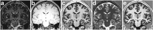
Coronal view of reconstructed images from an MP2RAGE sequence acquired with a 3T Siemens scanner on a subject of the study. The several outputs of the MP2RAGE sequence are (a) , (b) , (c) the bias‐free reconstructed , (d) the map and (e) our phase‐sensitive inversion recovery reconstructed image .
Linear Partial Volume Model
In previous works [Pham and Prince, 1998; Ruan et al., 2000; Santago et al., 1993; Tohka et al., 2004], regardless of the sequence, the signal of a voxel composed of GM and WM has been modeled as a linear combination of intensity means ( and ) of these tissues, assuming no intensity inhomogeneity:
| (3) |
As MP2RAGE provides much reduction of the receiver bias, this linear model seems a good candidate for PVE on the reconstructed image . The model was parameterized by considering the pure tissue means where PV is estimated. The fractional content could thus be computed by interpolating the signal , with constraining the value of in :
| (4) |
where f is defined as
| (5) |
The linear PV model could also be independently applied to or but RF inhomogeneities would be present and the optimized contrasts between cerebral tissues obtained in would not be exploited thus eliminating the advantages of the MP2RAGE sequence.
Bloch‐Based Partial Volume Model
In previous short publications [Duché et al., 2012, 2014], we proposed a new partial volume model to estimate PV from MP2RAGE data. In this model, the parameters contributing to the signal are expressed as the tissue properties and the sequence parameters . The tissue properties are the proton density, the longitudinal relaxation time , the transversal relaxation time T2 and the relaxation time. In MP2RAGE, the sequence parameters can be decomposed in two sets of parameters and corresponding to the two individual acquisitions before combining them with Eq. (1). Hence, the signal measured in a pure tissue voxel is weighted by the longitudinal magnetization of the protons population . Consequently, the two PV signals in and are defined as a linear combination of two pure signals:
| (6) |
where and are the tissue properties of pure GM and WM. values were estimated using the map produced by MP2RAGE, while , and proton density values were assumed constant and taken from the literature [Rooney et al., 2007; Wansapura et al., 1999]. The signal functions and are the MP2RAGE signals measured with the first and second inversion times. More details about these functions can be found in [Marques et al., 2010]. The signals and can then be computed for particular pure tissues, resulting in the estimation of the values . They represent the pure GM and WM signals in and for .
The voxel‐wise linear system [Eq. (6)] can be solved for which are the amounts of respective tissues in the voxel, they represent the same physical information in both MP2RAGE images. Once the signals demodulation is performed, the fractional content of GM is calculated as:
| (7) |
This model is parameterized by the values of tissues. has a limited impact on , as the sequence is strongly weighted [Mugler and Brookeman, 1990].
As the partial volume is estimated from the signal equations, we will later refer to this method as the Bloch model.
Local and Global Models
In our experiments, MPRAGE scans were corrected for bias field using N4 [Tustison et al., 2010], whereas MP2RAGE data were not corrected since the data are natively bias‐free. However, upon close inspection some intensity variations were still noticeable in the corrected MPRAGE and the MP2RAGE images (Fig. 2). Those variations have been reported [Sereno et al., 2013] before as natural contrast variation between GM and WM, and have even been investigated as a possible biomarkers of ageing [Salat et al., 2009]. In addition to estimating one global mean for each tissue as is usually done, we therefore also estimated local tissue intensity.
Figure 2.
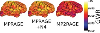
Gray to white matter (GWR) ratios maps computed from MPRAGE, bias‐corrected MRPAGE and MP2RAGE data. These maps were estimated in each voxel of the cortex by computing the ratio between mean gray matter and white matter signals in the neighboring voxels (within a sphere of radius 20 mm) previously classified as GM or WM. [Color figure can be viewed at http://wileyonlinelibrary.com]
In the global approach, the parameters of the PV models (cf., Table 1) were estimated using the pre‐obtained segmentation maps. The GM and WM masks were eroded with a spherical structuring element of radius 1 mm to reduce PV. For the CSF, the ventricles were used and eroded similarly to estimate CSF parameters. The mean intensity values for every tissue inside those masks were used as model parameters for either the linear model (mean intensity in image U) or the Bloch model (T 1 values) and were fixed for every PV voxel in the brain.
Table 1.
Summary of the PV estimation methods
| PV model | Parameters (extracted from) | PV estimated with | ||
|---|---|---|---|---|
| Linear model |
|
|
||
| Bloch model |
|
|
The second column lists the required parameters and the input image(s). The right column lists the image(s) from which the PV estimation is done.
The local method consisted in estimating local pure tissue intensity means for the linear model and local values for the Bloch model (see Table 1). For each PV voxel (see section “Real Brain MR Data at 3T” for the identification of those), a sphere of radius was created. The radius of the sphere was chosen after experimenting with different sizes. It needs to be large enough to be statistically robust but not too large to miss fast spatial variation in intensity. Every voxel labeled as pure tissue inside that sphere contributed to the calculation of the corresponding local pure tissue parameters. maps obtained with MP2RAGE were used to estimate the local values for the Bloch model while images provided the linear model parameters. This local approach allows taking into account the natural variability of the tissue properties across the brain [Salat et al., 2009].
These maps were also used to construct gray‐to‐white matter signal intensity ratios (GWR) at the cortical boundary to compare contrast across sequences. The GWR was utilized in Salat et al. [2009] to reflect the evolution of local GM/WM contrast properties with age.
Simulated Data
In order to compare the various PVE methods, we applied the two PV models on synthetic data that we generated. Two tissues of interest were simulated with different values. PV voxels were simulated by mixing signal with fractional content values , ranging from 0 to 1 by increment of 0.01. The PV signals were modeled as linear combinations of two pure tissue signals. The robustness to noise of the PVE methods was evaluated with a Monte Carlo approach. The two inversion times were simulated with various levels of additive Gaussian noise, approximating Rician noise in tissue, and the composite signals were calculated with Eq. (1). The two PVE methods were applied to estimate the fractional content . For each , the operation was repeated with N = 100.000 samples. For every PVE method and level of noise, the mean and the standard deviation were calculated.
For noiseless simulations, PVE by the various methods was expressed as a function of the ground truth, the PV coefficients . These functions were plotted and compared with the ground truth function . The root mean squared error (RMSE) between the ground truth and the PV estimates was computed.
This simulation was done for six combinations of pair of tissues with the same MP2RAGE imaging parameters. First, the gray‐white and gray‐pial boundaries were simulated with values measured in experimental data of subjects at 3T. The evaluation of the PV estimation errors was extended to brain tissues scanned with MP2RAGE at 7T. values, increasing with the magnetic field strength, were estimated from MP2RAGE maps of the publicly available MRI data set [Forstmann et al., 2014]. In addition, simulations of the PV boundaries obtained in the physical phantom described in the next subsection and scanned at 3T were performed. All the values used for the different magnetic fields and objects are reported in Table 2.
Table 2.
values used for the simulated partial volume GM/WM or GM/CSF voxels
| Simulated tissues |
values at 3T (ms) (brain) |
values at 7T (ms) (brain) |
values at 3T (ms) (physical phantom) |
|---|---|---|---|
| WM | 846 | 1,220 | 316 |
| GM | 1,350 | 2,132 | 504 |
| CSF | 2,900 | 4,425 | 898 |
The acquisition parameters for the 3T simulations were similar to those used for the physical phantom and real data experiments (described in the next subsection): TI1/TI2/TE/TR/ /BW = 700 ms/2,500 ms/2.98 ms/5,000 ms/4°/5°/240 Hz/px. Those for the 7T simulations were TI1/TI2/TE/TR/ /BW = 900 ms/2,750 ms/2.45 ms/5,000 ms/5°/3°/240 Hz/px as in [Forstmann et al., 2014].
Physical Phantom
A physical phantom experiment was designed to compare the PVE methods against a known ground truth.
Design
The phantom consisted of three agar layers. We varied the concentration of gadolinium diethylenetriamine penta‐acetic acid (Gd‐DTPA) in the gels to reproduce the order of values as it may be found in cerebral tissues ( ). The gel layers were designed to be as flat as possible by pouring the hot agar solution onto a flat piece of glass. The three gels were placed on top of each other to obtain a flat interface between neighboring gels. The GM‐like gel was positioned in the bottom followed by the WM‐like gel in the middle and the CSF‐like gel on top.
Imaging Protocol
The phantom was scanned in a 3T Siemens Skyra Scanner with a 20‐channel head coil. A first volume was acquired by placing as precisely as possible the field of view (FOV) coplanar to the flat intersections between gels. This strategy ensures that one slice of the acquired volume (angle 0°) is subject to PV. The FOV was incrementally rotated by an angle until a final FOV angle of 90° was reached. Each FOV position was scanned with a 3D isotropic (1 mm3) MP2RAGE protocol with the following parameters: TI1/TI2/TE/TR/ /BW = 700 ms/2,500 ms/2.98 ms/5,000 ms/4°/5°/240 Hz/px.
Ground Truth Separating Surface Estimation
We made the assumption that locally at the scale of a few pixels, the separating surface between two gels could be approximated with a plane, expressed in the phantom coordinate system. In other words, there exists an optimal plane of equation that represents the interface between two pure tissues. An initial plane was estimated from a manually labeled zone in the first acquired image in a region of the phantom where the PV effects seemed to occur in a single slice. We optimized the plane position by minimizing the root mean squared error (RMSE) between the fractional contents estimated with a PVE method and the computed ground truth:
| (8) |
where is the fractional content ground truth calculated at the voxel index in the region of interest for the current plane position . is the fractional content estimated with the method chosen to minimize the criterion. This procedure was repeated for the linear and Bloch PV models at both interfaces.
Partial Volume Ground Truth Calculation
For every PV voxel, the volume on each side of the intersecting plane surface was geometrically computed from the positions of the intersection points of the current plane and the voxel bounding box. This volume, normalized by the voxel volume, was assigned to the corresponding tissue PV map. PV was estimated on voxels identified as PV voxels during the ground truth calculation step. The parameters for the PVE methods were measured with manually labeled regions for each of the three tissues.
Real Brain MR Data at 3T
Six healthy volunteers were scanned in a 3T Siemens Skyra scanner with a 20‐channel head coil (Siemens, Erlangen Germany), at Monash University, Melbourne, Australia, under ethics approval of the Monash University Human Research Ethics Committee (MUHREC). Each subject was scanned with a 3D isotropic (1 mm3) MP2RAGE protocol (the parameters were similar to those used in the physical phantom experiment, the resulting MP2RAGE images are shown in Fig. 1) and a 3D isotropic MPRAGE protocol with the following parameters: . The subject was scanned a first time (scan) with both sequences, and then was asked to stand up before acquiring another pair of images (rescan). The subject had therefore two different head positions between the two scanning sessions.
Each subject was processed with the following pipeline. The four volumes (MP2RAGE scan and rescan and MPRAGE scan and rescan) were coregistered to a common coordinate system thus allowing to compute an average volume. This volume was segmented into five classes: CSF, CSF/GM, GM, GM/WM, and WM as detailed in Acosta et al. [2009]. The obtained mask was projected backward in the original space of each volume with the inverse transforms calculated during the previous step. GM PV maps were obtained by applying the PV models presented earlier: Partial Volume Models subsection the linear and Bloch PV models for the MP2RAGE volumes and the linear model for the MPRAGE volumes.
These PV maps were either obtained using global pure tissue intensity means or local pure tissue intensity means as described in the Methods section.
The influence of PVE on cortical thickness measurements was assessed. Cortical thickness was estimated with a voxel‐based method [Acosta et al., 2009] that requires a GM/WM/CSF segmentation and a GM PV map as inputs. The cortical thickness maps associated to each PVE method were computed with a common segmentation and the three different estimated GM PV maps.
For each scan, three cortical thickness maps were estimated. Hence, six cortical thickness maps were obtained per subject. They were aligned on a common template surface to compare the results on a vertex‐wise basis. The average cortical thickness in the whole neocortex was computed and compared between PV models.
The topologically equivalent surfaces allowed vertex‐wise comparisons. We computed the mean cortical thickness difference between all the pair of PV models among the 12 images (6 subjects × 2 scans). Reproducibility of cortical thickness measurement was estimated by computing the correlation coefficient for vertex‐wise cortical thickness values between the first and the second scans.
A vertex‐wise statistical analysis was performed in order to compare PV models. The cortical thickness of individual at vertex for the scan number was modeled with the following linear mixed effects model similar as the one presented in Ospina et al. [2012]:
| (9) |
where, is the average cortical thickness of the population at vertex , is the average cortical thickness difference between two PV models at vertex , is 0 if was estimated with the linear model and 1 otherwise ( was estimated with the Bloch model), is the deviation of individual from the population and is a random error related to scan number . The statistical test consisted in testing the following null hypothesis: . If the null hypothesis was not rejected, there was no evidence of differences in between the cortical thickness estimated from the two different PV models. If the null hypothesis was rejected, PV models were said to induce statistically significant differences in the estimation of cortical thickness. The vertices with significant difference between the two metrics were displayed on our template surface.
RESULTS
Local and Global Models
Figure 2 shows gray to white matter signal intensity ratios (GWR) at each vertex of a cortical surface reconstructed from MPRAGE and MP2RAGE data, showing consistent results as those reported by Salat et al. [2009]. MP2RAGE had superior tissue contrast compared with MPRAGE. The average GWR over the surface for the subject shown in Figure 1 was 0.68 for MP2RAGE data and 0.78 for MPRAGE data. Figure 2 also highlights that GWR contrast varies throughout the cortex, even in MPRAGE after correction with N4. It shows that the GWR variation patterns across the brain were similar between MPRAGE (with and without N4 bias correction) and MP2RAGE (no bias correction); however, the amplitude of the variations was different.
Simulated Data
The sensitivity to noise on the estimate of the coefficients with the two PVE methods on MP2RAGE simulated data appeared to vary linearly with noise level. The linear relationship was the same for the linear and Bloch models. While the Bloch model did not exhibit bias in the PV coefficients estimation, the linear model resulted in systematic errors for any pair of tissues considered in the simulations when applied on the uniform MP2RAGE image. The shape of the error function varies with the pair of tissues considered for partial volume correction (Fig. 3). The theoretical error is a function of the tissue properties; therefore, the trend of the error function varies with the magnetic field strength.
Figure 3.
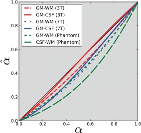
Estimated partial volume coefficients ( ) versus ground truth coefficients ( ) with simulated MP2RAGE signals using the linear PV model for various tissue boundaries and magnetic field strengths. [Color figure can be viewed at http://wileyonlinelibrary.com]
We also investigated the effect of higher field strength (7T). At 3T, depending on the actual GM PV coefficient, positive or negative low magnitude ( ) PV errors occur at the GM/CSF boundary and negative errors occur at the GM/WM boundary. At 7T, the errors are consistently negative: the linear model underestimates the proportion of GM at both boundaries, the errors at 7T were larger than those at 3T.
Physical Phantom
The values of the phantom measured with the MP2RAGE map were of 504 ms for the GM‐like gel, 316 ms for the WM‐like and 898 ms for the CSF‐like, and although these values were not identical to cerebral tissue properties measured at 3T (due to experimental constraints), the gels reproduce values in the same order as it may be found in cerebral tissues ( ). Figure 4 (top) shows three regions of interest obtained in MP2RAGE uniform images acquired with various FOV inclination angles. The acquisition strategy resulted in a uniform sampling of the PV coefficients as the patterns observable at interfaces vary between images. Intensity profiles were drawn from these images and were plotted in Figure 4 (bottom).
Figure 4.
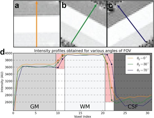
Example of the images for varying slice inclination angles (panels a, b, c) for the physical phantom using the MP2RAGE sequence. The corresponding signal profiles are plotted below for the various inclination angles (panel d). In the graph, the points overlaid with a red box are signals coming from PV voxels, reflecting the variety of PV coefficients obtained with this scanning scheme. [Color figure can be viewed at http://wileyonlinelibrary.com]
The optimized plane positions obtained for each PV model were very similar, validating that both models estimated a common optimal plane solution. Indeed, the normal coefficients differed by less than 0.1% between the linear and Bloch PV models and the elevation of the plane differed by only 0.02 mm. RMSE obtained by minimizing the criterion with the linear model (0.21) was higher than the Bloch model (0.12) for the WM/CSF boundary, consistent with the hypothesis that the linear model is subject to both statistical and systematic errors while the Bloch model may be subject to the noise contribution only.
The scatter plots of PV voxels obtained at both boundaries are shown in Figure 5 (top: WM/CSF, bottom: GM/WM). The x‐axis is the PV ground truth obtained for the optimal plane position while the y‐axis is the PV estimated with the PV model used for optimization. These plots show a bias for the linear model at the WM/CSF boundary, consistent with our simulation results, and well fitted with a second degree polynomial as predicted from simulations.
Figure 5.
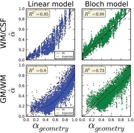
PV coefficients in PV voxels at the interface of the gel layers. The data were concatenated from every inclination angle of the field of view. In blue, the scatter plots obtained for the linear model and in green for the Bloch model. The scatter plots represent the estimated PV coefficients versus the estimated geometrical ground truth ( ) obtained with the optimal plane position model. Top row: PV voxels belonging to the phantom WM/CSF boundary. Bottom row: PV voxels belonging to the phantom GM/WM boundary. For each boundary, the solutions obtained for the linear and Bloch models were very close; however, the blue points (linear model) follow a quadratic function of the ground truth PV coefficients while the green points (Bloch model) follow a linear relationship with the ground truth PV coefficients. [Color figure can be viewed at http://wileyonlinelibrary.com]
Real Brain MR Data at 3T
The results of the comparisons between PV models and sequences with the local PV approach are summarized in Figure 6. The top row contains the cumulated histograms of cortical thickness differences across the population and the bottom row exhibits surfaces where the vertices code for the p‐value calculated from the linear mixed effects model presented in Eq. (9).
Figure 6.
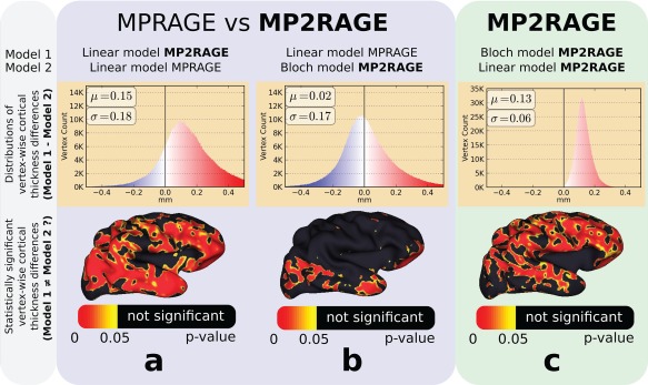
Cortical thickness results using a local intensity estimation from three PV models and sequences compared (three columns of panels). The histograms plots (upper panels) show the vertex‐wise cortical thickness difference distributions. The bottom row of panels is meshes representing statistically significant cortical thickness differences that are due to the models. The bias seen in the left column using MPRAGE and MP2RAGE with the standard linear model can be removed using our proposed approach for MP2RAGE (middle column). A similar bias is seen in the right column between the linear and our proposed “Bloch model” using MP2RAGE, with a narrower error distribution since no registration was necessary as the same image was used (MP2RAGE) for both methods. [Color figure can be viewed at http://wileyonlinelibrary.com]
The average cortical thickness difference between the Bloch and linear models with MP2RAGE data was 0.13 mm for the local model (0.09 mm for the global model), shown in the histograms in the Figure 6 upper row, rightmost column. Between the Bloch model (MP2RAGE) and the linear model applied on MPRAGE the difference was 0.02 mm for the local model (–0.10 mm for the global model). The reproducibility was similar between PV models and sequences with an average of 0.799, 0.796, and 0.812 for the linear model applied on MPRAGE, the linear model applied on M2PRAGE and the Bloch model (MP2RAGE), respectively.
The p‐value surfaces show a large number of vertices with statistically significant differences between the linear and Bloch PV models on MP2RAGE and between the linear model applied on MP2RAGE and on MPRAGE throughout the whole brain surface (Fig. 6, bottom). However, fewer vertices had statistically significant differences between the linear model applied on MPRAGE data and the Bloch PV model (MP2RAGE data), and were localized in the temporal lobe and bottom of the frontal lobe.
values as measured by MP2RAGE shows variability across the brain (Fig. 7). Using local tissue intensity means instead of global tissue average allowed to take into account this natural tissue variability resulting in differences of cortical thickness (Fig. 8).
Figure 7.
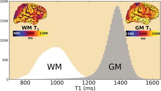
Distribution of estimated values of cortical GM and neighboring WM voxels at 3T for the whole population. The pictures in the corners of the graph show the WM and GM surface projection for a representative subject. [Color figure can be viewed at http://wileyonlinelibrary.com]
Figure 8.
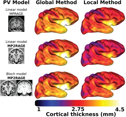
Average cortical thickness surfaces obtained from the six subjects using either the local or global model and the various PV models are represented line‐wise. [Color figure can be viewed at http://wileyonlinelibrary.com]
DISCUSSION
Partial volume estimation using a linear mixed model often used with MPRAGE is not valid for MP2RAGE acquisition because the composite image introduces a quadratic component. Instead, a Bloch‐based PV model was proposed to take into account this quadratic term. Using a linear PV model on MP2RAGE results in the underestimation of cortical thickness as reported by others [Fujimoto et al., 2014]. This error could be corrected in our experiments when using the Bloch model on MP2RAGE data. There are two features in using the proposed PV model: it is based on the Bloch equations (it allows to model the sequence parameters) and it is based on the and images prior to any non‐linear combination (the source of the thickness bias compared with MPRAGE). This last feature allows correcting partial volume estimation in MP2RAGE volumes. We demonstrated those findings on (i) simulations, (ii) physical phantom, and in (iii) a reproducibility study on six subjects. In addition, contrast between white and gray matter is not constant across the brain, and can be measured with MP2RAGE map variation. We suggest using partial volume models that include local estimate of tissue intensity to take into account this natural variation, rather than estimating a single intensity mean for each tissue.
Our simulations suggest (Fig. 3) that the measured error functions depend on the pair of tissues considered. These functions vary with the magnetic field strength and they vary unfavorably for the linear PV model when magnetic field strength increases. The GM/CSF boundary at 3T has relatively small errors when comparing to ground truth (plain red line in Fig. 3) and would have limited impact on CTE. The 7T simulations suggest that the errors are more significant (blue lines, Fig. 3), resulting in a systematic underestimation of the GM volume. These errors cumulated on both sides of the cortex may result in a consistently underestimated cortex from MP2RAGE compared with MPRAGE when using a classic linear PV model. The achievable higher resolution at 7T would only partially reduce the influence of these errors. However, investigation of those issues at 7T remains to be done.
The physical phantom experiment validated the simulation results with a good fit between the expected error and the measured error for the linear PV model at the WM/CSF boundary. The experimental results for the GM/WM boundary had a slight shift compared with our theoretical model. We believe that the lower interface between the gels was probably not ideally flat challenging our ideal plane model. Gibbs oscillations visible in Figure 4 probably affected also our PV measurements.
Our findings explain the systematic measurements of a thinner cortex reconstructed with MP2RAGE compared with a cortex reconstructed with the reference multi‐echo MPRAGE (MEMPRAGE) scan reported in Fujimoto et al. [2014]. The authors reported an average cortical thickness difference of 0.12 mm between the cortical surfaces reconstructed from MEMPRAGE scans and MP2RAGE. This difference is consistent with the one observed between the linear and Bloch PV models in our cortical thickness measurements (average 0.13 mm). Using a physical phantom, the errors in PV estimation were consistent and only slightly larger than the theoretical errors, probably due to the errors in calculating a precise PV ground truth. However, a similar quadratic trend was observed, confirming that the linear model is prone to PV errors at both interfaces of the GM. Even though they can be low, they are systematic and introduce a bias in the estimation, which can be avoided by choosing the Bloch PV model for MP2RAGE. Fujimoto et al. performed a vertex analysis comparison of the reconstructed surfaces suggesting that the MP2RAGE gray‐white boundary was responsible for most of the discrepancies between MEMPRAGE and MP2RAGE. This analysis is consistent with our results showing that the PVE bias with the linear model is larger at the gray‐white boundary than at the pial surface for a magnetic field strength of 3T.
The cortical thickness results in Fujimoto et al. [2014] were obtained with a surface‐based approach step [Dale et al., 1999] whereas our results come from a voxel‐based method. While the two approaches are different, they share the same assumption that an intensity edge defines the GM/WM boundary. This boundary is shifted when using a linear model in the MP2RAGE image. This is consistent with comparison between surface‐based and voxel‐based approaches in population analysis. Acosta et al. [2012] have reported a high correlation in cortical thickness estimated with both voxel‐based approach and the surface‐based approach obtained by Freesurfer. This appears to be in agreement with results from Clarkson et al. [2011] that for group‐wise comparisons, surface and voxel‐based methods produce comparable results.
The linear PV model could be applied independently to , or to , but by doing so, the bias‐free and high GM/WM contrast features of the combined MP2RAGE image would not be exploited. However, while values are measured with MP2RAGE, the unknown proton density values of the tissues have to be estimated, which is a limitation of our approach. Our proposed Bloch model allows to take into account the actual flip angle which could vary from the desired flip angle with inhomogeneities at high field. This effect could be reduced if flip angle mapping could be performed. We expect that the Bloch model would benefit from the more recent MP3RAGE sequence [Rioux et al., 2014] that allows both and flip angle measurement.
We did not find any difference in reproducibility between the models and sequences tested. This is likely due to our careful experimental design to fairly compare the methods. Using identical segmentation maps for both MPRAGE and MP2RAGE (calculated on the average image) PV voxels were labeled in the same way for all the images. The alternative method of independently segmenting images from each sequence and model creates different PV labels, which in our experiments produced different cortical thickness reproducibility results that could not be fully attributed to the chosen PV model (since the source of the errors could also come from the different segmentations).
No bias field correction in a pre‐processing step is required before segmenting MP2RAGE scans since it is free of the RF B1 inhomogeneity. However, close inspection of reconstructed MP2RAGE and volumes shows signal intensity variations across the brain. MRI intensity variation across the brain is present naturally as tissue microstructure and properties affect each voxel's magnetic and relaxation properties. This was recognized and shown to be independent of the MRI system and sequences [Salat et al., 2009]. In fact, not only GM, but also the WM signal intensity varies across the brain due to different tissue properties (cf., Fig. 7), resulting in GM/WM contrast variation. Figure 2 illustrates the local variations of the GM to WM signal ratio with MPRAGE and MP2RAGE acquired on the same healthy subject. Figure 8 shows cortical thickness differences between the PV models; it also shows differences between global and local methods albeit more subtle because of the color map used. Using local averages leads to better estimation of PV for estimating cortical thickness in MPRAGE [Rueda et al., 2010], and we expect this to be the case for MP2RAGE as well as suggested by Figure 8. The low frequency of the RF bias field overlaps the smooth intensity variation of the tissue, and thus applying methods like N4, which enforces constant tissue intensity across the brain, results in a decrease of potentially useful information. However, as shown in Figure 2, tissue intensity can vary quickly between areas and some of the natural tissue variation remains even after N4 pre‐processing of MPRAGE (Fig. 2 middle panel). Because MP2RAGE does not require bias field correction, the variation intensity of the tissues across the brain are likely to be due solely to the natural intensity variation, and are larger than in MPRAGE as computed by the grey to white intensity ratio (Fig. 2). This makes MP2RAGE an ideal candidate to investigate the utility of the intensity variation across brain tissues as a biomarker of pathologies or ageing, which will be the focus of our future work.
CONCLUSION
We investigated different PV models to estimate the fractional tissue contents in brain MRI with the MP2RAGE sequence. We showed that the well‐established linear model for PVE is prone to systematic errors because the reconstructed MP2RAGE image results from a non‐linear (quadratic) combination of two images. Instead, we demonstrated and validated the use of a Bloch‐based PV model on phantom and actual 3T brain data. Furthermore, tissue intensities vary across the brain, and the assumption of a constant tissue mean intensity is not valid. We suggest using a local estimate of tissue intensity. By using a forward model based on the Bloch equations with local tissue intensity estimate, similar cortical thickness estimation could be achieved between MP2RAGE and the standard linear method applied to MPRAGE. This suggests that MP2RAGE when processed with a tailored PV model is an excellent candidate for brain morphometry and should be considered for future clinical studies. More studies are however warranted to investigate its value in larger cohorts and for biomarker computation in brain disorders.
ACKNOWLEDGMENTS
We would like to thank Juan David Ospina from the Universidad Nacional de Colombia for his help and feedback on data analysis.
Contributor Information
Oscar Acosta, Email: oscar.acosta@univ-rennes1.fr.
Olivier Salvado, Email: olivier.salvado@csiro.au.
REFERENCES
- Acosta O, Bourgeat P, F Jurgen, B Erik, O Sébastien, S Olivier (2008): Automatic delineation of sulci and improved partial volume classification for accurate 3d voxel‐based cortical thickness estimation from MR. Med Image Comput Comput Assist Interv 2008;11:253–261. [DOI] [PubMed] [Google Scholar]
- Acosta O, Bourgeat P, Zuluaga MA, Fripp J, Salvado O, Ourselin S (2009): Automated voxel‐based 3d cortical thickness measurement in a combined lagrangian‐eulerian pde approach using partial volume maps. Med Image Anal 13:730–743. [DOI] [PMC free article] [PubMed] [Google Scholar]
- Acosta O, Fripp J, Doré V, Bourgeat P, Favreau J‐M, Chatelat G, Rueda A, Villemagne VL, Szoeke C, Ames D, Ellis KA, Martins RN, Masters CL, Rowe CC, Bonner E, Gris F, Xiao D, Raniga P, Barra V, Salvado O (2012): Cortical surface mapping using topology correction, partial flattening and 3d shape context‐based non‐rigid registration for use in quantifying atrophy in alzheimer's disease. J Neurosci Methods 205:96–109. [DOI] [PubMed] [Google Scholar]
- Ashburner J, Friston K (1997): Multimodal image coregistration and partitioning—a unified framework. NeuroImage 6:209–217. [DOI] [PubMed] [Google Scholar]
- Ashburner J, Friston KJ (2005): Unified segmentation. NeuroImage 26:839–851. [DOI] [PubMed] [Google Scholar]
- Bazin PL, Weiss M, Dinse J, Schäfer A, Trampel R, Turner R (2013): A computational framework for ultra‐high resolution cortical segmentation at 7 tesla. NeuroImage 93:201–209. [DOI] [PubMed] [Google Scholar]
- Bourgeat P, Acosta O, Zuluaga M, Fripp J, Salvado O, Ourselin S (2008): Improved cortical thickness measurement from mr images using partial volume estimation. In: 2008 5th IEEE International Symposium on Biomedical Imaging: From Nano to Macro, 205–208.
- Brouwer RM, Hulshoff Pol HE, Schnack HG (2010): Segmentation of MRI brain scans using non‐uniform partial volume densities. NeuroImage 49:467–477. [DOI] [PubMed] [Google Scholar]
- Choi HS, Haynor DR, Kim Y (1991): Partial volume tissue classification of multichannel magnetic resonance images‐a mixel model. IEEE Trans Med Imaging 10:395–407. [DOI] [PubMed] [Google Scholar]
- Clarkson MJ, Cardoso MJ, Ridgway GR, Modat M, Leung KK, Rohrer JD, Fox NC, Ourselin S (2011): A comparison of voxel and surface based cortical thickness estimation methods. NeuroImage 57:856–865. [DOI] [PubMed] [Google Scholar]
- Dale AM, Fischl B, Sereno MI (1999): Cortical surface‐based analysis. NeuroImage 9:179–194. [DOI] [PubMed] [Google Scholar]
- Doré V, Villemagne VL, Bourgeat P, Fripp J, Acosta O, Chetélat G, Zhou L, Martins R, Ellis KA, Masters CL, Ames D, Salvado O, Rowe CC (2013): Cross‐sectional and longitudinal analysis of the relationship between aβ deposition, cortical thickness, and memory in cognitively unimpaired individuals and in alzheimer disease. JAMA Neurol 70:903. [DOI] [PubMed] [Google Scholar]
- Duché Q, Acosta O, Gambarota G, Merlet I, Salvado O, Saint‐Jalmes H (2012): Bi‐exponential magnetic resonance signal model for partial volume computation. Med Image Comput Comput Assist Interv 2012;15:231–238. [DOI] [PMC free article] [PubMed] [Google Scholar]
- Duché Q, Raniga P, Egan GF, Acosta O, Gambarota G, Salvado O, Saint‐Jalmes H (2014): New partial volume estimation methods for MRI MP2RAGE. Med Image Comput Comput Assist Interv 2014;17:129–136. [DOI] [PubMed] [Google Scholar]
- Fischl B, Sereno MI, Dale AM (1999): Cortical surface‐based analysis. NeuroImage 9:195–207. [DOI] [PubMed] [Google Scholar]
- Forstmann BU, Keuken MC, Schafer A, Bazin P‐L, Alkemade A, Turner R (2014): Multi‐modal ultra‐high resolution structural 7‐tesla mri data repository. Sci Data 1:140050. [DOI] [PMC free article] [PubMed] [Google Scholar]
- Fujimoto K, Polimeni JR, van der Kouwe AJW, Reuter M, Kober T, Benner T, Fischl B, Wald LL (2014): Quantitative comparison of cortical surface reconstructions from mp2rage and multi‐echo mprage data at 3 and 7T. NeuroImage 90:60–73. [DOI] [PMC free article] [PubMed] [Google Scholar]
- Gonzalez Ballester MA, Zisserman AP, Brady M (2002): Estimation of the partial volume effect in MRI. Med Image Anal 6:389–405. [DOI] [PubMed] [Google Scholar]
- Jack CR, Bernstein MA, Fox NC, Thompson P, Alexander G, Harvey D, Borowski B, Britson PJ, Whitwell JL, Ward C, Dale AM, Felmlee JP, Gunter JL, Hill DLG, Killiany R, Schuff N, Fox-Bosetti S, Lin C, Studholme C, DeCarli C.S., Krueger G, Ward HA, Metzger GJ, Scott KT, Mallozzi R, Blezek D, Levy J, Debbins JP, Fleisher AS, Albert M, Green R, Bartzokis G, Glover G, Mugler J, Weiner MW, ADNI Study (2008): The Alzheimer's disease neuroimaging initiative (adni): mri methods. J Magn Reson Imaging 27:685–691. [DOI] [PMC free article] [PubMed] [Google Scholar]
- Khademi A, Venetsanopoulos A, Moody AR (2014): Generalized method for partial volume estimation and tissue segmentation in cerebral magnetic resonance images. J Med Imaging 1:014002. [DOI] [PMC free article] [PubMed] [Google Scholar]
- Leemput KV, Maes F, Vandermeulen D, Suetens P (1999a): Automated model‐based bias field correction of mr images of the brain. IEEE Trans Med Imaging 18:885–896. [DOI] [PubMed] [Google Scholar]
- Leemput KV, Maes F, Vandermeulen D, Suetens P ( 1999b): Automated model‐based tissue classification of mr images of the brain. IEEE Trans Med Imaging 18(10):897–908. [DOI] [PubMed] [Google Scholar]
- Marques JP, Kober T, Krueger G, van der Zwaag W, Van de Moortele P‐F, Gruetter R (2010): MP2RAGE, a self bias‐field corrected sequence for improved segmentation and t1‐mapping at high field. NeuroImage 49:1271–1281. [DOI] [PubMed] [Google Scholar]
- Mugler JP, Brookeman JR (1990): Three‐dimensional magnetization‐prepared rapid gradient‐echo imaging (3D MP RAGE). Magn Reson Med 15:152–157. [DOI] [PubMed] [Google Scholar]
- Ospina JD, Acosta O, Crevoisier R, Correa JC, Haigron P (2012): A non parametric mixed‐effect model for population analysis: Application to alzheimer's disease data. In: 2012 9th IEEE International Symposium on Biomedical Imaging (ISBI). pp 1124–1127.
- Pham DL, Prince JI (1998): Partial volume estimation and the fuzzy c‐means algorithm [brain mri application]. In: Proceedings 1998 International Conference on Image Processing. ICIP98 (Cat. No.98CB36269). pp 819–822. [Google Scholar]
- Rioux JA, Saranathan M, Rutt BK (2014): Simultaneous whole‐brain t1 and flip angle mapping with MP3RAGE. In: ISMRM.
- Rooney WD, Johnson G, Li X, Cohen ER, Kim S, Ugurbil K, Springer CS ( 2007): Magnetic field and tissue dependencies of human brain longitudinal 1h2o relaxation in vivo. Magn Reson Med 57:308–318. [DOI] [PubMed] [Google Scholar]
- Ruan S, Jaggi C, Xue J, Fadili J, Bloyet D (2000): Brain tissue classification of magnetic resonance images using partial volume modeling. IEEE Trans Med Imaging 19:1179–1187. [DOI] [PubMed] [Google Scholar]
- Rueda A, Acosta O, Couprie M, Bourgeat P, Fripp J, Dowson N, Romero E, Salvado O (2010): Topology‐corrected segmentation and local intensity estimates for improved partial volume classification of brain cortex in MRI. J Neurosci Methods 188:305–315. [DOI] [PubMed] [Google Scholar]
- Salat DH, Lee SY, van der Kouwe AJ, Greve DN, Fischl B, Rosas HD (2009): Age‐associated alterations in cortical gray and white matter signal intensity and gray to white matter contrast. NeuroImage 48:21–28. [DOI] [PMC free article] [PubMed] [Google Scholar]
- Santago P, Donald Gage H, Member S (1993): Quantification of MR brain images by mixture density and partial volume modeling. Development 12:566–574. [DOI] [PubMed] [Google Scholar]
- Sereno MI, Lutti A, Weiskopf N, Dick F (2013): Mapping the human cortical surface by combining quantitative T1 with retinotopy. Cereb Cortex 23:2261–2268. [DOI] [PMC free article] [PubMed] [Google Scholar]
- Shattuck DW, Sandor‐Leahy SR, Schaper KA, Rottenberg DA, Leahy RM (2001): Magnetic resonance image tissue classification using a partial volume model. NeuroImage 13:856–876. [DOI] [PubMed] [Google Scholar]
- Smith SM, Jenkinson M, Woolrich MW, Beckmann CF, Behrens TEJ, Johansen‐Berg H, Bannister PR, De Luca M, Drobnjak I, Flitney DE, Niazy RK, Saunders J, Vickers J, Zhang Y, De Stefano N, Brady JM, Matthews PM (2004): Advances in functional and structural mr image analysis and implementation as FSL. NeuroImage 23:S208–S219. [DOI] [PubMed] [Google Scholar]
- Tohka J, Zijdenbos A, Evans A (2004): Fast and robust parameter estimation for statistical partial volume model in MRI. NeuroImage 23:84–97. [DOI] [PubMed] [Google Scholar]
- Tustison NJ, Avants BB, Cook PA, Zheng Y, Egan A, Yushkevich PA, Gee JC (2010): N4ITK: Improved N3 bias correction. IEEE Trans Med Imaging 29:1310–1320. [DOI] [PMC free article] [PubMed] [Google Scholar]
- Van Leemput K, Maes F, Vandermeulen D, Suetens P (2003): A unifying framework for partial volume segmentation of brain mr images. IEEE Trans Med Imaging 22:105–119. [DOI] [PubMed] [Google Scholar]
- Wansapura JP, Holland SK, Dunn RS, Ball WS (1999): NMR relaxation times in the human brain at 3.0 Tesla. J Magn Reson Imaging 9:531–538. [DOI] [PubMed] [Google Scholar]
- Zhang Y, Brady M, Smith S (2001): Segmentation of brain mr images through a hidden markov random field model and the expectation‐maximization algorithm. IEEE Trans Med Imaging 20:45–57. [DOI] [PubMed] [Google Scholar]
- Zuluaga MA, Acosta O, Bourgeat P, Hoyos MH, Salvado O, Ourselin S (2008): Cortical thickness measurement from magnetic resonance images using partial volume estimation. In: Proceedings on SPIE 6914, Medical Imaging 2008. p 69140J.