MICA—A toolbox for masked independent component analysis of fMRI data

Abstract

Independent component analysis (ICA) is a widely used technique for investigating functional connectivity (fc) in functional magnetic resonance imaging data. Masked independent component analysis (mICA), that is, ICA restricted to a defined region of interest, has been shown to detect local fc networks in particular brain regions, including the cerebellum, brainstem, posterior cingulate cortex, operculo‐insular cortex, hippocampus, and spinal cord. Here, we present the mICA toolbox, an open‐source GUI toolbox based on FSL command line tools that performs mICA and related analyses in an integrated way. Functions include automated mask generation from atlases, essential preprocessing, mICA‐based parcellation, back‐reconstruction of whole‐brain fc networks from local ones, and reproducibility analysis. Automated slice‐wise calculation and cropping are additional functions that reduce computational time and memory requirements for large analyses. To validate our toolbox, we tested these different functions on the cerebellum, hippocampus, and brainstem, using resting‐state and task‐based data from the Human Connectome Project. In the cerebellum, mICA detected six local networks together with their whole‐brain counterparts, closely replicating previous results. MICA‐based parcellation of the hippocampus showed a longitudinally discrete configuration with greater heterogeneity in the anterior hippocampus, consistent with animal and human literature. Finally, brainstem mICA detected motor and sensory nuclei involved in the motor task of tongue movement, thereby replicating and extending earlier results. Hum Brain Mapp 37:3544–3556, 2016. © 2016 Wiley Periodicals, Inc.

INTRODUCTION

Independent component analysis (ICA) is a widely used technique for investigating functional magnetic resonance imaging (fMRI) data [McKeown et al., 1998]. The most frequently used approach, spatial ICA, decomposes the BOLD signal into spatially independent components (ICs), where each IC consists of voxels that show similar signal fluctuations (temporal coherence). One advantage of ICA over conventional techniques based on the general linear model (GLM) is a capacity to detect temporal activation patterns and spatial connectivity networks, without the need for an a priori model of the expected BOLD signal. This makes ICA a suitable technique for exploratory analysis of resting‐state functional magnetic resonance imaging (rfMRI) data, where it is frequently used to study functional connectivity networks, like the default mode network (DMN) [Beckmann et al., 2005; Raichle et al., 2001]. Functional connectivity, including resting‐state connectivity, shows good correspondence with underlying neural circuits and anatomical connections [Baria et al., 2013; Damoiseaux and Greicius, 2009], and has been utilized in a variety of analytical methods to parcellate brain structures into subregions [Bzdok et al., 2013; Chase et al., 2015; Kim et al., 2010; Rebola et al., 2012; Shen et al., 2010].

The way ICA is commonly applied to detect functional connectivity (i.e., using a rather low number of dimensions) is optimized for detecting large‐scale networks [Ray et al., 2013] and, therefore, not optimized to study regional networks, especially in smaller brain structures, like the cerebellum [Dobromyslin et al., 2012], or the brainstem [Beissner et al., 2011]. Masked independent component analysis (mICA), that is, an ICA in a defined region of interest, is a technique recently used by several groups to study such local connectivity networks. It has been referred to by various terms, including spatially restricted ICA [Leech et al., 2012], localized ICA [Sohn et al., 2012], or mICA [Beissner et al., 2014]. To date, mICA has been successfully applied to study many different regions, including the cerebellum, brainstem, primary motor cortex, hippocampus, and spinal cord [Beissner et al., 2014; Blessing et al., 2016; Dobromyslin et al., 2012; Igelström et al., 2015; Kong et al., 2014; Rebola et al., 2012; Sohn et al., 2012]. In these studies, mICA was mostly used to map subregional connectivity networks or parcellate anatomical structures into functionally‐defined subregions.

Once detected, local connectivity networks (i.e., mICs) can be back‐projected to the whole brain or any other brain region, resulting in region‐to‐whole‐brain or region‐to‐region functional connectivity [Beissner et al., 2014]. We will refer to this connectivity henceforth as “global,” as it is located outside the mask used in the original ICA. Several methods have been applied to derive global connectivity networks. the dual‐regression approach [Filippini et al., 2009; Zuo et al., 2010] was used by Leech et al. to derive whole‐brain connectivity of local networks detected in the posterior cingulate cortex [Leech et al., 2012]. Another method for investigating global connectivity is direct back‐reconstruction [Calhoun et al., 2001]. This approach has been applied in conjunction with mICA to derive global connectivity of cerebellar [Dobromyslin et al., 2012] and brainstem networks [Beissner et al., 2014].

Here, we present the mICA toolbox (http://www.nitrc.org/projects/mica/), an open‐source GUI toolbox that performs mICA and related analyses, including automated generation of masks from atlases, estimation of global connectivity, generation of mICA‐based parcellations, and assessment of reproducibility. It also offers an alternative approach to dimensionality estimation. ICA approaches are in general unable to determine the number of components, that is, the decomposition dimensionality [Beckmann and Smith, 2004]; thus, this step is usually achieved empirically, or using information‐theoretic approaches [Beckmann and Smith, 2004; Li et al., 2007]. However, performing ICA with a suboptimal number of components can result in either under‐ or over‐fitting of the data, both of which can seriously affect interpretation of the results. Since this problem is particularly an issue when exploring local connectivity networks with mICA (because different brain regions may have different numbers of local networks), the mICA toolbox offers an alternative approach to dimensionality estimation. It constrains the dimensionality parameter by choosing that which maximizes reproducibility of the results. To this end, the toolbox calculates the reproducibility of mICA results for a range of dimensionality values using repetitive random split‐half sampling or test‐retest analyses.

The mICA toolbox is purely based on command line tools from the FSL suite [Jenkinson et al., 2012]; no new algorithms are introduced. However, functions like atlas‐based mask generation, back‐reconstruction from masked region to whole brain, and reproducibility analysis usually require extensive scripting and/or frequent manual intervention, whereas our toolbox makes them easily accessible by means of a graphical user interface (GUI). Furthermore, built‐in functions reduce computational time and memory requirements for large analyses by automatically cropping the data to the minimum volume containing the mask, and by computing GLMs of back‐reconstruction analyses in a slice‐by‐slice fashion.

Here, we demonstrate the functionality of the mICA toolbox by utilizing it to perform various mICA analyses on three different brain regions. For the cerebellum, we derived local connectivity networks, which were then used for parcellation, and reconstruction of associated global networks. For the hippocampus, we assessed reproducibility of group‐level mICA‐based parcellation on the single‐subject level. For the brainstem, we showed detection of specific motor and sensory nuclei in a motor task involving tongue movement.

MATERIALS AND METHODS

License, Source, and Underlying Software

The mICA toolbox is free and open source software released under the GNU General Public License. It can be obtained from http://www.nitrc.org/projects/mica/. The toolbox is based on the FSL analysis suite (http://fsl.fmrib.ox.ac.uk) and includes functions performed by calling bash scripts which in turn use command‐line tools from FSL, namely, MELODIC, FSL_GLM, MM, FSLUTILS (fslmaths, fslslice, fslmerge, etc.), and dual regression [Beckmann and Filippini, 2009; Jenkinson et al., 2012; Smith et al., 2004; Woolrich et al., 2009]. Probabilistic atlases that come with the FSL package are also used in the toolbox to generate masks of brain regions. The GUI of the toolbox is written in TCL (Tool Command Language, http://www.tcl.tk) and can be executed on Linux or Mac operating systems after installing FSL. The reproducibility module of the toolbox additionally requires Python (http://www.python.org) and the package “munkres” (http://software.clapper.org/munkres/), which contains an implementation of the Hungarian sorting algorithm [Munkres, 1957]. The toolbox and all of its requirements are open‐source software and free of charge.

Functionality and Workflow of mICA Toolbox

The main view of the toolbox provides the user with a simple interface that covers the following main functionalities: single‐session/group mICA, mask generation from atlas, back‐reconstruction and reproducibility analysis (Fig. 1).

Figure 1.

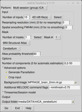
The graphical user interface of the mICA toolbox. [Color figure can be viewed in the online issue, which is available at http://wileyonlinelibrary.com.]

Data preprocessing should comprise the usual steps, like distortion/motion correction, high‐pass filtering, and spatial normalization to standard space. While the input fMRI data should ideally be preprocessed before being used with mICA toolbox, a number of preprocessing steps, such as smoothing, resampling and cropping can be applied using the toolbox itself. The motivation to apply these operations using the toolbox is that they will be applied in an optimal order to achieve good mICA results [Beissner, 2015]. It is important to mask input fMRI data before applying any spatial smoothing, as this approach prevents signal from voxels outside of the mask influencing the signal of those inside. Cropping of input images to the mask's field‐of‐view allows faster reading of input files, thereby speeding up analysis (especially when performing multiple repetitions, like in reproducibility analysis). Furthermore, cropped images decrease space requirements in the output report and ease visual inspection by omitting unnecessary slices.

As illustrated in Supporting Information Fig. 1, the initial step in the workflow for performing mICA using the toolbox is selecting preprocessed fMRI datasets, either as 4D nifti files, or as FSL FEAT output folders. Various preprocessing steps can then be set by the user as required. We have tabulated these parameters for the different analyses presented in this article in Table 1. In the case input images are normalized to MNI space, the toolbox permits the user to construct a mask by selecting one or multiple regions/structures from the MNI‐based probabilistic atlases included in FSL. Alternatively, the user may also provide a customized mask for analysis. mICA is then automatically performed using MELODIC.

Table 1.

The settings and parameters of the mICA Toolbox that have been used for reproducibility analysis, group mICA and back‐reconstruction of the cerebellum, bilateral hippocampus. and the brainstem

	Cerebellum	Hippocampus	Brainstem
Input
Number of inputs	50 (each is a 4D nifti file)	50	50
Resampling resolution	0 (apply no extra resampling)	0	0
Spatial smoothing FWHM	5 mm	5 mm	3 mm
Mask
Number of masks	1	2	1
Atlas	MNI Structural Atlas	Harvard‐Oxford Subcortical Structural Atlas	Harvard‐Oxford Subcortical Structural Atlas
Region	Cerebellum	#1 Right Hippocampus	Brain‐Stem
		#2 Left Hippocampus
Atlas probability threshold	40	40	90
Options (Reproducibility analysis)
Repetitions of Split‐Half sampling		50
Number of components		3–100	‐
Crop input		checked	‐
Options
(Multi‐session ICA)	6	12	9
Number of components	checked	checked	‐
Generate parcellation	Mean structural	Mean structural	Mean structural
Background image	‐		–approach=tica
Additional MELODIC command Timeseries model/contrasts	‐		Design matrix of tongue movement (.mat & .con)
Options
(Single‐session ICA)		checked
Number of components		‐
Generate parcellation Background image		‐
Options
(Back‐Reconstruction)	‐		checked
Dual‐regression	checked		‐
Inversion Mixture model threshold	0.75		‐

To analyze global connectivity of mICA components, the toolbox offers two possible back‐projection approaches, namely dual‐regression [Filippini et al., 2009; Zuo et al., 2010] or direct back‐reconstruction [Calhoun et al., 2001]. Dual‐regression comprises two main steps of GLM fitting. In the first step, spatial maps of mICA components are used to regress (masked) fMRI data, resulting in subject‐specific time courses for each IC. In the second step, whole‐brain fMRI data are fitted in another GLM using the previously calculated time‐courses as regressors. This results in subject‐specific whole‐brain connectivity maps for each original masked IC. Group‐level maps are then constructed by second‐level statistics applied to each set of individual maps (voxel‐wise nonparametric permutation testing), and are thresholded using either voxelwise FWE‐corrected P‐values, or Threshold‐Free Cluster Enhancement [Smith and Nichols, 2009; Winkler et al., 2014]. mICA toolbox utilizes a modified version of FSL's dual‐regression script that applies the first step on the masked data, and then utilizes these results with whole brain data in the following steps.

For direct back‐reconstruction, results are calculated in a single step. Here, the components’ time courses serve as a design matrix in a GLM applied on the temporally concatenated whole‐brain data of all subjects. However, such calculations using FSL GLM require huge computational resources, because the whole data from all study subjects are loaded to the memory. To account for that limitation, and to make the analysis possible on different computer systems, the toolbox automatically splits the concatenated 4D data along the Z axis and performs GLM fitting slice by slice. The resulting 2D statistical maps are then merged back into 3D volumes. Thresholding of spatial maps has been performed by some authors using arbitrary Z value cut‐offs (e.g., Z > 4, [Dobromyslin et al., 2012]). The mICA toolbox adapts a mixture model approach [Woolrich et al., 2005] provided by the MELODIC command‐line tool in order to achieve a more structured approach to significance testing.

Parcellation of a brain region can be generated by the mICA toolbox based on the thresholded z‐transformed mICA results of that region. A label is assigned to each voxel based on the IC with the highest z‐value at that voxel. This results in a parcellation of N subregions, where N is the number of mICA components. The parcellation is then saved as a 3D nifti image in which each voxel of the examined region has an integer value in the range from 0 to N.

The toolbox offers a module for estimating the reproducibility of group ICA (either masked or whole‐brain ICA) results using a split‐half sampling or test‐retest approach (if retest data are available). The user can also set the toolbox to perform reproducibility analysis for a range of dimensionalities. Based on the estimated reproducibility curve, the user can then select an optimal dimensionality for the analysis. We recommend the global maximum of the curve. However, there may be cases when this value may be unsuitable, for example, when it leads to nonconvergence in a significant proportion of mICAs, or if the user has a priori knowledge on the anatomical region under study. In these cases one of the other local maxima may be chosen instead. Split‐half reproducibility is calculated by performing N repetitions of random split‐half samplings of the subjects. For every one repetition, ICA analysis is performed separately on both split‐half samples (i.e., randomly formed groups of subjects). A cross‐correlation matrix between the ICs’ spatial maps is then calculated using Pearson's coefficient. Inter‐group matching of ICs is accomplished using a Hungarian sorting algorithm [Kuhn, 1955], maximizing the summed correlation of all IC pairs. Mean correlation of all matched IC pairs averaged over N repetitions is then used as the reproducibility measure. 95% confidence intervals are also calculated to assess the stability of local maxima in the reproducibility curve. Supporting Information Fig. 2 illustrates the workflow of split‐half reproducibility analysis. Test‐retest reproducibility can be calculated in a similar way except that N = 1 and random sampling is omitted.

Participants and Data Acquisition

Fifty healthy participants were randomly selected (21 males, 29 females, age: 29.3 ± 3.4‐year old) from the Human Connectome Project (HCP) 500 data release (http://www.humanconnectome.org). The HCP is a multi‐institutional comprehensive effort that aims to map human brain connectivity using highly advanced neuroimaging techniques on a large population of healthy adults [Van Essen et al., 2013]. Participants were scanned using a 3T Siemens Connetome Skyra scanner (Siemens, Erlangen, Germany) in one structural MRI session and two repeated functional MRI sessions.

Structural scans included a T1‐weighted 3D MPRAGE (TR = 2,400 ms, TE = 2.14 ms, TI = 1,000 ms, flip angle = 8°, FOV = 224 × 224 mm, and voxel size = 0.7 mm isotropic). Resting‐state and task‐related functional scans were collected with a HCP‐specific variant of the multiband BOLD sequence (Gradient‐echo EPI, TR = 720 ms, TE = 33.1 ms, flip angle = 52°, multiband factor = 8, FOV = 208 × 180 mm, matrix size = 104 × 90, slice thickness = 2 mm, and voxel size = 2 mm isotropic).

One rfMRI run (rest 1) and a motor task fMRI run with phase encoding of left‐to‐right were chosen for the analyses. The duration of rfMRI runs was approximately 15 min and the dataset contained 1,200 volumes per run. Motor task fMRI acquisitions took approximately 4 min and collected 284 frames per run. During the scan, the participants were instructed with visual cues to tap their left or right fingers, squeeze their left or right toes, or move their tongue to map motor areas [Van Essen et al., 2013].

Preprocessing of Functional MRI Data

Functional MRI datasets were preprocessed according to the HCP minimal preprocessing pipeline [Glasser et al., 2013; Smith et al., 2013]. The pipeline included distortion correction, motion correction and registration to MNI space. Computed transformations from these steps were applied to the functional data in a single resampling step followed by grand‐mean intensity normalization. In addition, rfMRI datasets were processed with a high‐pass filter (cut‐off of 2000 s) and were then denoized using an ICA‐based artifact removal approach (ICA‐FIX) [Griffanti et al., 2014; Salimi‐Khorshidi et al., 2014].

ICA‐FIX was performed as follows. First, a whole‐brain ICA was calculated with an automatic estimation of dimensionality that was limited to a maximum value of 250. Afterwards, a classifier was trained by means of hand‐labeled ICs from 100 rfMRI runs (chosen from the complete original HCP 500 dataset). The classification process identified each IC as “good” or “bad.” Finally, FIX classified automatically all the ICs from the first step and removed the data of “bad” ICs resulting in a denoized (of artifacts cleansed) rfMRI dataset.

The second half of each rfMRI run (600 frames) was deleted from the dataset due to the limited maximum number of time frames (32,767) the nifti file format can handle (temporal concatenation of all subjects’ rfMRI scans (50 subjects) in one nifti file would not be possible with 1,200 frames per run). Temporal concatenation was, however, a compulsory step for the direct back‐reconstruction method. Spatial smoothing was applied using the mICA toolbox with a gaussian filter kernel with FWHM size of 5 mm for cerebellar and hippocampal analyses and 3 mm for brainstem analyses (see Table 1).

Resting‐State mICA

Group‐level mICAs of the cerebellum and of the bilateral hippocampus were performed on resting‐state scans using the temporal concatenation approach. Masks were generated based on the MNI structural atlas [Collins et al., 1995; Mazziotta et al., 2001] and Harvard‐Oxford subcortical atlas [Frazier et al., 2005] with a 0.4 probability threshold. ICA dimensionality was set to a value of 6 for the cerebellum and 12 for the hippocampus, both of which were identified as local maxima in the split‐half reproducibility analysis (with N = 50) in the range from 3 to 50 components. Z‐transformed spatial maps of the calculated ICs were thresholded using a mixture‐model and an alternative hypothesis testing approach with a threshold level of 0.5. Then, The cerebellum and both hippocampi were then parcellated based on the thresholded mICA results.

For the cerebellum, we sought to study the involvement of ICs identified by mICA in whole‐brain networks. Therefore, we calculated global connectivity profiles based on the cerebellar mICA results using the direct back‐reconstruction approach. Thresholding was achieved by fitting a mixture model with a threshold level of 0.75 (lower tolerance of false‐positive results).

For the hippocampus, we aimed to determine the single‐subject reproducibility of mICA, and thus performed single‐session mICAs and parcellations on each of the subjects using the same methods and parameters applied in the group‐level analysis. These parcellations were then compared to those of the group‐level by means of a spatial correlation measure (Pearson's correlation). We further calculated global connectivity results for hippocampal components by means of dual regression.

Motor Task mICA

We performed mICA of the brainstem region on motor‐task fMRI data, because tongue movement during this task should activate the hypoglossal nucleus in the lower brainstem. A tensorial ICA [Beckmann and Smith, 2005] was applied and restricted to the brainstem using a mask generated from Harvard‐Oxford subcortical atlas with a 0.9 probability threshold. Split‐half reproducibility analysis (with N = 50) was performed in the dimensionality range from 3 to 50 components. A mICA with nine dimensions was chosen for further analysis as it showed the highest reproducibility. Components associated with tongue movement were identified using a univariate GLM where a design matrix of all movement tasks and their first derivatives was fitted on the time‐courses of the calculated ICs using ordinary least squares. The parameter estimates were then divided by their standard error resulting in t values which in turn were transformed into P and z values via standard statistical transformation. After applying Bonferroni correction for multiple comparisons, ICs showing significant parameter estimates for the tongue movement task (P < 0.0055) were considered relevant components. We further calculated global connectivity networks for these relevant components.

RESULTS

Cerebellum

Reproducibility analysis of cerebellar mICA showed that the calculated components were most reproducible for a dimensionality of 6 (r = 0.86) (Fig. 2a). This was a plausible value, as it complies with the number of local cerebellar networks reported by other studies [Buckner et al., 2011; Dobromyslin et al., 2012]. The use of higher dimensionalities resulted in remarkably lower reproducibility (e.g., r < 0.70 for a cerebellar mICA with more than 25 components).

Figure 2.

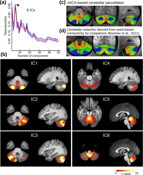
Resting‐state mICA of the cerebellum. (a) The number of components used in the ICA decomposition was derived from the dimensionality‐reproducibility curve (red = mean, blue = 95% confidence intervals), where six was the global maximum. (b) Local functional connectivity networks in the cerebellum detected by mICA. (c) Parcellation of the cerebellum derived from mICA results by assigning each voxel the IC with the highest z‐value. (d) Parcellation derived from connectivity of each voxel with cerebral networks [Buckner et al., 2011]. [Color figure can be viewed in the online issue, which is available at http://wileyonlinelibrary.com.]

Cerebellar mICA components are shown in Figure 2b. Two ICs (IC 2 and IC 3) showed a symmetric lateralized appearance, while all other components were intrinsically symmetric. Comparing our results to a probabilistic cerebellar atlas [Diedrichsen et al., 2009], we found that IC 1 encompassed regions of the left and right cerebellar Crus I‐II. Both IC 2 and IC 3 comprised regions from ipsilateral cerebellar Crus I & II and ipsilateral VI & VIIb. IC 4 included regions of the left and right lobules VI, VIIb, and VIIIa. IC 5 extended over left and right lobules I‐VI as well as vermis lobule VI, while IC 6 comprised left and right cerebellar lobules VIIIb and IX‐X as well as vermis VIIIa and IX‐X.

A parcellation of the cerebellum based on these ICs is shown in Figure 2c. Cerebellar subregions detected by another study [Buckner et al., 2011] are depicted in Figure 2d for comparison. Although a different approach of mapping cerebellar voxels according to their connectivity with seven cerebral networks was used in that study, the results were comparable to our mICA‐based parcellation.

All cerebellar networks showed unique patterns of functional connectivity with other brain regions (Fig. 3). Both IC 1 and IC 6 exhibited similarity with the DMN. IC 2 and IC 3 showed similar (although mirrored) connectivity profiles with close similarity to the frontoparietal control system [Vincent et al., 2008], while IC 2 alone exhibited a strong anti‐correlation with the sensorimotor network. Global connectivity of IC 4 can be best described as a mixture of primary and secondary visual networks with sensorimotor and dorsal attention network, while IC5's connectivity was not similar to any known resting state network.

Figure 3.

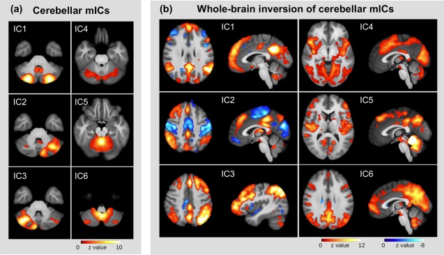
Back‐reconstruction of whole‐brain networks from local cerebellar networks derived by mICA. (a) Cerebellar networks, (b) associated whole‐brain networks, derived by direct back‐reconstruction. [Color figure can be viewed in the online issue, which is available at http://wileyonlinelibrary.com.]

Hippocampus

The hippocampal reproducibility curve of mICA results was different from the cerebellar, in that it showed a high reproducibility (r > 0.85) for a wide range of dimensions with several local maxima (Fig. 4a) and a global maximum at four dimensions. For a number of dimensionalities, mICA did not converge in some of the subsampling groups (Fig. 4b). Based on previous reports [Chase et al., 2015] and our own results [Blessing et al., 2016], we expected at least 3 functionally unique subregions in each hippocampus. Therefore, we chose the first local maximum of the reproducibility curve with 6 or more components that did not show a significant amount of non‐converging mICAs [Chase et al., 2015]. This value was 12 and yielded a reproducibility of r = 0.91 ± 0.047 (mean ± SD). It was selected for the following group‐level and single‐subject mICA analyses. To prove the validity of our recommended approach to use the global maximum of reproducibility curve, we repeated the analysis with a dimensionality of four. The results can be found in Supporting Information Figure 3.

Figure 4.

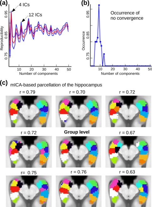
Resting‐state mICA of the hippocampus. (a) The number of components used in the ICA decomposition was derived from the dimensionality‐reproducibility curve (red = mean, blue = 95% confidence intervals), where 12 was a local maximum and lower maxima led non‐convergence of some ICAs (b). The four‐dimensional case (global maximum of the reproducibility curve) can be found in Supporting Information Figure 3. (c) Parcellation of the hippocampus into functionally‐defined subregions derived from mICA results by assigning each voxel the IC with the highest z‐value. The group‐level pattern shows three subregions in the anterior part of the hippocampus: anterior (purple + green), anteromedial (yellow + dark blue), and anterolateral (black + turquoise), one in the mid (red + light blue) and two in the posterior part (white + beige, green + brown). The overall group‐level (n = 50) pattern was reproducible on the single‐subject level as evidenced by eight random subjects with spatial correlation coefficients ranging from 0.63 to 0.79. [Color figure can be viewed in the online issue, which is available at http://wileyonlinelibrary.com.]

Group‐level parcellation of the hippocampus resulted in a roughly symmetrical division of each hippocampus into six longitudinally discrete subregions (anterior, anteromedial, anterolateral, mid and two posterior divisions). For all subjects, except those whose mICA did not converge (3 out of 50), visual inspection revealed similar hippocampal subregions compared to group‐level parcellation. The mean correlation between single‐subject and group‐level parcellations was 0.691 ± 0.059. Figure 4c shows eight randomly chosen single‐subject parcellations compared to the group‐level results. Global connectivity results for the hippocampus can be found in Supporting Information Fig. 3.

Brainstem

The reproducibility curve of brainstem mICA showed three local maxima at 4, 9, and 16 dimensions (Fig. 4d). We chose the value with the highest reproducibility, which was 9. Resulting mICA showed three ICs with significant correlations with the tongue‐movement time‐course. The IC with the highest correlation (z = 16.66) comprised the region of the bilateral hypoglossal nucleus, facial motor nucleus, and spinal trigeminal nucleus (pars oralis) (Fig. 5) while the other two were in the pontine (z = 11.92) and mesencephalic reticular formation (z = 3.13).

Figure 5.

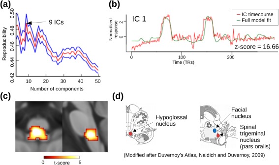
Masked ICA for brainstem‐fMRI analysis of a tongue‐movement task. (a) The number of components used in the ICA decomposition was derived from the dimensionality‐reproducibility curve (red = mean, blue = 95% confidence intervals) with nine being the global maximum. (b) Group‐average time‐course of the IC (red) that showed the highest temporal correlation with the tongue‐movement paradigm (green). (c) Spatial components of that IC. Comparison with a brainstem atlas [Naidich et al., 2008] shows that the activation cluster comprises the bilateral hypoglossal nucleus (the main motor nucleus of tongue movement) as well as the facial and spinal trigeminal nuclei (both of which process sensory information from the inside of the mouth). [Color figure can be viewed in the online issue, which is available at http://wileyonlinelibrary.com.]

The hypoglossal nerve innervates all muscles of the tongue, and the hypoglossal nucleus contains cell bodies of these motoneuron axonal processes. The trigeminal nucleus pars oralis receives sensory input from the oral cavity, a region stimulated by the tongue movement.

Global connectivity results for the brainstem can be found in Supporting Information Fig. 4.

Discussion

In this article, we have introduced the mICA toolbox, a GUI‐based program that facilitates performing mICA and related analyses. We have applied the toolbox to a freely available dataset of state‐of‐the‐art fMRI data, the Human Connectome Dataset. Our results show that the mICA toolbox successfully performs mICA, global connectivity estimation, mICA‐based parcellation, and reproducibility analysis.

Several studies have revealed advantages of exploring fMRI datasets using mICA [Beissner et al., 2014; Dobromyslin et al., 2012; Igelström et al., 2015; Kong et al., 2014; Rebola et al., 2012; Sohn et al., 2012]. One advantage is the ability to detect local connectivity networks, especially for some brain regions (e.g., the brainstem) where other analysis approaches usually fail to reveal prudent results [Beissner et al., 2014]. Global connectivity of masked ICs, conversely, sheds light on the role played by those local networks in the known large‐scale (i.e., whole‐brain) networks. In this regard, the mICA toolbox offers a state‐of‐the‐art approach for studying brain function, by combining these functions in a streamlined, easily accessible manner.

As evident for cerebellar results, local connectivity networks detected by mICA were not merely parts of known whole‐brain networks. Our results from the cerebellum indicate that despite much similarity between them, there are also clear differences evident from visual inspection. Similar findings have also been reported by Dobromyslin et al., [2012]. For example, cerebellar mICA detected two symmetric networks (IC 2 and 3) each comprising lobuli Crus I and II, as well as VI and VIIb. The global connectivity of these respective networks was highly similar to the left and right frontoparietal control system, as previously shown in whole‐brain ICA studies [Vincent et al., 2008].

MICA components provide information about functional heterogeneity inside a studied region, allowing for parcellation into functionally discrete subregions. The hippocampus is a highly suitable brain structure with which to test this functionality of mICA. Both animal models and human functional neuroimaging studies suggest the hippocampus is comprised of discrete subregions along the anterior–posterior axis, which fundamentally differ in function, gene expression, and anatomical connections [Blessing et al., 2016; Strange et al., 2014]. Individual seed based analyses of resting state data in human show that the anterior and posterior hippocampal segments exhibit distinct patterns of functional connectivity [Chase et al., 2015; Kahn et al., 2008]. Resulting ICs in our mICA analysis had a longitudinally discrete configuration, consistent with previous studies. Furthermore, greater heterogeneity (three ICs) was apparent in the anterior hippocampus, as compared to the mid and posterior hippocampus (one an two ICs, respectively); this is consistent with animal models, in which the (equivalent) anterior hippocampus has at least three distinct gene expression and functional domains [Fanselow and Dong, 2010].

Hippocampal ICs produced by mICA were also highly reproducible, providing a means to functionally parcellate the hippocampus in a reproducible manner between data sets. Given the lack of consensus in the definition of hippocampus functional subregions [Poppenk et al., 2013], mICA has great potential for determining the differential global connectivity of functional hippocampus subregions, in a manner that is reproducible between studies. Furthermore, this high reproducibility extended to the single‐subject level, thus enabling calculation of participant‐level functional connectivity of specific hippocampal ICs, which could potentially be correlated with individual measures such as task related activation [Mennes et al., 2010], or clinically relevant variables.

For the brainstem, we were able to replicate our previous results, showing that mICA is capable of detecting BOLD signals from single brainstem nuclei, by excluding noise‐affected regions with a brainstem mask [Beissner et al., 2014]. While our original study used rfMRI data, we show in this article that the approach works equally well with task‐based data. MICA successfully detected the bilateral hypoglossal nucleus together with nuclei of sensory nerves that are stimulated by tongue movement. Since a brainstem mask is included in the Harvard‐Oxford atlas that comes with FSL, the mICA toolbox should also facilitate otherwise complex brainstem‐fMRI analyses [Beissner, 2015]. However, for reasons unknown we did not observe significant whole‐brain connectivity for our main brainstem component. We can only speculate that this may have been due to the relatively low decomposition dimensionality of d = 9 that might have led to an incomplete splitting of sensory and motor regions in the brainstem. Another possible explanation is that the imaging protocol of the HCP data was not optimized for the brainstem region.

Some limitations of the toolbox need to be discussed. First, the current reproducibility‐based approach for the selection of an optimal mICA dimensionality is rather simplistic: It identifies matching ICs between two samplings by means of cross‐correlation analysis, and then uses the average correlation value as a measure of reproducibility. Future releases should preferably use more sophisticated methods for matching of components as well as for reproducibility analysis [Esposito et al., 2005; Pendse et al., 2011; Wang and Peterson, 2008]. For example, with our approach we cannot be entirely sure that the reproducible ICs from a pair of split‐half samples are similar to those from another pair of samples. Furthermore, using the mean correlation of all matched IC‐pairs as a reproducibility measure might be suboptimal, in particular when comparing reproducibility of ICAs with different dimensionalities. For example, increasing dimensionality may lead to greater stability of “true” components but at the same time cause over‐splitting of noise‐related components. While this would seemingly reduce reproducibility, a higher dimensionality might still be a favorable choice. It would thus be desirable to have an automated method to differentiate true components from noise and then only track the former. For whole‐brain analyses, some approaches using machine learning classifiers have recently been introduced [Griffanti et al., 2014; Salimi‐Khorshidi et al., 2014] and may be adapted for this problem.

We have recommended some guidelines for how to select the best dimensionality from the reproducibility curve. In our opinion, the global maximum is a good first approach and should be used whenever possible. A reproducibility‐based approach to choose ICA dimensionality may be a viable alternative to information‐theoretic approaches, since reproducibility of results is one of the most important objectives of the scientific method. There may, however, be cases where a priori information (as used for the hippocampus, see Figure 4) should also be taken into account.

Second, our parcellation approach based on the mICA results assigns each voxel to the IC with the highest z‐score. This approach could also be improved using more sophisticated methods, like advanced clustering algorithms, to reflect the uncertainty in areas where multiple components overlap, or where z‐scores are low.

Future work should investigate in more detail how mICA performs in comparison to whole‐brain ICA. While it is evident from our preliminary results that there are differences between masked ICs and the same regions of whole‐brain ICs, these have been derived using the same dimensionality for both analyses. It may thus be that high‐dimensional whole‐brain ICA may produce results that are more similar to low‐dimensional mICA. Furthermore, it remains to be shown how masking affects the detection of physiological noise in fMRI data. Whole‐brain ICA is usually successful in disentangling mixed sources of signal and noise across the brain. However, if noise‐affected regions, like the ventricles are masked out, noise signals may get absorbed into the detected components and either become a component by itself or negatively affect other components.

To conclude, we have shown that mICA is a useful tool for fc analyses of small brain regions. It can extract information on local connectivity networks, and can aid with the functional segmentation of structures, like the hippocampus. Furthermore, it offers the only current approach, to our knowledge, to study fc in the brainstem by means of ICA. We hope that our toolbox will promote the mICA approach, and facilitate understanding of how local connectivity networks interrelate with those on the global scale.

Supporting information

Supporting Information

Supporting Information

Supporting Information

Supporting Information

Supporting Information

REFERENCES

- Baria AT, Mansour A, Huang L, Baliki MN, Cecchi GA, Mesulam MM, Apkarian AV (2013): Linking human brain local activity fluctuations to structural and functional network architectures. Neuroimage 73:144–155. [DOI] [PMC free article] [PubMed] [Google Scholar]
- Beckmann CF, Smith SM (2005): Tensorial extensions of independent component analysis for multisubject FMRI analysis. Neuroimage 25:294–311. [DOI] [PubMed] [Google Scholar]
- Beckmann CF, DeLuca M, Devlin JT, Smith SM (2005): Investigations into resting‐state connectivity using independent component analysis. Philos Trans R Soc Lond B Biol Sci 360:1001–1013. [DOI] [PMC free article] [PubMed] [Google Scholar]
- Beckmann CF, Smith SM (2004): Probabilistic Independent Component Analysis for Functional Magnetic Resonance Imaging. IEEE Trans Med Imaging 23:137–152. [DOI] [PubMed] [Google Scholar]
- Beckmann M, Filippini S (2009): Group comparison of resting‐state FMRI data using multi‐subject ICA and dual regression. Neuroimage 47:S148. [Google Scholar]
- Beissner F (2015): Functional MRI of the brainstem: Common problems and their solutions. Clin Neuroradiol 25:251–257. [DOI] [PubMed] [Google Scholar]
- Beissner F, Deichmann R, Baudrexel S (2011): FMRI of the brainstem using dual‐echo EPI. Neuroimage 55:1593–1599. [DOI] [PubMed] [Google Scholar]
- Beissner F, Schumann A, Brunn F, Eisenträger D, Bär KJ (2014): Advances in functional magnetic resonance imaging of the human brainstem. Neuroimage 86:91–98. [DOI] [PubMed] [Google Scholar]
- Blessing EM, Beissner F, Schumann A, Brünner F, Bär KJ (2016): A data‐driven approach to mapping cortical and subcortical intrinsic functional connectivity along the longitudinal hippocampal axis. Hum Brain Mapp 37:462–476. [DOI] [PMC free article] [PubMed] [Google Scholar]
- Buckner RL, Krienen FM, Castellanos A, Diaz JC, Yeo BTT (2011): The organization of the human cerebellum estimated by intrinsic functional connectivity. J Neurophysiol 106:2322–2345. [DOI] [PMC free article] [PubMed] [Google Scholar]
- Bzdok D, Laird AR, Zilles K, Fox PT, Eickhoff SB (2013): An investigation of the structural, connectional, and functional subspecialization in the human amygdala. Hum Brain Mapp 34:3247–3266. [DOI] [PMC free article] [PubMed] [Google Scholar]
- Calhoun VD, Adali T, Pearlson GD, Pekar JJ (2001): A method for making group inferences from functional MRI data using independent component analysis. Hum Brain Mapp 14:140–151. [DOI] [PMC free article] [PubMed] [Google Scholar]
- Chase HW, Clos M, Dibble S, Fox P, Grace AA, Phillips ML, Eickhoff SB (2015): Evidence for an anterior–posterior differentiation in the human hippocampal formation revealed by meta‐analytic parcellation of fMRI coordinate maps: Focus on the subiculum. Neuroimage 113:44–60. [DOI] [PMC free article] [PubMed] [Google Scholar]
- Collins D, Holmes C, Peters T, Evans a (1995): Automatic 3‐D model‐based neuroanatomical segmentation. Hum Brain Mapp 208:190–208. [Google Scholar]
- Damoiseaux JS, Greicius MD (2009): Greater than the sum of its parts: A review of studies combining structural connectivity and resting‐state functional connectivity. Brain Struct Funct 213:525–533. [DOI] [PubMed] [Google Scholar]
- Diedrichsen J, Balsters JH, Flavell J, Cussans E, Ramnani N (2009): A probabilistic MR atlas of the human cerebellum. Neuroimage 46:39–46. [DOI] [PubMed] [Google Scholar]
- Dobromyslin VI, Salat DH, Fortier CB, Leritz EC, Beckmann CF, Milberg WP, McGlinchey RE (2012): Distinct functional networks within the cerebellum and their relation to cortical systems assessed with independent component analysis. Neuroimage 60:2073–2085. [DOI] [PMC free article] [PubMed] [Google Scholar]
- Esposito F, Scarabino T, Hyvarinen A, Himberg J, Formisano E, Comani S, Tedeschi G, Goebel R, Seifritz E, Di Salle F (2005): Independent component analysis of fMRI group studies by self‐organizing clustering. Neuroimage 25:193–205. [DOI] [PubMed] [Google Scholar]
- Van Essen DC, Smith SM, Barch DM, Behrens TEJ, Yacoub E, Ugurbil K (2013): The WU‐Minn Human Connectome Project: An overview. Neuroimage 80:62–79. [DOI] [PMC free article] [PubMed] [Google Scholar]
- Vincent JL, Kahn I, Snyder AZ, Raichle ME, Buckner RL (2008): Evidence for a frontoparietal control system revealed by intrinsic functional connectivity. J Neurophysiol 100:3328–3342. [DOI] [PMC free article] [PubMed] [Google Scholar]
- Fanselow MS, Dong H‐W (2010): Are the dorsal and ventral hippocampus functionally distinct structures? Neuron 65:7–19. [DOI] [PMC free article] [PubMed] [Google Scholar]
- Filippini N, MacIntosh BJ, Hough MG, Goodwin GM, Frisoni GB, Smith SM, Matthews PM, Beckmann CF, Mackay CE (2009): Distinct patterns of brain activity in young carriers of the APOE‐epsilon4 allele. Proc Natl Acad Sci USA 106:7209–7214. [DOI] [PMC free article] [PubMed] [Google Scholar]
- Frazier JA, Chiu S, Breeze JL, Makris N, Lange N, Kennedy DN, Herbert MR, Bent EK, Koneru VK, Dieterich ME, Hodge SM, Rauch SL, Grant PE, Cohen BM, Seidman LJ, Caviness VS, Biederman J (2005): Structural brain magnetic resonance imaging of limbic and thalamic volumes in pediatric bipolar disorder. Am J Psychiatry 162:1256–1265. [DOI] [PubMed] [Google Scholar]
- Glasser MF, Sotiropoulos SN, Wilson JA, Coalson TS, Fischl B, Andersson JL, Xu J, Jbabdi S, Webster M, Polimeni JR, Van Essen DC, Jenkinson M (2013): The minimal preprocessing pipelines for the Human Connectome Project. Neuroimage 80:105–124. [DOI] [PMC free article] [PubMed] [Google Scholar]
- Griffanti L, Salimi‐Khorshidi G, Beckmann CF, Auerbach EJ, Douaud G, Sexton CE, Zsoldos E, Ebmeier KP, Filippini N, Mackay CE, Moeller S, Xu J, Yacoub E, Baselli G, Ugurbil K, Miller KL, Smith SM (2014): ICA‐based artefact removal and accelerated fMRI acquisition for improved resting state network imaging. Neuroimage 95:232–247. [DOI] [PMC free article] [PubMed] [Google Scholar]
- Igelström K, Webb T, Graziano M (2015): Neural processes in the human temporoparietal cortex separated by localized independent component analysis. J Neurosci 35:9432–9445. [DOI] [PMC free article] [PubMed] [Google Scholar]
- Jenkinson M, Beckmann CF, Behrens TEJ, Woolrich MW, Smith SM (2012): FSL. Neuroimage 62:782–790. [DOI] [PubMed] [Google Scholar]
- Kahn I, Andrews‐Hanna JR, Vincent JL, Snyder AZ, Buckner RL (2008): Distinct cortical anatomy linked to subregions of the medial temporal lobe revealed by intrinsic functional connectivity. J Neurophysiol 100:129–139. [DOI] [PMC free article] [PubMed] [Google Scholar]
- Kim JH, Lee JM, Jo HJ, Kim SH, Lee JH, Kim ST, Seo SW, Cox RW, Na DL, Kim SI, Saad ZS (2010): Defining functional SMA and pre‐SMA subregions in human MFC using resting state fMRI: Functional connectivity‐based parcellation method. Neuroimage 49:2375–2386. [DOI] [PMC free article] [PubMed] [Google Scholar]
- Kong Y, Eippert F, Beckmann CF, Andersson J, Finsterbusch J, Büchel C, Tracey I, Brooks JCW (2014): Intrinsically organized resting state networks in the human spinal cord. Proc Natl Acad Sci USA 111:18067–18072. [DOI] [PMC free article] [PubMed] [Google Scholar]
- Kuhn HW (1955): The Hungarian method for the assignment problem. Nav Res Logist Q 2:83–97. [Google Scholar]
- Leech R, Braga R, Sharp DJ (2012): Echoes of the brain within the posterior cingulate cortex. J Neurosci 32:215–222. [DOI] [PMC free article] [PubMed] [Google Scholar]
- Li Y‐O, Adali T, Calhoun VD (2007): Estimating the number of independent components for functional magnetic resonance imaging data. Hum Brain Mapp 28:1251–1266. [DOI] [PMC free article] [PubMed] [Google Scholar]
- Mazziotta J, Toga A, Evans A, Fox P, Lancaster J, Zilles K, Woods R, Paus T, Simpson G, Pike B, Holmes C, Collins L, Thompson P, MacDonald D, Iacoboni M, Schormann T, Amunts K, Palomero‐Gallagher N, Geyer S, Parsons L, Narr K, Kabani N, Le Goualher G, Boomsma D, Cannon T, Kawashima R, Mazoyer B (2001): A probabilistic atlas and reference system for the human brain: International Consortium for Brain Mapping (ICBM). Philos Trans R Soc Lond B Biol Sci 356:1293–1322. [DOI] [PMC free article] [PubMed] [Google Scholar]
- McKeown MJ, Makeig S, Brown GG, Jung TP, Kindermann SS, Bell AJ, Sejnowski TJ (1998): Analysis of fMRI data by blind separation into independent spatial components. Hum Brain Mapp 6:160–188. [DOI] [PMC free article] [PubMed] [Google Scholar]
- Mennes M, Kelly C, Zuo XN, Di Martino A, Biswal BB, Castellanos FX, Milham MP (2010): Inter‐individual differences in resting‐state functional connectivity predict task‐induced BOLD activity. Neuroimage 50:1690–1701. [DOI] [PMC free article] [PubMed] [Google Scholar]
- Munkres J (1957): Algorithms for the Assignment and Transportation Problems. J Soc Ind Appl Math 5:32–38. [Google Scholar]
- Naidich TP, Duvernoy HM, Delman BN, Sorensen AG, Kollias SS, Haacke EM (2008): Duvernoy's Atlas of the Human Brain Stem and Cerebellum: High‐Field MRI, Surface Anatomy, Internal Structure, Vascularization and 3 D Sectional Anatomy. Wien, New York: Springer. [Google Scholar]
- Pendse GV, Borsook D, Becerra L (2011): A simple and objective method for reproducible resting state network (RSN) detection in fMRI. Ed. Wang Zhan. PLoS One 6:e27594. [DOI] [PMC free article] [PubMed] [Google Scholar]
- Poppenk J, Evensmoen HR, Moscovitch M, Nadel L (2013): Long‐axis specialization of the human hippocampus. Trends Cogn Sci 17:230–240. [DOI] [PubMed] [Google Scholar]
- Raichle ME, MacLeod AM, Snyder AZ, Powers WJ, Gusnard DA, Shulman GL (2001): A default mode of brain function. Proc Natl Acad Sci USA 98:676–682. [DOI] [PMC free article] [PubMed] [Google Scholar]
- Ray KL, McKay DR, Fox PM, Riedel MC, Uecker AM, Beckmann CF, Smith SM, Fox PT, Laird AR (2013): ICA model order selection of task co‐activation networks. Front Neurosci 7:237. [DOI] [PMC free article] [PubMed] [Google Scholar]
- Rebola J, Castelhano J, Ferreira C, Castelo‐Branco M (2012): Functional parcellation of the operculo‐insular cortex in perceptual decision making: An fMRI study. Neuropsychologia 50:3693–3701. [DOI] [PubMed] [Google Scholar]
- Salimi‐Khorshidi G, Douaud G, Beckmann CF, Glasser MF, Griffanti L, Smith SM (2014): Automatic denoising of functional MRI data: Combining independent component analysis and hierarchical fusion of classifiers. Neuroimage 90:449–468. [DOI] [PMC free article] [PubMed] [Google Scholar]
- Shen X, Papademetris X, Constable RT (2010): Graph‐theory based parcellation of functional subunits in the brain from resting‐state fMRI data. Neuroimage 50:1027–1035. [DOI] [PMC free article] [PubMed] [Google Scholar]
- Smith SM, Smith SM, Jenkinson M, Jenkinson M, Woolrich MW, Woolrich MW, Beckmann CF, Beckmann CF, Behrens TEJ, Behrens TEJ, Johansen‐Berg H, Johansen‐Berg H, Bannister PR, Bannister PR, De Luca M, De Luca M, Drobnjak I, Drobnjak I, Flitney DE, Flitney DE, Niazy RK, Niazy RK, Saunders J, Saunders J, Vickers J, Vickers J, Zhang Y, Zhang Y, De Stefano N, De Stefano N, Brady JM, Brady JM, Matthews PM, Matthews PM (2004): Advances in functional and structural MR image analysis and implementation as FSL. Neuroimage 23:S208–S219. [DOI] [PubMed] [Google Scholar]
- Smith SM, Beckmann CF, Andersson J, Auerbach EJ, Bijsterbosch J, Douaud G, Duff E, Feinberg DA, Griffanti L, Harms MP, Kelly M, Laumann T, Miller KL, Moeller S, Petersen S, Power J, Salimi‐Khorshidi G, Snyder AZ, Vu AT, Woolrich MW, Xu J, Yacoub E, Uǧurbil K, Van Essen DC, Glasser MF (2013): Resting‐state fMRI in the Human Connectome Project. Neuroimage 80:144–168. [DOI] [PMC free article] [PubMed] [Google Scholar]
- Smith SM, Nichols TE (2009): Threshold‐free cluster enhancement: Addressing problems of smoothing, threshold dependence and localisation in cluster inference. Neuroimage 44:83–98. [DOI] [PubMed] [Google Scholar]
- Sohn WS, Yoo K, Jeong Y (2012): Independent component analysis of localized resting‐state functional magnetic resonance imaging reveals specific motor subnetworks. Brain Connect 2:218–224. [DOI] [PubMed] [Google Scholar]
- Strange BA, Witter M, Lein E, Moser E (2014): Functional organization of the hippocampal longitudinal axis. Nat Rev Neurosci 15:655–669. [DOI] [PubMed] [Google Scholar]
- Wang Z, Peterson BS (2008): Partner‐matching for the automated identification of reproducible ICA components from fMRI datasets: Algorithm and validation. Hum Brain Mapp 29:875–893. [DOI] [PMC free article] [PubMed] [Google Scholar]
- Winkler AM, Ridgway GR, Webster MA, Smith SM, Nichols TE (2014): Permutation inference for the general linear model. Neuroimage 92:381–397. [DOI] [PMC free article] [PubMed] [Google Scholar]
- Woolrich MW, Behrens TEJ, Beckmann CF, Smith SM (2005): Mixture models with adaptive spatial regularization for segmentation with an application to FMRI data. IEEE Trans Med Imaging 24:1–11. [DOI] [PubMed] [Google Scholar]
- Woolrich MW, Jbabdi S, Patenaude B, Chappell M, Makni S, Behrens T, Beckmann C, Jenkinson M, Smith SM (2009): Bayesian analysis of neuroimaging data in FSL. Neuroimage 45:S173–S186. [DOI] [PubMed] [Google Scholar]
- Zuo XN, Kelly C, Adelstein JS, Klein DF, Castellanos FX, Milham MP (2010): Reliable intrinsic connectivity networks: Test‐retest evaluation using ICA and dual regression approach. Neuroimage 49:2163–2177. [DOI] [PMC free article] [PubMed] [Google Scholar]
Associated Data
This section collects any data citations, data availability statements, or supplementary materials included in this article.
Supplementary Materials