Dynamic functional connectivity shapes individual differences in associative learning

Abstract

Current neuroscientific research has shown that the brain reconfigures its functional interactions at multiple timescales. Here, we sought to link transient changes in functional brain networks to individual differences in behavioral and cognitive performance by using an active learning paradigm. Participants learned associations between pairs of unrelated visual stimuli by using feedback. Interindividual behavioral variability was quantified with a learning rate measure. By using a multivariate statistical framework (partial least squares), we identified patterns of network organization across multiple temporal scales (within a trial, millisecond; across a learning session, minute) and linked these to the rate of change in behavioral performance (fast and slow). Results indicated that posterior network connectivity was present early in the trial for fast, and later in the trial for slow performers. In contrast, connectivity in an associative memory network (frontal, striatal, and medial temporal regions) occurred later in the trial for fast, and earlier for slow performers. Time‐dependent changes in the posterior network were correlated with visual/spatial scores obtained from independent neuropsychological assessments, with fast learners performing better on visual/spatial subtests. No relationship was found between functional connectivity dynamics in the memory network and visual/spatial test scores indicative of cognitive skill. By using a comprehensive set of measures (behavioral, cognitive, and neurophysiological), we report that individual variations in learning‐related performance change are supported by differences in cognitive ability and time‐sensitive connectivity in functional neural networks. Hum Brain Mapp 37:3911–3928, 2016. © 2016 Wiley Periodicals, Inc.

INTRODUCTION

Human learning and memory are complex and highly adaptive cognitive processes. When given new tasks to learn, individuals tend to employ unique behavioral and neural strategies [Iaria et al., 2003; Poldrack et al., 2001; Sanfratello et al., 2014] that often reflect inherent predispositions [Luck and Vogel, 2013] and cumulative experiences. Accurate differentiation of neural mechanisms that give rise to behavioral and cognitive flexibility must take into account individual differences [Bassett et al., 2015; Braver et al., 2010]. This line of inquiry is valuable for developing personalized therapies to remediate cognitive impairments across the lifespan (from development to aging); and for creating educational materials that enhance performance for different learning styles. In this study, our main goal was to obtain comprehensive features (behavioral, cognitive, and neurophysiological) that highlighted individual differences in learning novel associations using data‐driven methods.

Conditional associative learning paradigms [Law et al., 2005; Mattfeld and Stark, 2011; Petrides, 1985; Toni and Passingham, 1999], in which participants actively decipher correct relationships between stimuli and responses, are well‐suited for examining individual variability. During the learning process, individuals transition from an early exploratory phase where responses are mainly driven by trial‐and‐error to a later automated phase where responses are retrieved from memory. Transitions from trial‐and‐error to asymptotic performance occur at variable rates across individuals but the trajectory of learning can be quantified for interindividual comparison [Buchel et al., 1999]. In conjunction, neuropsychological test batteries can offer more standardized indices of comparing cognitive skills across individuals. Here, our first aim was to generate composite profiles of learners using their online performance (e.g., accuracy, speed of learning) and intrinsic cognitive ability (e.g., scores on several subtests); and subsequently link these profiles to time‐sensitive functional network organization in the brain.

Previous neuroscientific research posits that adaptive cognitive control depends on coordination of information across local and distributed brain sites [Bressler and Tognoli, 2006; McIntosh, 2000]. This integrative property of the human brain, as expressed in large‐scale functional network interactions (functional connectivity), can be explored in multiple dimensions (e.g., spatiotemporal, spectral, topological, etc.) during active learning [Bassett et al., 2011, 2015; Brovelli et al., 2015]. Our main focus was to establish the link between whole‐brain functional connectivity derived from two different temporal scales (across the learning session, minutes; within trials of learning, milliseconds) with individual differences in performance measures (rate of learning) and cognitive ability (neuropsychological test scores). While support for time‐varying analyses of connectivity are growing in the literature [Allen et al., 2014; Di and Biswal, 2015; Fu et al., 2013; Handwerker et al., 2012; Hutchison et al., 2013], the applicability of these methods for understanding brain–behavior relationships still remains to be determined.

We made several methodological choices in this study to enable us to assess relationships across multiple indices of associative learning (speed, accuracy, cognitive skill, functional network organization at two time scales). First, we acquired neurophysiological data with magnetoencephalography (MEG), a neuroimaging modality with good spatial and temporal resolution. We also adopted an analysis method that was sensitive to transient changes in whole‐brain network dynamics [Allen et al., 2014]. Rather than calculate functional connectivity between source pairs over the entire time series [Friston, 1995], connectivity was computed in short time windows spanning the duration of a learning trial (see review of method: Hutchison et al. [2013]). Patterns embedded in multidimensional data were extracted and validated using partial least squares (PLS) [McIntosh and Lobaugh 2004]. PLS is optimized to identify relationships within multidimensional MEG data [Cheung et al., 2016] and has successfully been used in a wide range of MEG studies on cognition [Duzel et al., 2003; Fatima et al., 2013; Hopf et al., 2013; McIntosh et al., 2013; Misic et al., 2010, 2014]. By employing a combination of methods (novel and typical), we sought to identify holistic (behavioral, cognitive, and neurophysiological) markers of individual differences in acquiring novel associations.

MATERIALS AND METHODS

Participants

Fourteen right‐handed young adults (8 female) between the ages of 19 and 30 (mean age: 22 ± 2 years) participated in the study. All participants had normal to corrected vision. Exclusion criteria included any metal implants, neurological, psychiatric, and substance abuse‐related problems. Participants gave consent in accordance with the joint Baycrest Centre‐University of Toronto Research Ethics Committee.

Stimuli and Apparatus

Two types of visual stimuli were used: scenes and colors. Four scene pairs were chosen from a photograph repository [Riggs et al., 2009] based on the similarity of their composition (content, lines, edges, landmark features, etc.). There were 2 fireplace scenes (indoor), 2 kitchen scenes (indoor), 2 mountain views (outdoor), and 2 seascapes (outdoor). All scenes were converted to grayscale with equal mean luminance so that a color‐based strategy for encoding scene content was discouraged and instead, participants had to focus on binding the spatial elements of the scene (important for associative learning, see later discussion). The second set of stimuli consisted of circles in 8 distinct colors: red, blue, yellow, green, magenta, cyan, orange, and pink.

All visual stimuli were displayed with an NEC projector (model NP215) on a translucent screen that hung above the MEG scanner. Distance of the screen from the participant was approximately 1.68 m with horizontal and vertical angles of 50.5° and 39.5°, respectively. Scenes filled the entire screen display at a resolution of 1024 × 768 pixels while colors were shown on a black background, placed on the left and right side of a fixation cross in the center of the screen (see Fig. 1 for schematic). A white square (38 × 38 pixels) was projected on the top right‐hand corner of each screen with a visual stimulus, outside the participant's field of view. Luminance changes, detected by a photodiode, signaled the presence or absence of a visual stimulus (white square when stimulus was on, no square (black space) when stimulus was off). Photodiode pulses recorded by the acquisition computer were later used to obtain precise timing information about stimulus events in line with best practices [Gross et al., 2013]. Participants responded to the colored circles with left or right button press (index finger). Fiber‐optic response paddles recorded responses. These devices were constructed at the Rotman Research Institute with custom nonmagnetic parts. Stimulus delivery and response data collection were enabled by Presentation software (version 14.5, Neurobehavioural Systems Inc.).

Figure 1.

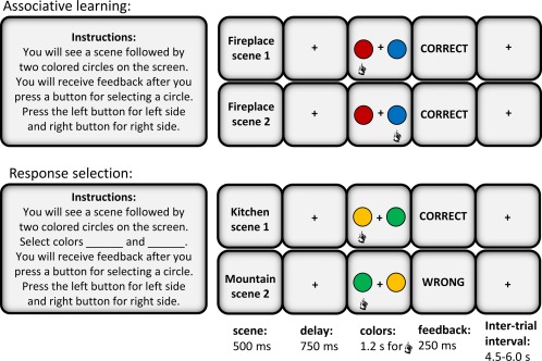
Task parameters. Details related to experimental design are shown here for the associative learning and response selection task. In associative learning, participants have to learn the correct deterministic relationship between a particular scene and a particular color. The same color pair (e.g., red, blue) is always associated with the same scene pair (e.g., fireplace 1, 2). Each scene is presented separately (with equal probability of 0.25, each scene presented 38 times) but the colors appear in pairs. Participants receive onscreen feedback (correct/wrong) after response execution. Associations between color pairs and scene pairs are assigned randomly for each participant and unique stimuli are used for each task. In the response selection task, participants are told which color to select in the instructions. Scenes in the response selection task bear no relationship to upcoming color pairs. For simplicity, 2 out of 4 stimulus pairs are displayed and the scenes are replaced with text. The hand symbol indicates the response chosen for this example. [Color figure can be viewed at http://wileyonlinelibrary.com.]

Task Design Parameters

MEG data recordings consisted of two task blocks—associative learning (experimental task) and response selection (control task)—with 152 trials of each type (Fig. 1). In the associative learning task, participants had to learn the conditional relationship between scene–color pairs (e.g., fireplace 1‐red circle, fireplace 2‐blue circle). The conditional associative relationships in the task were deterministic: same color pair (e.g., red, blue) was always associated with the same scene pair (e.g., fireplace 1, 2). Participants had to learn a total of 4 scene–color associations (with equal probability of 0.25, each scene presented 38 times) using trial‐and‐error. Scenes were presented one at a time for 500 ms followed by a delay of 750 ms. Then, the color pair would be displayed for up to 1.2 s during which time participants had to select a color (left/right button press to indicate left/right color choice). A particular color was equally likely to appear in the left or the right spatial location (separated by fixation cross) and the location had no relevance for learning. After responses were made, participants received on‐screen written feedback (correct, wrong). The trial ended with a randomized intertrial interval between 4.5 and 6 s. The response selection task was designed as a control task with no learning component. Participants were informed of which colors would yield “correct” feedback. Trial structure for the control task was identical to the learning task except scenes were presented randomly and were not related to upcoming color pairs.

Each task (associative learning, response selection) had a unique set of stimuli, taken at random from the stimulus pool (4 scene pairs, 4 colors). Scene–color assignments were fully randomized across participants, scene presentations were randomized within experimental sessions, and the order in which tasks were performed was also counterbalanced (e.g., associative learning first, response selection second; or vice versa).

MEG Data Acquisition

MEG recordings were acquired at Baycrest Centre in a magnetically shielded room with a 151‐channel whole‐head axial gradiometer system (VSM‐Med Tech Inc., Coquitlam, BC, Canada) that had receiver coils uniformly spaced approximately 3 cm apart on a helmet‐shaped array. Participants lay in supine position during data acquisition to minimize motion artifacts. Two MEG recording sessions, 18 min each, took place (one for each task). The data sampling rate was 625 Hz. Head position was documented at the beginning and the end of every data session with 3 indicator coils (nasion, left/right preauricular). Motion tolerance was set to 0.5 cm and all participants fell within this limit.

In addition to MEG, a structural magnetic resonance image (MRI) was also acquired for coregistration purposes. This image was a 3D MPRAGE T1‐weighted pulse sequence (echo time, 2.6 ms; repetition time, 2 s; 256 × 256 acquisition matrix; voxel size,1.0 × 1.0 × 1.0 mm) from a 3T magnet (Siemens Magnetrom TIM Trio Whole Body scanner) located at Baycrest Centre.

Debriefing Questionnaire and Neuropsychological Test Battery

Following data acquisition, participants filled out a debriefing pamphlet that had questions related to task difficulty, type of strategy used to learn novel associations, and an explicit statement describing the exact scene–color relationships set by the experimenters. Participants did not find the tasks difficult: mean ratings were 1.93 ± 0.70 on a five‐point scale (1 for easy, 5 for very difficult). Participants also explicitly named the scenes presented to them and informed us of the exact relationship between scene–color pairs.

To link behavioral performance during learning to independent measures of cognitive ability, a series of standardized neuropsychological tests were administered. Order effects were minimized by counterbalancing the test sequence across participants. The battery included tests for memory (Designs and Logical Memory subtests were taken from the Wechsler Memory Scale – IV [Wechsler, 2009]) and executive function (Phonemic Fluency ‐ word generation by letters F, A, S in 1 min [Spreng et al., 2013], and Digit Span (Forward, Backward, Sequence) from the Wechsler Adult Intelligence Scale [Wechsler, 2008]). Mean scores in each subtest are shown in Supporting Information, Table S1.

Neuropsychological data was first analyzed using pairwise correlations to determine the structure of dependencies among test scores. Results from this preliminary analysis suggested grouping of test scores into three clusters (Supporting Information, Fig. S1). A more detailed clustering analysis on the data was performed with principal component analysis (PCA).

Dimensionality Reduction of Neuropsychological Data

PCA helped identify which test categories shared common cognitive features and simultaneously reduced dimensionality of data into fewer variables that could be correlated with behavioral indices from the study (learning rate, in particular). The output from PCA was a set of orthogonal principal components (PCs: linear combination of original variables) that were ranked in order of the variance they accounted for in the original data [Abdi and Williams, 2010]. Not all computed PCs were retained for further analysis and here, the decision was made to retain PCs based on the consensus reached between the Scree plot and Kaiser's rule [Jolliffe, 2002].

Learning Curve Approximation

Every learning trial was scored as correct (1) or incorrect (0). To capture behavioral changes that spanned the entire learning session, accuracy (proportion of correct responses) was plotted on a continuum with temporal smoothing. Moving average windows consisting of different trial lengths (4, 6, 8, 10, and 12) were systematically evaluated across individuals. The goal was to obtain a smoothing factor (number of trials) that provided the best single parameter fit of the exponential function for all individuals. The function taken from Buchel et al. [1999] for estimating learning rate was

$$f\left(x\right)=1-{\mathrm{e}}^{-\mathit{k}\mathrm{x}}, 0<\mathit{k}<1$$

The k parameter was bound between 0 and 1 with values near 0 indicating slower rates. On the graph, higher values of k translated into a function with steeper curvature (see Fig. 3 for example). The Curve Fitting toolbox (The MathWorks, http://www.mathworks.com/products/curvefitting/) was used for estimating participant‐specific curves. The fitting method for a custom exponential equation was set to nonlinear least squares, with robust least squares regression (LAR), to reduce the impact of extreme values.

Figure 3.

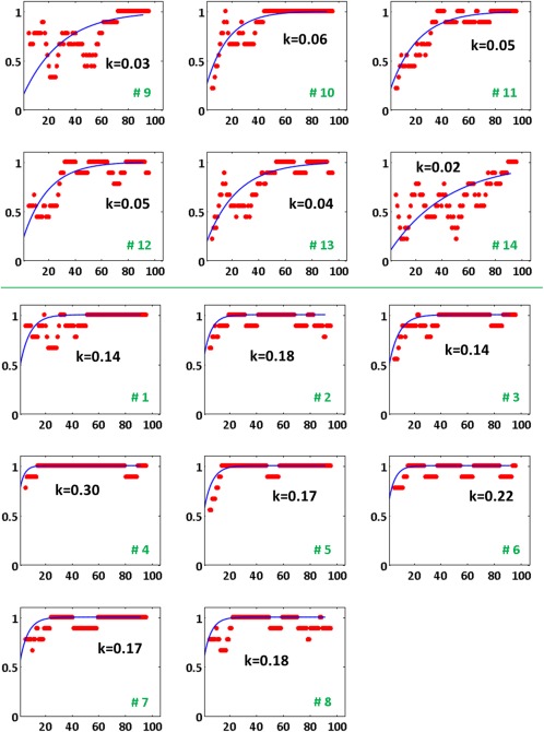
Learning curves for all participants. Top panel: learners with slow rate estimates (lower k). Bottom panel: learners with fast rate estimates (higher k). Learners were divided into fast and slow groups using a mean split (k = 0.12). Participant number (in green) for each curve plot is assigned based on the order list from Table 1. Smoothed accuracy values (y‐axis) for trials (x‐axis) are shown as red dots with the blue curve representing the exponential function fit to the data. [Color figure can be viewed at http://wileyonlinelibrary.com.]

The default algorithm (trust‐region) for bound coefficients was used for fitting. The procedure for each nonlinear fit was as follows: a starting value was given for a coefficient and a fitted curve was produced. Next, the coefficient was adjusted to determine whether the fit improved (default settings, ε = 0.1). This iterative process continued until the fit converged or the maximum number of model evaluations/fit iterations was reached. For the present dataset, the fit converged before 600 function evaluations/400 iterations (default settings).

Other indices of goodness of fit that were estimated by the toolbox included r‐square, standard error (root mean square error, RMSE) and 95% confidence intervals. These three indices are listed in Table 1 in addition to the free parameter.

Table 1.

Goodness of fit values for learning rate estimation

Group	k	R‐square	RMSE	Lower CI	Upper CI
Fast Learners
1	0.1367	0.9848	0.0128	0.1340	0.1395
2	0.1831	0.9904	0.0078	0.1803	0.1859
3	0.1373	0.9952	0.0071	0.1358	0.1389
4	0.3008	0.9928	0.0041	0.2970	0.3047
5	0.1690	0.9977	0.0046	0.1676	0.1704
6	0.2149	0.9906	0.0069	0.2116	0.2181
7	0.1671	0.9920	0.0074	0.1649	0.1694
8	0.1880	−0.1840	0.1052	0.1489	0.2271
a	0.1830	0.9888	0.0142	0.1782	0.1883
Slow Learners
9	0.0343	0.9860	0.0236	0.0337	0.0349
10	0.0610	0.9968	0.0106	0.0604	0.0617
11	0.0485	0.8719	0.0770	0.0452	0.0518
12	0.0534	0.6368	0.1178	0.0476	0.0593
13	0.0431	0.6186	0.1277	0.0385	0.0477
14	0.0225	0.1725	0.1886	0.0197	0.0254

Abbreviations: k, learning rate; RMSE, root mean square error; CI, confidence intervals.

^aCurve fits for participant # 8 were performed twice with different smoothing parameters (see “Results” for further details). Participant numbers match those in Figure 3.

Correlation of Behavioral Measures

A correlation analysis was performed to relate individual cognitive ability to observed behavioral performance during the MEG session. Component scores were calculated by projecting the variables onto the PCs [Abdi and Williams, 2010; McIntosh and Misic, 2013] and served as proxies for individual cognitive capacity. The rate parameter from the curve fitting procedure provided a metric for associative learning ability. Score–rate correlations were statistically evaluated with resampling metrics: permutations and bootstraps.

Ten thousand permutation tests were used to assess whether a set of correlations were significantly different from chance [Good, 2000]. For every permutation, the correspondence between PC scores and the rate parameter were randomized without replacement. Next, the score–rate correlations were calculated to generate a null distribution of the correlations. A probability value was assigned based on the number of times the permuted coefficient exceeded the original coefficient. If the permuted P value was less than a critical alpha of 0.05, the score–rate relationship was deemed significantly different from zero.

Bootstrap estimation provided an index of the robustness of the score–rate correlation across participants [Efron and Tibshirani, 1986]. For each of the 5000 bootstraps, the correspondence between PC scores and learning rate were randomized with replacement. The bootstrap distribution was used to derive confidence intervals (90%) for the mean score–rate correlation.

An additional correlation analysis verified whether the subjective experience of participating in the learning task (difficulty ratings from debriefing questionnaire) was related to the rate of acquiring new associations. No statistically significant relationship (r = 0.14, P = 0.63) was found between the rate parameter and task difficulty ratings.

Data Preprocessing and Analysis Workflow

Schematic summary of preprocessing and data analysis methods are included in Supporting Information (Fig. S2).

MEG Data Preprocessing

Magnetoencephalograms were corrected for external noise using third‐order gradiometrization and DC offsets were removed from the data. To examine activity changes strictly in the time domain, similar to Diaconescu et al. [2011], Moses et al. [2009], and Urbain et al. [2015], the data was band‐pass filtered over a broad spectral range (0.5–55 Hz). Artifacts were removed from each task separately with independent components analysis [Delorme and Makeig, 2004]. The rank of the covariance matrix was reinstated using the smallest nonzero eigenvalue for regularization [Fatima et al., 2013].

Two methodological choices were made with regards to the temporal scales selected from the learning task. First, within a trial, the time interval was restricted to the encoding phase of the scene (up to 600 ms post‐scene onset) with a baseline of 360 ms pre‐stimulus onset. This decision was based on previous MEG research wherein scene perception was indexed by activity in medial temporal and parieto‐occipital structures 200–300 ms after stimulus presentation [Sato et al., 1999]. Second, to observe changes in scene encoding across the learning session, data was divided into early learning trials (1–33) and late learning (67–100) (see group differences section for clarification). It was hypothesized that during initial learning, spatial elements of the scenes would have to be bound together whereas later in learning, scene configurations could be recognized and compared for correct retrieval of correct scene–color associations [Olsen et al., 2012].

Whole‐brain source analysis was carried out with the event‐related vector beamformer [Quraan and Cheyne, 2010; Sekihara et al., 2001] with a multisphere forward model [Lalancette et al., 2011]. Functional images were produced by applying beamformer weights to each voxel (21,000 brain‐only voxels at 0.4 cm resolution) over a 40 ms sliding window with 20 ms overlap (similar to Mills et al. [2012]). For a 600 ms task epoch, this resulted in 29 consecutive time windows. Each voxel's activity within a time interval was computed as a pseudo‐z statistic [Robinson and Vrba, 1999]. Volumetric images for individual time slices were transformed to MNI space using an affine transformation and 4d‐spline interpolation in SPM8 (http://www.fil.ion.ucl.ac.uk/spm/software/spm8/). After spatial normalization, images were concatenated over time into a 4D dataset, viewable in AFNI software (http://afni.nimh.nih.gov/afni/). Group maps were generated by averaging functional images on a timepoint‐by‐timepoint basis across individuals.

Identification of Whole‐Brain Activations

PLS, a multivariate statistics technique that finds spatiotemporal patterns that covary optimally with a set of experimental conditions/groups, was used for brain data analysis [McIntosh and Lobaugh, 2004; McIntosh and Misic, 2013]. Data is first organized into a two‐dimensional matrix using a nested format (participants within conditions: early, late; within groups: fast, slow) in the rows; and space by time (pseudo‐Z values for every voxel for all time samples) vector in the columns.

The input data matrix was first mean‐centered by subtracting the grand mean per time point (average across all participants/conditions) from each participant's condition‐specific data. This deviation matrix served as the input for singular value decomposition (SVD). SVD produced a set of orthogonal latent variables that had three components: (i) design scores: relationship between experimental groups/conditions represented by an optimal contrast, (ii) participant brain scores: weighted contribution of each participant's original spatiotemporal patterns that express the contrast, and (iii) singular value: covariance between (i) and (ii). Effect size of the latent variable or the proportion of cross‐block covariance can be calculated by the fraction: squared singular value by sum of squared singular values from SVD.

Latent variables were statistically evaluated using two independent resampling methods: permutations and bootstraps. Permutation tests evaluated whether a specific latent variable was significantly different from chance [McIntosh et al., 1996]. Bootstrapping evaluated the reliability of brain voxel saliences (or weights) that contributed to a latent variable [Efron and Tibshirani, 1986; McIntosh et al., 1996]. The image constructed from bootstrapping was essentially a nonparametric statistical map in PLS. These maps were thresholded at a bootstrap ratio (BSR) of ± 2.5 (scores greater than two and half times the standard error). For group analysis of experimental effects, 500 permutations and 350 bootstraps were conducted.

Functional Connectivity Analysis

A clustering heuristic on the group PLS was used to select regions for functional connectivity analysis. Only those brain areas that showed robust activity (high bootstrap ratio, i.e., greatest overlap across participants) within a spatial cluster (clusters were subscribed using a minimum distance between activity peaks and minimum voxel size) at multiple time points (contiguous time samples in the trial epoch) were considered. The built‐in clusterize function in AFNI (http://afni.nimh.nih.gov/afni/) was used to select voxels that were at least 2 cm apart and had a minimum of 20 contiguous voxels. The clusters were then subjected to temporal clustering whereby regions that showed sustained activity at multiple time intervals (3 contiguous time samples (sustained activity over 80 ms) or more than 5 time samples within a trial) were retained. Source waveforms were extracted from locations that passed spatiotemporal clustering for each participant. Pairwise correlations between sources were computed at millisecond (3 time bins, 200 ms each, based on dominant patterns of group differences within these time bins – see Supporting Information, Fig S2 for details). Correlations were arranged in vector format and analyzed with PLS. This omnibus approach enabled us to examine time‐sensitive global variations in functional coupling/decoupling in the same analysis for both groups (fast, slow).

Four sets of PLS analyses were conducted to test the main effect of different phases in the learning process (early, late) across groups (analyses 1 and 2 as follows) and the interaction between group and phase of learning (analyses 3 and 4): (1) fast versus slow learners in early learning, (2) fast versus slow learners in late learning, (3) fast learners in early learning versus slow learners in late learning, and (4) fast learners in late learning versus slow learners in early learning. These pairwise analyses were computed to find patterns where fast and slow learners showed similarities/differences in their behavioral performance during the learning process.

RESULTS

Behavioral Performance

A 2 (response time: learning, choice reaction time) × 2 (accuracy: learning, choice reaction time) repeated measures ANOVA was performed to test a potential task‐dependent speed‐accuracy tradeoff. Mean response times and accuracy for both conditions are shown in Figure 2(a,b). Overall accuracy was higher for choice reaction time (F _(1,13) = 13.93, P < 0.005) but there were no significant response time difference between tasks (F _(1,13) = 0.88, P > 0.1). Accuracy was plotted as a function of trial number to see if there were progressive changes over time (Fig. 2c). By about trial 100, the learning curve was indistinguishable from choice reaction time (RT) suggesting that accuracy differences were mainly driven by early trials. From this point forward, the response selection task was not considered for further analysis since its primary function was to identify the part of the learning curve where participants were actively forming associations between stimuli.

Figure 2.

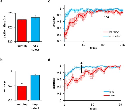
Behavioral performance. Group means for all participants and trials are shown here for (a) reaction time and (b) accuracy measures. (c) Average learning curves show accuracy (proportion correct) as a function of trial number for both task types (see legend for color assignment). At 100 trials (marked with a bar), learning performance reached asymptote. In (d), the number of trials was restricted to the cutoff from (c) and divided into fast and slow learners (see Figure 3 for details) for associative learning only. [Color figure can be viewed at http://wileyonlinelibrary.com.]

Rate Parameter Estimation

Each individual had a unique trajectory for acquiring new associations (Fig. 3). Based on average behavioral performance obtained from comparing response selection to associative learning tasks (Fig. 2c), only the first 100 trials were considered the active period. An exponential function was fit to individual accuracy curves to calculate the rate of acquisition. Goodness‐of‐fit indices (Table 1) indicated high r‐square values, low RMSE, and tight confidence intervals for 13 out of 14 participants only for the smoothing factor of 10 trials. For learner 8, however, a negative r‐square value was obtained. Given that r‐square is defined as the proportion of variance accounted for by the fit; in the event that the fit is poor, a negative r‐square value can be possible. The fit can be poor due to two probable reasons: an inappropriate starting point for the iterative fit or the lack of a constant term in the exponential equation being used for fitting. The choice of the exponential function was based on previous application in the context of learning [Buchel et al., 1999] and because this function was successful in fitting data from 13 out of 14 participants, we examined more closely the starting point of the fit and the smoothing parameters that data had undergone as an initial data processing step. Learner 8 had the best fit for a smoothing factor of 6 trials, which did not change dramatically the rate but boosted the r‐square value by a large margin (see a in Table 1), possibly because the starting value for the fit was more appropriate in this case and there were less outliers to fit compared to the scenario with smoothing by 10 trials. Rather than discount this participant's data, we kept the initial smoothing option of 10 trials. The rate parameter was rounded to two decimal places for learner 8 for all subsequent calculations. By making this assumption, fair comparisons between all participants' rate estimates could be made.

Learner Profiles

Neuropsychological test data were analyzed with PCA to uncover commonalities among test types and to reduce data dimensions. The scree plot and Kaiser's rule corroborated retention of the first three PCs which in total accounted for 84% of the variance. Correlations between the original variables and the component scores are shown in Figure 4a. A cutoff of 0.7 (almost half of the variance in the original variable accounted for by the component) was applied. The first PC grouped phonemic word generation, forward and backward digit span tests. These tests tend to rely on maintenance in working memory. Only two tests, both involving verbal memory where semantic details are retained over short and long delays, were expressed in the second PC. The last component was indicative of visual and spatial ability since the design tests and the sequence digit span required complex manipulation of visual/spatial material in memory.

Figure 4.

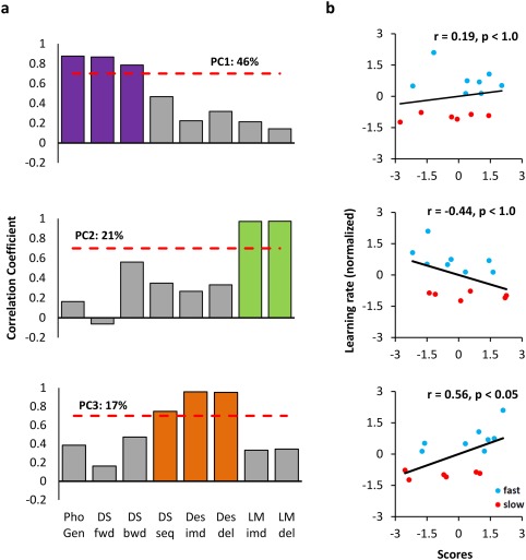
Principal components and their relationships with learning rate. (a) Component loadings for the first three principal components at the 0.7 cutoff (red line). At this mark, more than half of the variable's variance is explained by the component. Colored bars show the variables that surpass threshold; all other bars are in gray. Different aspects of memory—working (purple), verbal (green), and visual/spatial (orange)—are emphasized in each component. For further details about individual test categories, see Supporting Information, Table S1. (b) Scatterplots depict the relationship between learning rate (y‐axis) and scores for each component. The correlation coefficient (r) and the P value (obtained from permutation testing) are also displayed above each plot. Scatterplots show differentiation by group: fast (blue) and slow (red). [Color figure can be viewed at http://wileyonlinelibrary.com.]

Next, the component scores were correlated with the rate parameter as a continuous measure (Fig. 4b). There was a strong positive relationship (r = 0.56) between the speed of learning and the third PC (scatter plot is shown in Fig. 4b). This positive correlation was the only one that passed permutation testing (P < 0.05) and was also reliable across participants (95% confidence bounds: [0.093 0.832]).

Group Differences in Spatiotemporal Activity

When the average estimate of rate (k = 0.12) for the current participant sample was calculated, it was obvious that participants either acquired associations fairly quickly (bottom panel, Fig. 3; fast means: 0.19 ± 0.02 [standard error of the mean]) or relatively slowly (top panel, Fig. 3; slow means: 0.04 ± 0.01). Given these data, we divided participants into fast and slow groups rather than consider the rate of acquisition as a continuous variable. Average rates for fast and slow learners in the associative learning task are the only ones depicted in Figure 2d.

To investigate this trend in brain data, participants were assigned to two groups: fast and slow. Brain data was further divided into equal sets of trials sampling the learning process. This split was based on fast learners acquiring associations quickly (during first 33 trials, see Fig. 2d) after which point their performance accuracy was at ceiling. In slow learners, performance accuracy approached ceiling during later trials of learning (67–100 trials). By equating the behavioral performance in these two groups, we could uncover different neural strategies (network organizations) that corresponded to differences in behavioral performance (i.e., rate of acquisition). The middle set of trials was not considered here based on the assumption that there would be greater variations in brain responses in this period as slow learners explored different ways of acquiring the correct conditional associations. This exploratory phase (as seen by fluctuations in response accuracy) would make it challenging to find overlapping brain activity patterns across the slow group. On the other hand, performance of fast learners would have reached asymptote during the middle period, and therefore, learners within this group would possibly display more similar brain activity patterns. Due to greater individual variability in the slow group during the middle set of trials, a fair comparison between fast and slow learners would not be made if these trials were considered.

Hypothetically, two patterns could be present in the data—similar patterns of brain activity regardless of differences in behavioral performance for the two groups (fast vs slow) or differences in brain activity that corresponded to differences in behavior during the learning process (e.g., fast early vs slow late). The PLS analysis identified a single statistically significant latent variable (P < 0.05) that emphasized group differences in brain activity (fast vs slow). This latent variable accounted for 84% of the cross‐block covariance (Fig. 5a). Clusters that met spatiotemporal criteria are shown in Figure 5b (see figure caption for abbreviations). Group differences were expressed at several time points for all clusters (Fig. 5c). The full list of spatial locations in MNI coordinates (xyz in mm) corresponding to the cluster peaks from group analysis was as follows: GFi, inferior frontal gyrus [x: 36.0 y: 40.0 z: −8.0]; Cu, cuneus [x: 16.0 y: −92.0 z: 16.0]; PHG, parahippocampal gyrus [x: 20.0 y: −43.0 z: 6.0]; Caud, caudate head [x: 12.0 y: 20.0 z: 4.0]; LPi, inferior parietal lobule [x: −44.0 y: −32.0 z: 40.0]; LPp, posterior parietal [x: −40.0 y: −68.0 z: 40.0]; PCC, posterior cingulate cortex [x: −16.0 y: −56.0 z: 8.0]; PCu, precuneus [x: −20.0 y: −60.0 z: 24.0]; MTG, middle temporal gyrus [x: 64.0 y: −40.0 z: −4.0]; STG, superior temporal gyrus [x: 60.0 y: −4.0 z: 4.0]; GPrC, precentral gyrus [x: 56.0 y: 8.0 z: 12.0]; GPoC, postcentral gyrus [x: −44.0 y: −28.0 z: 44.0].

Figure 5.

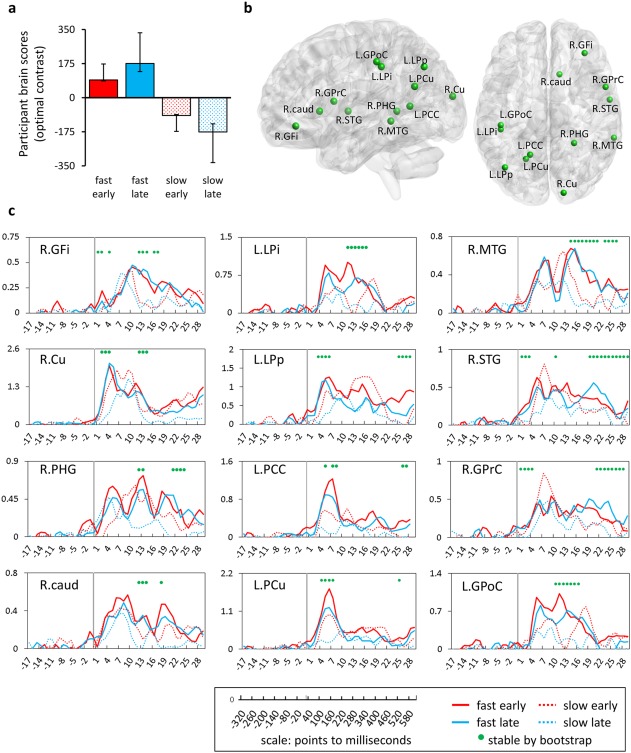
Spatiotemporal brain activity patterns for fast and slow learners. (a) and (b) outline the optimal contrast captured by the latent variable and its expression in different brain regions. (a) Contrast shows group differences in activations irrespective of learning stage (early, late). Error bars indicate confidence intervals (95%) derived from the bootstrap distribution. (b) MEG sources that reliably expressed the contrast are visualized with Brain Net Viewer [Xia et al., 2013] with spatial locations taken from cluster peaks from group analysis. Average source amplitudes (measured as pseudo‐z) for time ranges (points to millisecond conversion in legend) are displayed for each region in (c) with the baseline indicated as the period before the grey line (scene onset: 0 s). Time ranges where group differences were robustly expressed (absolute bootstrap ratio of greater than ± 2.5) are shown with green circles. Regions are labeled by hemisphere (L/R) and abbreviations are available in the text. [Color figure can be viewed at http://wileyonlinelibrary.com.]

Fast learners engaged some regions (R GFi, R Cu, L LPp, R STG) earlier in the trial compared to slow learners. For other regions (R MTG, R STG, R GPrC), the amplitude was greater for fast learners later in the trial. Notably, inferior frontal (R GFi), medial temporal (R PHG), and striatal areas were more active in fast learners during the middle of the trial. Also, these regions shared many time points where the group difference was expressed reliably as indicated by the BSR. As anticipated, spatiotemporal patterns were complex and reflected transient network configurations that took place within trials. However, we did notice that there were distinct times within the trial where brain responses were changing (see Supporting Information, Fig. S2 for graph). Generally, brain scores are collapsed across space and time, but by plotting participant brain scores on a timepoint‐by‐timepoint basis, we noted that brain responses changed within the scene encoding period in increments of 200 ms. Therefore, these time bins were chosen for subsequent connectivity analyses (see next section).

Network Organization at Multiple Time Scales

The regions that were selected in the first PLS were sensitive to group differences in acquiring novel associations. Time series from these spatial locations (Fig. 5b) served as the input for network analysis at multiple time scales (ms/min). Correlation matrices were computed for 6 conditions in total: 2 groups (fast and slow) and 3 bins (approximately 200 ms in length) within the trial representing the millisecond time range. To get the average connectivity matrices, participant correlation data was subjected to a Fisher transformation [Fisher, 1915]. This procedure normalizes correlations that lie near the extremes (±1) [Fisher, 1921]. The transformed data was averaged and then a reverse transform was computed to obtain the mean correlation values.

Out of the four pairwise analyses computed, only one analysis with fast learners using the first block of trials and the slow learners using the last block of trials within the active learning period was significant (P < 0.05). We examined behavioral performance during these trials for both groups and found that there was considerable overlap in the error bars (standard error of the mean); although we could not calculate an accurate rate given the decrease in data points from 100 to 33 (Fig. 6a). The group/condition effect captured by the latent variable showed an interaction between group assignment (fast early, slow late) and time segments during scene encoding; and accounted for 39% percent of the cross‐block covariance (Fig. 6b). The contrast illustrated in Figure 6a was expressed in stable functional connectivity patterns that were thresholded at 95% confidence bound from bootstrapping procedures (Fig. 6c). The strength and direction of connections were retrieved from the original group‐average correlation matrices for each condition (Fig. 6d).

Figure 6.

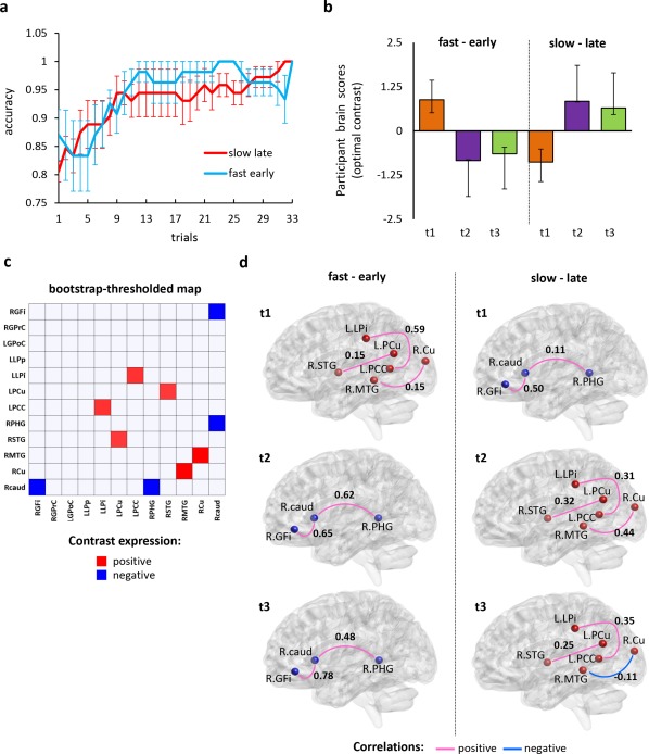
Functional connectivity dynamics by learning stage and group assignment. (a) Preasymptotic performance, indexed by the shape of accuracy curve and overlap in error bars (standard error of the mean), is displayed for the early trials during the learning session for the fast group (blue) and the late set of trials for the slow group (red). (b) PLS identified a significant latent variable that captures an interaction effect between groups (fast and slow) and time bins within a trial (t1–3). (c) Robust expression of the PLS contrast (absolute bootstrap ratio >2) are plotted in matrix format with sources in the rows and columns. Source names follow the convention reported in Figure 5. (d) Positive (red circles) and negative (blue) expressions of the contrast in (b) are visualized with Brain Net Viewer [Xia et al., 2013]. Strength and direction of stable correlations are shown using values and pink/light blue lines. [Color figure can be viewed at http://wileyonlinelibrary.com.]

Functional connections that fast learners recruited early in the trial epoch were the same connections that slow learners recruited late in the trial epoch. For fast learners, the correlation between L PCC and L LPi was strongest (r = 0.59) at early time bins (first 200 ms) but for slow learners, posterior regions were functionally connected (r > 0.3) and the strongest connection was between L Cu and MTG (r = 0.44) in the second time bin (200–400 ms). By the third time bin (400–600 ms), the slow learners also showed higher functional connectivity between L LPi and L PCC (r = 0.35), similar to the fast learners in first time bin (0–200 ms).

Fast learners engaged the same functional connections in the latter two‐thirds of the trial (time bins 2 and 3) as the slow learners in the first third of the trial (time bin 1). Three regions—R GFi, R caud, and R PHG—were positively coupled for fast learners in time bin 2. In time bin 3, coupling between R GFi and R caud increased (from r = 0.65 to r = 0.78) and this was paralleled by a decrease in coupling between R PHG and R caud (from r = 0.62 to r = 0.48). For slow learners, R GFi was positively correlated with R caud (r = 0.5) and R caud and R PHG shared a weak positive correlation (r = 0.11).

Brain–Behavior Relationships

To more directly assess whether the recruitment of a certain network configuration at a specific time in the learning trial could be predicted from independent scores cognitive ability, a post‐hoc analysis was performed (Fig. 7). Note that the third principal component derived from PCA had a positive correlation with the rate of acquisition (Fig. 4b, last row). Scores on this component were correlated with participant brain scores reflecting the positive and negative expression of the contrast in Figure 6 (e.g., functional connectivity dynamics). There was a positive correlation (r = 0.60, P < 0.05 – determined from permutation testing) between the network connectivity in posterior regions (referred to as the posterior network) and visuospatial ability (Fig. 7a) for fast learners in time bin 1 and slow learners in time bin 3 (positive expression of the contrast in Fig. 6b). There was no correlation between network connectivity in prefrontal, striatal, and medial temporal areas (referred to as the memory network) and visuospatial skill (Fig. 7b) for fast learners in time bin 3 and slow learners in time bin 1 (negative expression of the contrast in Fig. 6b).

Figure 7.

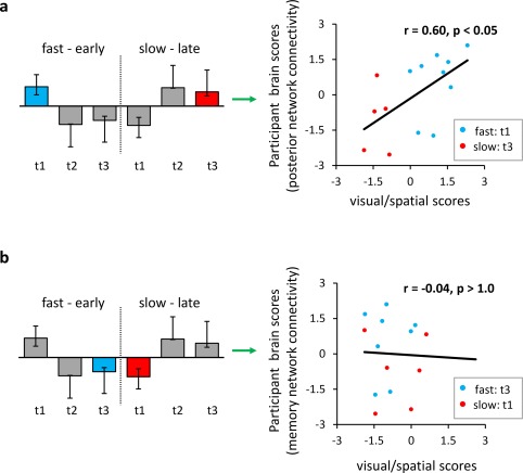
Functional connectivity dynamics and cognitive ability. Previously, functional connectivity in each group was assessed at three consecutive time bins within a trial (t1: 0–200 ms, t2: 200–400 ms, t3: 400–600 ms) with PLS (Fig. 6b). The main latent variable was characterized by increased connectivity within the posterior memory network in time bin 1 for fast learners (blue bar) and time bin 3 for slow learners (red bar), compared to the connectivity within the associative memory network in time bin 3 for fast learners (blue bar) and time bin 1 for slow learners (red bar; see Fig. 6d for details). Here, participant scores (extent to which participant's connectivity data expresses the latent variable in Fig. 6d) against cognitive scores from neuropsychological tests. (a) Participant scores associated with increased connectivity in the posterior memory network are correlated with visual/spatial scores derived from the third principal component (see Fig. 4b, last row). (b) Participant scores associated with decreased connectivity in the associative memory network are correlated with visual/spatial scores derived from the third principal component. Correlation coefficients (r) and p values are indicated on scatterplots. [Color figure can be viewed at http://wileyonlinelibrary.com.]

DISCUSSION

The majority of neuroimaging studies on human learning have focused on examining hemodynamic activity at coarse time scales (seconds) in several regions including medial temporal, striatal, and prefrontal regions [Poldrack et al., 1999, 2001; Toni and Passingham, 1999; Hartley et al., 2003; Iaria et al., 2003; Voermans et al., 2004; Law et al., 2005; Moses et al., 2010; Sadeh et al., 2010; Mattfeld and Stark, 2011]. In some of these experiments, strategic differences between individuals performing a task have been explored in selected regions that comprise memory networks [Iaria et al., 2003; Law et al., 2005; Mattfeld and Stark, 2011; Sanfratello et al., 2014]. More recently [Bassett et al., 2015], learning‐related changes have been studied in large‐scale functional networks for multiple timescales (resolution of seconds) and practice sessions (blocks, days). Here we expand on this work in several ways. First, we show that dynamic changes in functional networks occur at even finer temporal resolutions (milliseconds) afforded by MEG. Second, these dynamic functional configurations are related to cognitive ability and online performance during associative learning.

Distributed Spatiotemporal Activity

Our findings suggest that large‐scale network activity changes throughout associative learning (Fig. 5b). Particularly, two features mark individual differences in rate of change of behavioral performance. First, fast learners had greater activity in a specific subset of areas (R GFi, L LPi, R MTG, R STG, R GPrC, and L GPoC) at specific times in the trial compared to slow learners. Second, the onset of activity was earlier in the trial for the fast group in the same or other regions (R GFi, R Cu, L LPp, and R STG). Given that the data‐driven contrast (Fig. 5a) expressed group differences, magnitude increases and earlier activity onsets could be related to any part of the learning session (early or late trials). Previous research shows that increased activity in some regions (e.g., anterior cingulate, posterior parietal, medial prefrontal cortex, cerebellum, etc., see table in Kelly and Garavan [2005] for full list) was found in early learning where participants directed greater attention to new information [Kelly and Garavan, 2005]; whereas, temporal shifts arose from anticipatory (priming) responses that developed as a result of learning [Nobre et al., 2007]. In our data, these characteristics jointly distinguish fast performers from slower ones.

Whole‐brain analysis also revealed coincident activity in medial temporal (R PHG), striatal (R caud), and prefrontal (R GFi) areas for individuals that acquired associations quickly. This is significant because previous work has suggested that medial temporal and striatal regions engage in a competitive relationship [Poldrack and Packard, 2003] and that their interactions are likely mediated by prefrontal cortices [Poldrack et al., 2001]. By contrast, our data demonstrate transient (last a few hundred milliseconds) and time‐dependent co‐activations. We speculate that in past fMRI studies, this cooperative effect may have been attenuated due to the poor temporal resolution of the method. To our knowledge, this is the first demonstration of transient activity in these regions related to associative learning.

Time‐Dependent Functional Connectivity

The functional connectivity analysis was geared toward linking behavioral changes (fast/slow trajectories) over longer time scales (early/late parts of the learning session) to neural changes occurring at short timescales (three periods of 200 ms each within the trial). A latent variable (Fig. 6b) indicating a three‐way interaction (group by learning phase by time bin) was significant. To interpret this pattern, trial‐by‐trial accuracy plots were re‐examined. It was apparent that both groups displayed similar behavior (overlapping error bars) in the pre‐asymptotic phase, i.e., behavioral trajectories showed incremental gains in acquiring associative relationships. In terms of brain responses, however, unique network configurations were identified at separate times in the trial.

Fast performers engaged a posterior network that consisted of posterior cingulate (L PCC), precuneus (L PCu), inferior parietal (L LPi), middle temporal (R MTG), and cuneus (R Cu) regions during early scene processing (0–200 ms). Interactions within this posterior network could be necessary for representing spatial and topographical aspects of the scene. Support for this claim comes from patients with posterior cortical atrophy who show profound impairments in visuospatial processing [Gardini et al., 2011]. Within this network, strongest functional coupling (high correlation) was present for inferior parietal (L LPi) and posterior cingulate (L PCC) cortices. Inferior parietal areas have been implicated in coding spatial relations [Suchan et al., 2002]. Interestingly, emerging ideas about the functional contribution of the posterior cingulate suggest that this region may interface with learning systems in the brain to detect changes in the environment and to adapt responses to meet external demands [Pearson et al., 2011]. Since feedback in the task is not provided until after responses are made, greater connectivity between these regions could reflect maintenance of visuospatial content of scenes for informing later behavioral choices. During latter parts of the trial (200–600 ms), positive functional relationships were seen among medial temporal (R PHG), dorsal striatal (R caud), and ventrolateral prefrontal (R GFi) areas. These data suggest that the coactivity patterns observed in the group analysis (Fig. 5b) did indeed reflect interactions among learning and memory systems in the fast group.

Slow performers relied on prefrontal–striatal regions early in the trial but functional coupling between medial temporal and striatal areas was weak. Considering that spatial elements of the scene are extracted in later parts of the trial for slow learners (posterior sites are functionally coupled late), the medial temporal areas may not be engaged for binding elements together [Olsen et al., 2012]. This role may at least partly be fulfilled by sensory regions such as the cuneus (R Cu). The coupling between cuneus (R Cu) and middle temporal gyrus (R MTG), another area involved in visuospatial imagery [Pearson et al., 2011], was strongest during the middle part of the trial. Thus, the inference is that slow performers rely on visual imagery, for example, by actively imagining the spatial content of scenes during the task, rather than binding relations among spatial elements for later retrieval using medial temporal structures [Olsen et al., 2012]. Evidence for the importance of visual areas to conditional associative learning has been documented in nonhuman primates [Petrides, 1987]. Furthermore, there is some suggestion in humans that visual cues are recognized faster as a product of visuomotor learning [Toni and Passingham, 1999]. This strategy may be less efficient possibly because the same extrastriate region is not only registering the stimulus but also integrating spatial components. The bottleneck in visual areas can result in slower reaction times in sensorimotor tasks [Fatima and McIntosh, 2011] and may be responsible for less efficiency in task performance here.

In sum, the functional connectivity analysis demonstrated that even when slow learners were performing well (late stage), their network organization was different from fast learners. Although both network strategies supported acquisition of novel associations, the features that made each network different were the connection strengths among regions and the temporal order of when the functional interactions took place during a trial. But what makes an individual rely on one network configuration versus another to perform this task? Were there inherent differences in the cognitive abilities of individuals? To answer these questions, we used normative data acquired via a small battery of neuropsychological tests and linked it to behavioral performance in the associative learning task.

Cognitive Ability and Online Behavioral Performance

Emerging trends in neuropsychological research implicate more than one neural mechanism for behavioral success [Merhav et al., 2015; Ryan et al., 2013; Smith et al., 2014; Voermans et al., 2004]. In our work, in spite of observing variable speeds of learning, all participants were able to acquire the full set of stimulus pairings before the end of the experimental session. We sought to examine whether there existed cognitive markers that could predict an individual's behavioral trajectory during associative learning and thereby the underlying network configuration. Such predictors of individual differences would be of utmost importance in customizing programs that reinstate brain function for persons with disease/disability.

A systematic data‐driven approach was used to test combinations of features across cognitive, behavioral, and neurophysiological domains. First, learner profiles were derived based on the relationship between certain cognitive skills, as measured by standardized neuropsychological batteries and online behavioral performance during learning. Rather than comparing each test to the learning rate measure, a data summary technique (PCA) [Abdi and Williams, 2010; McIntosh and Misic, 2013] was initially applied to quantify interdependencies between test types. Cognitive scores were summarized into three PCs, but only one of these components showed a statistically reliable relationship with the rate of behavioral change during associative learning (Fig. 4). The subtests that contributed to this factor were in the areas of visuospatial memory and complex manipulation of items in working memory. It seemed that participants with superior visuospatial working memory were also the ones that acquired associations at a faster pace.

Notably, sequence digit span considered as a working memory test [Wechsler, 2008] did not contribute to the first PC which contained high loadings from the forward and backward span versions. It is questionable whether the forward and backward digit span tests are indeed comparable in their extraction of working memory reserve [Reynolds, 1997]. Here, results suggest that forward and backward digit spans were more similar to each other than to the sequence subtest presumably because participants only had to repeat digits maintained in working memory. On the other hand, digit span sequence required participants to simultaneously maintain and manipulate items by repeating them in ascending order. This subtest was perhaps more challenging than its forward/backward counterparts. By the same token, the designs subtest was also demanding because participants had to maintain and manipulate visuospatial content across a short (immediate) or long delay. In the associative learning task, individuals remembered spatial relations within a scene over a delay period and retrieved the correct associative relationship with color at the time of target presentation. The cognitive strategies needed to do well in both designs and sequence digit span seemed to also be relevant for acquiring novel associations quickly. By using PCA and correlation analysis, we quantified the relationship between neuropsychological tests and task‐related performance.

Analysis of the normative data and the neuroimaging findings were necessary for understanding differences between fast and slow performers during associative learning from both a cognitive and a neural perspective. Fast learners likely have better visuospatial memory (higher correlations with learning rate, Fig. 4b, bottom right) and are thus able to remember which scene was presented on a given trial with incorrect feedback. Not only are fast performers able to retrace their steps after feedback, they also understand that there is a conditional association between the scene and color, as determined from the debriefing interview. Slow learners try many other strategies before they realize there is a conditional relationship and this could be in part due to the limits of their visuospatial memory (lower correlations with learning rate).

Cognitive Ability and Dynamic Network Organization

A final brain–behavior analysis was performed to link visuospatial memory ability and time‐dependent network connectivity. This analysis was performed by taking cognitive scores from the third principal component and correlating them with brain scores from the functional connectivity analysis. Results revealed that connectivity within the posterior memory network was positively related to cognitive scores on visuospatial working memory subtests which were in turn positively correlated with learning rate. In other words, faster learning of novel associations could be predicted from better visuospatial ability and early engagement of posterior regions.

Surprisingly, there were no statistically reliable cognitive predictors of online behavioral performance or time‐dependent changes in the associative memory network. It may be the case that the visuospatial scores captured by the neuropsychological subtests administered here were not sufficient for capturing features of the associative memory network. By increasing the variety of cognitive tests and the data sample, maybe such relationships can be delineated in future studies.

CONCLUSIONS

Here, we used MEG to examine network dynamics at fast timescales (millisecond resolution) and their links to behavioral outcomes across a learning session (minute resolution). By applying a fully data‐driven multivariate approach, we obtained comprehensive measures of network‐level interactions, behavioral performance and cognitive ability. This study extends previous amplitude‐based findings in several ways. First, it shows that large‐scale networks interact at multiple time scales and can support individual differences in learning (fast and slow) by mitigating the temporal order, the strength, and the direction of their connections. Second, typically, empirical studies relate neural activity patterns without temporal specificity (within a trial or across the learning session) to behavioral data from neuropsychological tests. Here, we show that the timing and connectivity within subnetworks relate uniquely to cognitive skills assessed using these tests. Last, interindividual differences in the timing of network interactions are largely ignored in experiments that emphasize group averages. These temporal changes in learning may be critical for understanding variability in neural, cognitive, and behavioral responses across people.

At present, large databases that conglomerate information about neuropsychological tests, behavioral performance during different tasks, and neurophysiological data are becoming increasingly popular [Van Horn et al., 2005]. However, in clinical practice, neuropsychological assessments still remain the gold standard for assessing cognitive deficits [Harvey, 2012]. The data‐driven approaches described here can potentially be employed in mining neuroimaging databases to find unique clusters of individuals that have defining attributes in several domains: cognitive, behavior, and neural network organization. Eventually, this information can take the form of normative databases that can classify new individuals in terms of pre‐existing cognitive and neural profiles. Such normative databases can perhaps change the landscape of rehabilitative medicine by systematically catering to individual differences in cognitive abilities.

FUNDING

This work was supported by a graduate scholarship from Ontario Mental Health Foundation to ZF. The authors declare that there are no conflicts of interest.

Supporting information

Supporting Information

REFERENCES

- Abdi H, Williams LJ (2010): Principal component analysis. Wiley Interdisc Rev Comput Stat 2:433–459. [Google Scholar]
- Allen EA, Damaraju E, Plis SM, Erhardt EB, Eichele T, Calhoun VD (2014): Tracking whole‐brain connectivity dynamics in the resting state. Cereb Cortex 24:663–676. [DOI] [PMC free article] [PubMed] [Google Scholar]
- Bassett DS, Wymbs NF, Porter MA, Mucha PJ, Carlson JM, Grafton ST (2011): Dynamic reconfiguration of human brain networks during learning. Proc Natl Acad Sci USA 108:7641–7646. [DOI] [PMC free article] [PubMed] [Google Scholar]
- Bassett DS, Yang M, Wymbs NF, Grafton ST (2015): Learning‐induced autonomy of sensorimotor systems. Nat Neurosci 18:744–751. [DOI] [PMC free article] [PubMed] [Google Scholar]
- Braver TS, Cole MW, Yarkoni T (2010): Vive les differences! Individual variation in neural mechanisms of executive control. Curr Opin Neurobiol 20:242–250. [DOI] [PMC free article] [PubMed] [Google Scholar]
- Bressler SL, Tognoli E (2006): Operational principles of neurocognitive networks. Int J Psychophysiol 60:139–148. [DOI] [PubMed] [Google Scholar]
- Brovelli A, Chicharro D, Badier JM, Wang H, Jirsa V (2015): Characterization of cortical networks and corticocortical functional connectivity mediating arbitrary visuomotor mapping. J Neurosci 35:12643–12658. [DOI] [PMC free article] [PubMed] [Google Scholar]
- Buchel C, Coull JT, Friston KJ (1999): The predictive value of changes in effective connectivity for human learning. Science 283:1538–1541. [DOI] [PubMed] [Google Scholar]
- Cheung MJ, Kovacevic N, Fatima Z, Misic B, McIntosh AR (2016): [MEG]PLS: A pipeline for MEG data analysis and partial least squares statistics. Neuroimage 124:181–193. [DOI] [PubMed] [Google Scholar]
- Delorme A, Makeig S (2004): EEGLAB: an open source toolbox for analysis of single‐trial EEG dynamics including independent component analysis. J Neurosci Methods 134:9–21. [DOI] [PubMed] [Google Scholar]
- Di X, Biswal BB (2015): Dynamic brain functional connectivity modulated by resting‐state networks. Brain Struct Funct 220:37–46. [DOI] [PMC free article] [PubMed] [Google Scholar]
- Diaconescu AO, Alain C, McIntosh AR (2011): The co‐occurrence of multisensory facilitation and cross‐modal conflict in the human brain. J Neurophysiol 106:2896–2909. [DOI] [PubMed] [Google Scholar]
- Duzel E, Habib R, Schott B, Schoenfeld A, Lobaugh N, McIntosh AR, Scholz M, Heinze HJ (2003): A multivariate, spatiotemporal analysis of electromagnetic time‐frequency data of recognition memory. Neuroimage 18:185–197. [DOI] [PubMed] [Google Scholar]
- Efron B, Tibshirani R (1986): Bootstrap methods for standard errors, confidence intervals and other measures of statistical accuracy. Stat Sci 1:54–77. [Google Scholar]
- Fatima Z, McIntosh AR (2011): The interplay of cue modality and response latency in brain areas supporting crossmodal motor preparation: an event‐related fMRI study. Exp Brain Res 214:9–17. [DOI] [PubMed] [Google Scholar]
- Fatima Z, Quraan MA, Kovacevic N, McIntosh AR (2013): ICA‐based artifact correction improves spatial localization of adaptive spatial filters in MEG. Neuroimage 78C:284–294. [DOI] [PubMed] [Google Scholar]
- Fisher RA (1915): Frequency distribution of the values of the correlation coefficient in samples of an indefinitely large population. Biometrika 10:507–521. [Google Scholar]
- Fisher RA (1921): On the 'probable error' of a coefficient correlation deduced from a small sample. Metron 1:3–32. [Google Scholar]
- Friston KJ (1995): Functional and effective connectivity in neuroimaging: a synthesis. Human Brain Mapping 2:56–78. [Google Scholar]
- Fu Z, Di X, Chan SC, Hung YS, Biswal BB, Zhang Z (2013): Time‐varying correlation coefficients estimation and its application to dynamic connectivity analysis of fMRI. Conf Proc IEEE Eng Med Biol Soc 2013:2944–2947. [DOI] [PubMed] [Google Scholar]
- Gardini S, Concari L, Pagliara S, Ghetti C, Venneri A, Caffarra P (2011): Visuo‐spatial imagery impairment in posterior cortical atrophy: a cognitive and SPECT study. Behav Neurol 24:123–132. [DOI] [PMC free article] [PubMed] [Google Scholar]
- Good P. 2000. Permutation Tests: A Practical Guide to Resampling Methods for Testing Hypotheses. New York: Springer. [Google Scholar]
- Gross J, Baillet S, Barnes GR, Henson RN, Hillebrand A, Jensen O, Jerbi K, Litvak V, Maess B Oostenveld R, et al. (2013): Good practice for conducting and reporting MEG research. Neuroimage 65:349–363. [DOI] [PMC free article] [PubMed] [Google Scholar]
- Handwerker DA, Roopchansingh V, Gonzalez‐Castillo J, Bandettini PA (2012): Periodic changes in fMRI connectivity. Neuroimage 63:1712–1719. [DOI] [PMC free article] [PubMed] [Google Scholar]
- Hartley T, Maguire EA, Spiers HJ, Burgess N (2003): The well‐worn route and the path less traveled: distinct neural bases of route following and wayfinding in humans. Neuron 37:877–888. [DOI] [PubMed] [Google Scholar]
- Harvey PD (2012): Clinical applications of neuropsychological assessment. Dialogues Clin Neurosci 14:91–99. [DOI] [PMC free article] [PubMed] [Google Scholar]
- Hopf L, Quraan MA, Cheung MJ, Taylor MJ, Ryan JD, Moses SN (2013): Hippocampal lateralization and memory in children and adults. J Int Neuropsychol Soc 19:1042–1052. [DOI] [PubMed] [Google Scholar]
- Hutchison RM, Womelsdorf T, Allen EA, Bandettini PA, Calhoun VD, Corbetta M, Della Penna S, Duyn JH, Glover GH Gonzalez‐Castillo J, and others. (2013): Dynamic functional connectivity: Promise, issues, and interpretations. Neuroimage 80:360–378. [DOI] [PMC free article] [PubMed] [Google Scholar]
- Iaria G, Petrides M, Dagher A, Pike B, Bohbot VD (2003): Cognitive strategies dependent on the hippocampus and caudate nucleus in human navigation: Variability and change with practice. J Neurosci 23:5945–5952. [DOI] [PMC free article] [PubMed] [Google Scholar]
- Jolliffe IT. 2002. Principal Component Analysis, 2nd ed New York: Springer. [Google Scholar]
- Kelly AM, Garavan H (2005): Human functional neuroimaging of brain changes associated with practice. Cereb Cortex 15:1089–1102. [DOI] [PubMed] [Google Scholar]
- Lalancette M, Quraan M, Cheyne D (2011): Evaluation of multiple‐sphere head models for MEG source localization. Phys Med Biol 56:5621–5635. [DOI] [PubMed] [Google Scholar]
- Law JR, Flanery MA, Wirth S, Yanike M, Smith AC, Frank LM, Suzuki WA, Brown EN, Stark CE (2005): Functional magnetic resonance imaging activity during the gradual acquisition and expression of paired‐associate memory. J Neurosci 25:5720–5729. [DOI] [PMC free article] [PubMed] [Google Scholar]
- Luck SJ, Vogel EK (2013): Visual working memory capacity: From psychophysics and neurobiology to individual differences. Trends Cogn Sci 17:391–400. [DOI] [PMC free article] [PubMed] [Google Scholar]
- Mattfeld AT, Stark CE (2011): Striatal and medial temporal lobe functional interactions during visuomotor associative learning. Cereb Cortex 21:647–658. [DOI] [PMC free article] [PubMed] [Google Scholar]
- McIntosh AR (2000): Towards a network theory of cognition. Neural Netw 13:861–870. [DOI] [PubMed] [Google Scholar]
- McIntosh AR, Bookstein FL, Haxby JV, Grady CL (1996): Spatial pattern analysis of functional brain images using partial least squares. Neuroimage 3:143–157. [DOI] [PubMed] [Google Scholar]
- McIntosh AR, Lobaugh NJ (2004): Partial least squares analysis of neuroimaging data: Applications and advances. Neuroimage 23:S250–S263. [DOI] [PubMed] [Google Scholar]
- McIntosh AR, Misic B (2013): Multivariate statistical analyses for neuroimaging data. Annu Rev Psychol 64:499–525. [DOI] [PubMed] [Google Scholar]
- McIntosh AR, Vakorin V, Kovacevic N, Wang H, Diaconescu A, Protzner AB (2013): Spatiotemporal dependency of age‐related changes in brain signal variability. Cereb Cortex 24:1806–1817. [DOI] [PMC free article] [PubMed] [Google Scholar]
- Merhav M, Karni A, Gilboa A (2015): Not all declarative memories are created equal: Fast Mapping as a direct route to cortical declarative representations. Neuroimage 117:80–92. [DOI] [PubMed] [Google Scholar]
- Mills T, Lalancette M, Moses SN, Taylor MJ, Quraan MA (2012): Techniques for detection and localization of weak hippocampal and medial frontal sources using beamformers in MEG. Brain Topogr 25:248–263. [DOI] [PubMed] [Google Scholar]
- Misic B, Mills T, Taylor MJ, McIntosh AR (2010): Brain noise is task dependent and region specific. J Neurophysiol 104:2667–2676. [DOI] [PubMed] [Google Scholar]
- Misic B, Mills T, Vakorin VA, Taylor MJ, McIntosh AR (2014): Developmental trajectory of face processing revealed by integrative dynamics. J Cogn Neurosci 26:2416–2430. [DOI] [PubMed] [Google Scholar]
- Moses SN, Ryan JD, Bardouille T, Kovacevic N, Hanlon FM, McIntosh AR (2009): Semantic information alters neural activation during transverse patterning performance. Neuroimage 46:863–873. [DOI] [PMC free article] [PubMed] [Google Scholar]
- Moses SN, Brown TM, Ryan JD, McIntosh AR (2010): Neural system interactions underlying human transitive inference. Hippocampus 20:894–901. [DOI] [PubMed] [Google Scholar]
- Nobre A, Correa A, Coull J (2007): The hazards of time. Curr Opin Neurobiol 17:465–470. [DOI] [PubMed] [Google Scholar]
- Olsen RK, Moses SN, Riggs L, Ryan JD (2012): The hippocampus supports multiple cognitive processes through relational binding and comparison. Front Hum Neurosci 6:146. [DOI] [PMC free article] [PubMed] [Google Scholar]
- Pearson JM, Heilbronner SR, Barack DL, Hayden BY, Platt ML (2011): Posterior cingulate cortex: Adapting behavior to a changing world. Trends Cogn Sci 15:143–151. [DOI] [PMC free article] [PubMed] [Google Scholar]
- Petrides M (1985): Deficits on conditional associative‐learning tasks after frontal‐ and temporal‐lobe lesions in man. Neuropsychologia 23:601–614. [DOI] [PubMed] [Google Scholar]
- Petrides M. 1987. Conditional learning and the primate frontal cortex In: Perecman E, editor. The Frontal Lobes Revisited. New York, N.Y: IRBN Press; p 91–108. [Google Scholar]
- Poldrack RA, Clark J, Pare‐Blagoev EJ, Shohamy D, Creso Moyano J, Myers C, Gluck MA (2001): Interactive memory systems in the human brain. Nature 414:546–550. [DOI] [PubMed] [Google Scholar]
- Poldrack RA, Packard MG (2003): Competition among multiple memory systems: Converging evidence from animal and human brain studies. Neuropsychologia 41:245–251. [DOI] [PubMed] [Google Scholar]
- Poldrack RA, Prabhakaran V, Seger CA, Gabrieli JD (1999): Striatal activation during acquisition of a cognitive skill. Neuropsychology 13:564–574. [DOI] [PubMed] [Google Scholar]
- Quraan MA, Cheyne D (2010): Reconstruction of correlated brain activity with adaptive spatial filters in MEG. Neuroimage 49:2387–2400. [DOI] [PubMed] [Google Scholar]
- Reynolds CR (1997): Forward and backward memory span should not be combined for clinical analysis. Arch Clin Neuropsychol 12:29–40. [PubMed] [Google Scholar]
- Riggs L, Moses SN, Bardouille T, Herdman AT, Ross B, Ryan JD (2009): A complementary analytic approach to examining medial temporal lobe sources using magnetoencephalography. Neuroimage 45:627–642. [DOI] [PubMed] [Google Scholar]
- Robinson SE, Vrba J. 1999. Recent advances in biomagnetism In: Yoshimoto T, Kotani M, Kuriki S, Karibe S, Nakasato N, editors. Functional Neuroimaging by Synthetic Aperture Magnetometry (SAM). Sendai, Japan: Tohoku University Press; p 302–305. [Google Scholar]
- Ryan JD, Moses SN, Barense M, Rosenbaum RS (2013): Intact learning of new relations in amnesia as achieved through unitization. J Neurosci 33:9601–9613. [DOI] [PMC free article] [PubMed] [Google Scholar]
- Sadeh T, Shohamy D, Levy DR, Reggev N, Maril A (2010): Cooperation between the hippocampus and the striatum during episodic encoding. J Cogn Neurosci 23:1597–1608. [DOI] [PubMed] [Google Scholar]
- Sanfratello L, Caprihan A, Stephen JM, Knoefel JE, Adair JC, Qualls C, Lundy SL, Aine CJ (2014): Same task, different strategies: How brain networks can be influenced by memory strategy. Hum Brain Mapp 35:5127–5140. [DOI] [PMC free article] [PubMed] [Google Scholar]
- Sato N, Nakamura K, Nakamura A, Sugiura M, Ito K, Fukuda H, Kawashima R (1999): Different time course between scene processing and face processing: A MEG study. Neuroreport 10:3633–3637. [DOI] [PubMed] [Google Scholar]
- Sekihara K, Nagarajan SS, Poeppel D, Marantz A, Miyashita Y (2001): Reconstructing spatio‐temporal activities of neural sources using an MEG vector beamformer technique. IEEE Trans Biomed Eng 48:760–771. [DOI] [PubMed] [Google Scholar]
- Smith CN, Urgolites ZJ, Hopkins RO, Squire LR (2014): Comparison of explicit and incidental learning strategies in memory‐impaired patients. Proc Natl Acad Sci USA 111:475–479. [DOI] [PMC free article] [PubMed] [Google Scholar]
- Spreng RN, Sepulcre J, Turner GR, Stevens WD, Schacter DL (2013): Intrinsic architecture underlying the relations among the default, dorsal attention, and frontoparietal control networks of the human brain. J Cogn Neurosci 25:74–86. [DOI] [PMC free article] [PubMed] [Google Scholar]
- Suchan B, Yaguez L, Wunderlich G, Canavan AG, Herzog H, Tellmann L, Homberg V, Seitz RJ (2002): Neural correlates of visuospatial imagery. Behav Brain Res 131:163–168. [DOI] [PubMed] [Google Scholar]
- Toni I, Passingham RE (1999): Prefrontal‐basal ganglia pathways are involved in the learning of arbitrary visuomotor associations: A PET study. Exp Brain Res 127:19–32. [DOI] [PubMed] [Google Scholar]
- Urbain CM, Pang EW, Taylor MJ (2015): Atypical spatiotemporal signatures of working memory brain processes in autism. Transl Psychiatry 5:e617. [DOI] [PMC free article] [PubMed] [Google Scholar]
- Van Horn JD, Wolfe J, Agnoli A, Woodward J, Schmitt M, Dobson J, Schumacher S, Vance B. (2005): Neuroimaging databases as a resource for scientific discovery International Review of Neurobiology. Academic Press; p 55–87. [DOI] [PubMed] [Google Scholar]
- Voermans NC, Petersson KM, Daudey L, Weber B, Van Spaendonck KP, Kremer HP, Fernandez G (2004): Interaction between the human hippocampus and the caudate nucleus during route recognition. Neuron 43:427–435. [DOI] [PubMed] [Google Scholar]
- Wechsler D. 2008. Wechsler Adult Intelligence Scale ‐ Fourth Edition. San Antonio, TX: Pearson. [Google Scholar]
- Wechsler D. 2009. Wechsler Memory Scale ‐ Fourth Edition. San Antonio, TX: Pearson. [Google Scholar]
- Xia M, Wang J, He Y (2013): BrainNet Viewer: a network visualization tool for human brain connectomics. PLoS One 8:e68910. [DOI] [PMC free article] [PubMed] [Google Scholar]
Associated Data
This section collects any data citations, data availability statements, or supplementary materials included in this article.
Supplementary Materials