Classification based hypothesis testing in neuroscience: Below‐chance level classification rates and overlooked statistical properties of linear parametric classifiers

Abstract

Multivariate pattern analysis (MVPA) has recently become a popular tool for data analysis. Often, classification accuracy as quantified by correct classification rate (CCR) is used to illustrate the size of the effect under investigation. However, we show that in low sample size (LSS), low effect size (LES) data, which is typical in neuroscience, the distribution of CCRs from cross‐validation of linear MVPA is asymmetric and can show classification rates considerably below what would be expected from chance classification. Conversely, the mode of the distribution in these cases is above expected chance levels, leading to a spuriously high number of above chance CCRs. This unexpected distribution has strong implications when using MVPA for hypothesis testing. Our analyses warrant the conclusion that CCRs do not well reflect the size of the effect under investigation. Moreover, the skewness of the null‐distribution precludes the use of many standard parametric tests to assess significance of CCRs. We propose that MVPA results should be reported in terms of P values, which are estimated using randomization tests. Also, our results show that cross‐validation procedures using a low number of folds, e.g. twofold, are generally more sensitive, even though the average CCRs are often considerably lower than those obtained using a higher number of folds. Hum Brain Mapp 37:1842–1855, 2016. © 2016 Wiley Periodicals, Inc.

INTRODUCTION

Multivariate pattern analysis (MVPA) is becoming more and more mainstream for classification, decoding, and hypothesis testing in neuroscientific data analysis [Damarla and Just, 2013; Deuker et al., 2013; Duarte, et al., 2014; Haynes and Rees, 2006; Kamitani and Tong, 2005; Norman et al., 2006; Staresina et al., 2013], with linear classifiers being the most successful ones [Clarke et al., 2008; Lemm et al., 2011]. Whereas classical statistical approaches search for one or more features in a data set that independently allow to distinguish between experimental conditions or groups, multivariate classification algorithms analyze data sets in a way that takes into account all the available information contained therein. Therefore, they provide increased sensitivity compared with classical methods, which are based on multiple univariate comparisons. Because a classifier is usually trained on one portion of the data and then validated on another, it provides an estimation of the generalizability of the learned classification rule and can thus be used for data‐driven exploratory analyses as well as for hypothesis‐driven testing. These properties make multivariate pattern classification an attractive analysis tool for the neurosciences, where experiments often generate large amounts of multivariate data [Kriegeskorte et al., 2009; Norman et al., 2006].

Performance of MVPA algorithms is frequently quantified in terms of correct classification rates (CCRs), which is defined as the percentage of correctly classified items. The most widely used algorithm for CCR estimation is cross‐validation [Hastie et al., 2001]. It has a low bias, is simple to implement [Kohavi, 1995] and has been used to estimate classification performance in many applications [Braga‐Neto and Dougherty, 2004; Lemm et al., 2011; Noirhomme et al., 2014]. Cross‐validation makes efficient use of all the available data by repeatedly partitioning data into complementary training and test subsets. Thus, this method is especially suitable when there are only few available samples. Because it strictly separates classifier training from error estimation, it avoids overfitting the classifier to the data set. It also precludes confirming in the same data the hypotheses generated by the classifier during training and thus prevents circularity [Kriegeskorte et al., 2009]. Although these characteristics in principle should guarantee the safe employment of classification with cross‐validation for hypothesis testing purposes, it produces only a point estimate of classification accuracy, and its relation to the size of the effect in question is unclear.

Beyond the CCR, we need the confidence interval or better still the distribution of this estimation. Variance of cross‐validated CCRs depends on classifier type, on experimental design parameters like sample size and data dimensionality, and on signal‐to‐noise ratio inherent in the data [Azuaje, 2003; Clarke et al., 2008; Dougherty, 2001; Raudys and Jain, 1991; Rodriguez et al., 2010]. Neuroscience data usually has a number of properties that cause classification accuracies to have particularly large variances. First, they frequently contain hundreds or thousands of features (e.g. number of voxels in fMRI studies, number of channels times number of frequency bins or time points in EEG recordings, number of genes in cDNA microarray studies, etc.), which leads to a phenomenon known as noise accumulation. Noise accumulation is the increasing difficulty to determine the centroid of data in a space with increasing dimensionality. Second, features often contain only a small amount of information, i.e. the signal‐to‐noise ratio or effect size is small and differences between classes are hard to detect. Third, although data sets often consist of large numbers of features, the number of samples is often on the order of tens, because it is practically limited by the number of subjects that can participate in a study and by the number of trials each subject can complete within a reasonable time [see Button et al., 2013 for a related discussion]. This again makes accurate estimation of class centroids problematic.

Although MVPA is getting more and more attention in neuroimaging, its intricacies are not yet completely understood. Often, higher CCRs are essentially interpreted as representing larger effects, generally without further taking the properties of the data (e.g. sample size, number of features) or the classifier into account. To investigate the reliability of MVPA results in hypothesis testing applications, we explore the properties of cross‐validated classification accuracies in typical neuroscientific data, which we model as low sample size/low effect size data (LSS‐LES). We use simulations and an analytical approach to describe the distribution of classification results with systematically varying sample size, effect size, and number of cross‐validation folds. From our findings we draw conclusions regarding the use of cross‐validation in MVPA with linear classifiers for hypothesis testing. Our findings show that cross‐validation in LSS‐LES data possesses some counterintuitive properties that can critically bias interpretation of findings. In particular, we show that CCRs should not be used to display or compare class differences, because a higher CCR does not necessarily represent a larger difference between classes if not all the properties of the data sets are comparable (sample size, number of features, number of trials, type of cross‐validation, covariance matrices, etc.)

METHOD AND RESULTS

Case Study: Classification of EEG Data

The main premise of classification is that expected CCR of a given classifier has a monotonic, albeit nonlinear relation with the amount of signal in the data, i.e. classification of a data set with more information results in higher CCR [Raudys and Pikelis, 1980]. In particular, if the collected data from two experimental conditions represent identical distributions, i.e., the null hypothesis is true and thus the effect size is zero, one would expect CCRs near 50% (chance level). However, although this is true provided an asymptotically infinite number of samples, this does not seem to hold for low sample size data, which is usually available for hypothesis testing purposes. We noticed in the literature and in our own preliminary experiments that classification rates are often much lower than what could be expected even from chance performance, sometimes even approaching 0% [Deuker et al., 2013; Etzel et al., 2013; Fuentemilla et al., 2010; Gisselbrecht et al., 2013; Noirhomme et al., 2014]. These extreme below chance level CCRs are not generally matched by similarly high CCRs when an analysis is repeated multiple times within a series of analyses, which already hints at an asymmetry in the distribution of CCRs.

First, we consider the analysis of a study that aimed at investigating event related potentials (ERP) elicited by two kinds of visual stimuli in a visual learning task (see Fig. 1). In this experiment, EEG was recorded from 20 healthy subjects while two types of stimuli, which were photographs belonging to different semantic categories, were presented. Presentation time was 100 ms, the EEG was recorded from 100 ms before to 900 ms after onset of stimulus presentation. EEG was recorded using an active 128‐channel Ag/AgCl‐electrode system (ActiCap, Brain products, Gilching, Germany) with 1 kHz sampling frequency and a high‐pass filter of 0.1 Hz. Electrodes were placed according to the extended international 10–20 electrode system. Artifacts were rejected in a semiautomatic process using custom MATLAB scripts that made sure that only a minimal number of artifacts remained in the data. Epochs with artifacts were removed from the dataset, channels that contained too many epochs with artifacts were removed and then interpolated using routines provided by EEGLAB [Delorme and Makeig, 2004]. We used 30 artifact‐free trials of each stimulus category per subject for our within‐subject classification procedure. The goal of this study was to investigate whether and which aspects of the ERP in terms of spatial locations and time windows have discriminating power between the two types of stimuli. To answer this question, we used a so‐called searchlight approach [Kriegeskorte et al., 2006], sweeping the spatiotemporal feature space with a window size of 3 cm on‐scalp radius for spatial and 20 ms for temporal features, respectively, resulting in 1,600 searchlights with approximately 100 features on average. We classified the data in each searchlight with diagonal Linear Discriminant Analysis (LDA) using Leave‐One‐Out (LOO) cross‐validation. Figure 1b shows the histogram of CCRs for different searchlights for an exemplar subject. It becomes immediately obvious that this distribution has a heavy tail to the left, which is expected for neither zero nor positive effect sizes. To describe the distribution of CCRs quantitatively, we use three different measures: below chance percentage (BCP) denotes the percentage of results that have less than the chance level of 50% correct classifications. If the null hypothesis is true and CCRs are symmetrically distributed, 50% of below chance findings can be expected. A deviation from 50% indicates either a non‐zero effect (BCP > 50%) or a skewed distribution of CCRs (BCP < >50%). CCR_0.05 and CCR_0.95 represent the classification rates of the 5th and 95th percentile of the distribution. Although the average CCR is 52.7%, only about a quarter of CCRs fall below the expected chance level (BCP = 27.5%). On the other hand, the distribution shows a heavier tail on its left than its right side, i.e. below chance values are more extreme than above chance values. Together with the peak of the distribution (mode), which lies to the right of the mean at 55%, these data clearly demonstrate the asymmetry of distributions of classification outcomes: a few extremely low values are weighed against a higher number of above average values.

Figure 1.

Classification results in an EEG visual learning task. (A) A topo‐plot showing the standard electrode locations in high‐density EEG recording with four examples of average event‐related potentials from two frontal and two occipital channels. (B) Histogram of correct classification rates for 1,600 classifications using a searchlight procedure on spatiotemporal features of the EEG. The distribution shows a strong skewness with a heavy tail on the left.

Classification Rates Below the Level Expected for Chance

Using synthetically generated data, we have the opportunity to manipulate various parameters, we studied the actual shape of classification rate distributions in 21 series of 10,000 synthetically generated, one‐dimensional, two‐class experiments. Each simulated experiment consisted of $N=15$ observations per condition which were randomly sampled from two normally distributed populations. Populations had identical variances and a priori determined true effect sizes. The effect size is a measure of the amount of signal, here given as the mean difference between two classes in standard deviation units $\left(d=\frac{{\overline{x}}_1-{\overline{x}}_2}{\sqrt{\left({s_1}^2+{s_2}^2\right)/2}}\right)$. For the behavioral sciences, Cohen [1988] defined a value of $d=0.2$ as a small effect. We classified the data from each experiment using cross‐validation and LDA classification. For each particular true effect size, we repeated the whole sampling procedure 10,000 times.

We then pursued two complementary approaches to estimate the expected value of classification accuracies. In the first approach, we averaged over all the CCRs of those experiments that are generated from equal a priori, true effect size (Fig. 2a). In the second one, we averaged over CCRs of experiments with equal a posteriori, estimated effect sizes (Fig. 2b). Thus, we differentiate between the population‐based true effect size ( $d$) and the sample‐based estimated effect size ( $\widehat{d}$), which is observed in a specific finite sample. This is particularly relevant for any real data set, where we do not have access to the true effect size. Whereas intuitively, one may assume that expected CCRs are identical for true and estimated effect sizes, this turns out to be true only for large effect sizes. Our simulations on low sample size data exhibit large differences when effect sizes are small. We see in Figure 2a that expected values of CCRs start from chance level (here 50%) for a true effect size of $d=0$ and increase nonlinearly with increasing effect size. However, Figure 2b, which shows expected values of CCRs as a function of the observed, sample‐based effect sizes, demonstrates that average CCRs in low sample size data can drop far below 50% when the estimated effect size is low, which could explain the unexpectedly high number of very low CCRs around 20% in the empirical data in Figure 1b. In other words, classification of data sets with small estimated effect sizes results on average in below chance level CCRs. For the experiments simulated in Figure 2b, an estimated effect size of $\widehat{d}=0$ results in CCRs between 0% and 65%, and CCRs below 50% occur up to an effect size of $\widehat{d}=1$. This effect size represents a mean difference between conditions of one standard deviation and is already interpreted as a large effect in some fields [Cohen, 1988]. Only for even larger effects, expected CCRs for true and estimated effect sizes converge. We further investigated the distribution of estimated effect sizes and plot CCRs for all the experiments with an a priori true effect size of $d=0$. As expected, estimated effect sizes $\widehat{d}$ are symmetrically distributed around zero (Fig. 2c). However, CCRs follow another distribution which is neither normal nor binomial and not even symmetric (Fig. 2d). This observation shows that there is no simple relation between estimated effect size and CCR and that CCR therefore does not well reflect the size of the effect under study.

Figure 2.

Below chance classification rates in LSS‐LES data when classified using LDA with LOO cross‐validation. (A) Expected CCRs as a function of true effect size $d\in$ {0, 0.04, 0.08, 0.12, 0.16, 0.20, 0.24, 0.32, 0.44, 0.50, 0.6, 0.7, 0.8, 1, 1.2, 1.5, 2, 2.5, 3.5, 4, 5} provided infinite sample size. (B) The solid line shows the expected CCR as a function of the estimated effect size. Gray dots represent individual experiments. CCRs can only obtain discrete values. (C) Distribution of estimated effect sizes of experiments with a true effect size of zero. (D) Distribution of CCRs that result from experiments with a true effect size of zero. The gray area shows the experiments with classification rates below 50%.

The simulations in Figure 2 show that CCRs reach far below chance levels when sample size and estimated effect size is low. To further investigate the underlying causes of this observation, we develop an analytical description of cross‐validated classification rates in a one‐dimensional linear classification paradigm. We assume a data set that consists of $N$ observations for each of two classes $A$ and $B$ with empirical means $\overrightarrow{m}={\left[m_A,m_B\right]}^T$. During k‐fold cross‐validation the data set is divided into a training and a test set, with means $\overrightarrow{\mu } ={[\mu }_A,{\mu }_B]$ for the training set and $\overrightarrow{\nu }={[\nu }_A,{\nu }_B]$ for the test set. Below chance classification rates can be understood from the dependence of the subsample means. For given sample mean $\overrightarrow{m} = {\left(m_A,m_B\right)}^T$, subsample means are mutually dependent. $m_{A,B}= \frac{{\left(k-1\right)\mu }_{A,B}+{\nu }_{A,B}}{k}$ yields a negative correlation between test and training means. Thus, if the test mean is a little above the sample mean, the training mean must be a little below and vice versa. If the means of both classes are very similar, the difference of the training means must necessarily have a different sign than the difference of the test means. This effect does not average out across folds, because accuracy in every fold is below 50% irrespective of the direction of shift in group mean. Figure 3 illustrates this effect in a simple one‐dimensional, two‐class problem (see Theorem 1 in Appendix A and B for further details and examples). From this directly follows Corollary 1 (see Appendix C), which states that the probability of correct classification for data sets with no effect ( $m_A=m_B$) will always be below the level expected for chance classification.

Figure 3.

An illustrative example showing how dependency between training and test sets in cross‐validation in LSS‐LES data results in below chance classification rates. Two experiments with small (A) and large (B) effect size. Each consists of 12 observations per condition. They were generated by random sampling from two univariate normal distributions. In each experiment, two‐thirds of the data is used for training the classifier. Below‐chance classification rates are obvious for $m_A\approx m_B$. This can be understood because during cross‐validation, the means ${\mu }_{A,B}$ and ${\upsilon }_{A,B}$ of training and test set are anticorrelated for fixed $m_{A,B}$. If total sample means $m_A\approx m_B$ and training means ${\mu }_A\gg {\mu }_B$, then test means must obey ${\upsilon }_A<{\upsilon }_B$. Thus, any classifier relying on linear averages would predict wrong.

Spuriously High Classification Rates as Side Effect of Below Chance CCRs

Theorem 1 implies that CCRs resulting from cross‐validation on a given data set are a function of mean difference between classes, number of observations per condition (sample size), and number of folds in cross‐validation. Dimensionality of data and classifier type are two additional factors influencing CCRs beyond our analytical derivation. In a series of Monte Carlo experiments with various sample sizes $N\in \left\{10, 15, 30, 60\right\}$ and 21 different effect sizes $0\le d\le 5$ (see above), we classified the data using cross‐validation with five frequently used classifiers: LDA, linear SVM, Classification and Regression Tree (CART), and 1‐Nearest Neighbor classification (1NN). For each particular set of effect size, sample size, and classifier type, we repeated the classification procedure 10,000 times once using leave‐one‐out (LOO) and once using twofold cross‐validation, which represent both extremes of k‐fold cross‐validation. Figure 4 summarizes results.

Figure 4.

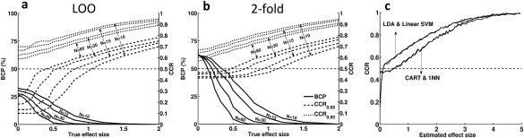
The effect of sample size, effect size, and classifier type on cross‐validated classification rates. (A) BCP, CCR_0.05, and CCR_0.95 as a function of true effect size and sample size for LDA with LOO cross‐validation. BCP is indicated on the left vertical axis, CCR_0.05 and CCR_0.95 on the right. (B) BCP, CCR_0.05, and CCR_0.95 as a function of true effect size and sample size for LDA with twofold cross‐validation. (C) Classification results for three parametric linear and two nonlinear classifiers using LOO cross‐validation. Linear classifiers show classification rates considerably below the chance level for small effect sizes, whereas the other two classifiers do not exhibit this phenomenon.

Figure 4a,b demonstrate the relationship of BCP, CCR_0.05, and CCR_0.95 with true effect size and sample size for LOO and twofold cross‐validation of LDA classification, respectively. In both cases, as either true effect size or sample size decreases, the probability of below chance classifications increases. In small samples, this value is already high for medium effect sizes [i.e. a mean difference of 0.7 standard deviation units following the conventions of Cohen, 1988]. Moreover, the “depth” of below chance classification rates as denoted by CCR_0.05 and the range of CCRs increases with decreasing true effect size or sample size. Thus, skewness and width of the distribution changes as a function of true effect size and sample size. Because of the asymmetry of the distribution (see Fig. 2d), some very low CCRs necessarily mean that there must be a larger number of moderately above chance results, even in the no effect case of $d=0$. Because the expected average CCR over all experiments with $d=0$ is 50%, each experiment with a CCR of 0% must be counterbalanced by 10 experiments with a CCR of 55%. This high number of positive results is obviously spurious and can be misleading if one is unaware of the skewness of the CCR distribution.

Comparison of Different Classifiers

Not all classifiers are susceptible to below chance classification rates (Fig. 4c). Only parametric linear classifiers (i.e. linear SVM and LDA) show expected values of their CCRs below the chance level when estimated effect sizes are low. The other two classifiers (Nearest Neighbor and CART), which do not depend on a linear metric, do not show average CCRs below chance level. The disadvantage of these nonlinear classifiers compared with the linear ones becomes obvious at larger effect sizes (here for $0.5<\widehat{d}<3$), where they have, on average, distinctly lower classification rates.

Classification Rate Versus Statistical Significance

Our results show that for twofold cross‐validation and small to medium effect sizes, more than 50% of experiments result in below chance level classification (Fig. 4a,b). On the other hand, CCRs for LOO can be much lower than for twofold cross‐validation. In the next set of experiments we look at whether a higher or a lower number of cross‐validation folds $k$ should be recommended for the use in hypothesis testing, in particular in LSS‐LES data. We studied the effect of $k$ on classification performance (CCR) and on its statistical significance. For this purpose, we generated synthetic data sets with the same procedure as before with $N=15$ observations per condition, which were drawn from two normally distributed populations. Population effect size varied from 0 to 1, estimated effect size was determined from the samples. The whole process was repeated 10,000 times for each set of parameters. Statistical significance was determined comparing the estimated CCR to a null distribution obtained from the 10,000 repetitions where population effect size was 0.

Figure 5a–d show the null distributions for twofold, fivefold, 10‐fold, and LOO cross‐validation, respectively. All cross‐validations were stratified except for LOO where only one trial was removed. Generally, increasing $k$ results in fewer, but more extreme below chance classifications. (LOO results in only 30.5% below chance classifications, twofold results in 62% BCP). In contrast, CCRs for LOO can reach 0%, whereas they remain above 40% for twofold. Because the expected values of these distributions, i.e. the mean CCRs over a large number of experiments, are fixed at 50%, most experiments using LOO cross‐validation must result in CCRs above 50%. From this consideration, it becomes clear that for $d=0$ LOO will result in more spuriously high CCRs than twofold cross‐validation.

Figure 5.

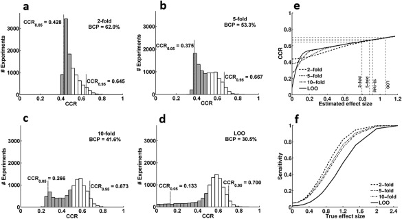
Effect of $k$ on CCRs of LDA with cross‐validation. (A–D) Null distributions for different values of $k$. Data come from 10,000 simulated experiments with a priori true effect size of $d=0$. They are classified with LDA using 2‐fold, 5‐fold, 10‐fold, and LOO cross‐validation, respectively. The gray areas show the experiments with classification rates below 50%. Because these distributions represent true effect sizes of $d=0$, mean CCRs are exactly 50%. (E) CCRs as a function of estimated effect size for various values of $k$. Estimated effect sizes and CCRs where significance is reached are indicated by dashed lines. (F) Sensitivity shows the ability of different cross‐validation procedures to correctly detect effects when true effect size is nonzero. For a given effect size $d$, the significance threshold of $P\le 0.05$ will be reached for smaller estimated effect sizes for twofold than for LOO cross‐validation and therefore, twofold shows higher sensitivity. For LOO, sensitivity can fall below 0.05 because its null‐distribution can only assume discrete values.

But, are the higher CCRs in LOO than in twofold cross‐validation a sign of a more sensitive test procedure in cases of $d>0$? Classification algorithms are typically optimized to reach high CCRs. This makes sense if classes are known to be distinct ( $d\gg 0$), and the focus is on correctly identifying novel items. For hypothesis testing purposes, however, the existence and size of a possible effect are unknown. Algorithms should therefore be optimized for highest sensitivity regarding the distinction between $d=0$ and $d>0$. Let us therefore assert that a reliable distinction is possible if a given CCR is higher than the CCR_0.95 of its null distribution. Figure 5e shows CCRs as a function of the estimated effect size $\widehat{d}$ for different values of $k$ (see also Appendix D for comparison in terms of AUC). For very large estimated effect sizes, the influence of $k$ can be neglected. For $0.1<\widehat{d}<1$, in this example, LOO shows higher CCRs than twofold cross‐validation. However, when testing for significance against the null distribution (Fig. 5a–d), the twofold procedure, although it needs on average larger effect sizes to attain the same CCR, reaches the threshold for significance (CCR_0.95) earlier than LOO (twofold: ${\widehat{d}}_{\mathrm{t}\mathrm{h}\mathrm{r}\mathrm{e}\mathrm{s}}=0.8$, LOO: ${\widehat{d}}_{\mathrm{t}\mathrm{h}\mathrm{r}\mathrm{e}\mathrm{s}}=1.1$). Together, LOO not only produces more spuriously high CCRs in the no effect case, it is also less sensitive than twofold cross‐validation when $\widehat{d}>0$. We can conclude that twofold cross‐validation should be preferred over LOO for hypothesis testing. CCRs should only be interpreted in relation to a suitable null distribution.

Generalization to High‐Dimensional Data

Finally, we studied how dimensionality of data affects classification performance. For this purpose, we analyzed the real EEG data set described above and compared it with synthetically generated data. We designed two series of 100 dimensional Monte Carlo experiments containing 30 observations per condition, which is comparable to the EEG data set. Simulations had a true effect size of zero to simulate the null distribution. In the first series, we assumed independent features; in the second series, features were correlated, as it is typically the case in neuroscience, e.g. in electrophysiological and imaging data. To obtain multivariate normal, correlated data, we generated 10,000 normally distributed, uncorrelated data sets, which were then multiplied by the Cholesky decomposition of a randomly generated covariance matrix. To derive the null distribution of our real EEG data, we used randomly shuffled class labels [Nichols and Holmes, 2002]. The three data sets were then classified with 3 popular linear classifiers, once using LOO and once using twofold cross‐validation.

Figure 6a shows the CCR distribution of real EEG data classified using LOO versus twofold (data for diagonal LDA, results for other classifiers are summarized in Table 1). CCRs for LOO are generally higher than for twofold, but in the below chance range LOO is also more extreme (CCR_min = 15%) than twofold (CCR_min = 39%). Despite the lower CCRs, twofold cross‐validation reaches significance sooner (59% in twofold vs. 63% in LOO) and shows higher sensitivity (13% of classifications significant with twofold, 9% of classifications significant with LOO). Looking at the null distribution obtained by shuffling EEG data labels shows that LOO and twofold procedures result in different distributions. LOO shows a strong skewness to the left giving CCRs as low as 0%, and a large number of spuriously high CCRs, with only 36.3% of classification rates below chance. twofold on the other hand shows a strong skewness to the right with a BCP of 59.6%. Together, these findings emphasize that twofold cross‐validation results less often in CCRs above 50%, but at the same time shows higher sensitivity than LOO cross‐validation (Fig. 6b–c).

Figure 6.

Searchlight classification of EEG data. (A) CCRs from LOO versus CCRs from a twofold procedure. Each dot represents the classification result of a single searchlight. Dashed lines indicate the average 5% significance threshold based on randomization tests. LOO results generally in higher CCRs, but twofold reaches significance for lower CCR values thus having a higher sensitivity. Percentages represent the proportion of tests that are below P < 0.05 for twofold and LOO, respectively. (B, C) Average null distribution of EEG searchlight classification obtained by random shuffling of class labels when classified using LOO and twofold. LOO results in more spuriously high CCRs, higher significance thresholds, and below chance classification rates close to 0%. Twofold produces more CCRs slightly below 50% under the null distribution and has a lower significance threshold and thus higher sensitivity.

Table 1.

BCP and range of null distribution for different classifiers based on real and synthetic EEG data when classified using LOO and twofold

	Real EEG data				Correlated data (synthetic)				Uncorrelated data (synthetic)
	Twofold		LOO		Twofold		LOO		Twofold		LOO
	BCP	Range	BCP	Range	BCP	Range	BCP	Range	BCP	Range	BCP	Range
NCC	59.1	43.4–59.6	36.4	26.7–63.3	62.0	44.7–60.2	28.5	16.7–65.0	50.4	41.3–58.9	49.5	33.3–65.0
DLDA	59.6	43.4–59.6	36.3	26.7–63.3	62.0	44.7–60.2	28.6	16.7–65.0	50.4	41.5–58.9	49.8	33.3–65.0
SVM	61.5	41.9–57.2	48.6	30.0–66.7	56.0	43.8–58.5	42.8	33.3–63.3	51.0	42.3–58.3	51.7	35.0–65.0

NCC: nearest centroid classifier, DLDA: diagonal LDA, SVM: support vector machine, BCP: below‐chance percentage, range: [CCR_0.05–CCR_0.95].

Comparing different linear classifiers (nearest centroid classifier [NCC], diagonal LDA, and linear SVM) shows that all of the linear classifiers tested here show asymmetric distributions for synthetic correlated data and real EEG data, i.e., higher than expected BCP for twofold, lower than expected BCP for LOO with asymmetric range (see Table 1). Both confirm the findings described in the previous sections.

Unlike correlated data, the null distributions of uncorrelated data show an almost symmetric structure, i.e. BCP of approximately 50% with nearly symmetric range. The effect of correlation can be understood by looking at multivariate effect sizes. In multidimensional data, the Mahalanobis distance $D=\sqrt{d^T{R}^{‐1}d}$ between two classes can be taken as the multivariate effect size. $d$ represents the vector of univariate effect sizes in each dimension, and $R$ is the correlation matrix of the data. When features are independent ( $R=I$), the Mahalanobis distance reduces to $\widehat{D}=\sqrt{{\widehat{d}}_1^2+{\widehat{d}}_2^2+\dots +{\widehat{d}}_p^2}$, with the empirical effects $\widehat{d}$ consisting of any true effect $d$ plus the measurement error $e$. Thus, the distance $\widehat{D}$ increases with increasing dimensionality even when no true effect is present at all. Therefore, inversions between training and test classification as described in Figure 3a become unlikely and less asymmetry in below chance classification rates occurs. A larger distance $\widehat{D}$ between conditions also allows the classifier to separate classes more easily, but, because no actual effect exists between conditions, this leads to overfitting the training data and no generalization to test data. Thus, CCRs for uncorrelated high‐dimensional data follow a symmetric distribution with BCP of 50%.

DISCUSSION

When we draw random samples from two normal distributions that do not differ in their means, the estimated differences of these means will be normally distributed around zero. When using MVPA on these data, one could assume that the distribution of classification rates is also distributed symmetrically around the chance level of 50%, following an approximately normal distribution. However, we show that our intuitive evaluation of results, based on assumptions of symmetry and normality, is misleading for classification outcomes. For classification with cross‐validation in typical life‐science data, i.e., small sample size data holding small effects, the distribution of classification rates is neither normal nor binomial [Noirhomme et al., 2014]. It can be strongly asymmetric and in some cases even bimodal. Its mode can lie either below or above the level expected by chance. Particularly for small effect sizes, we notice that the distribution of results can be strongly skewed and CCRs can sometimes fall far below chance level. Moreover, variance of CCR changes with effect size, disproportionally increasing for decreasing effect sizes and thus distorting CCR distribution further. This irregular distribution of CCRs implies that interpretation of CCRs as an indicator of presence or size of an effect is not advisable.

The aim of using MVPA for hypothesis testing is to detect the presence of differences between two or more conditions. CCR itself cannot be used for this purpose without a suitable critical value to compare it to. The level of this critical value can differ greatly depending on classifier, cross validation, number of features, sample size, and effect size in the data. Therefore, CCRs cannot be compared between different analyses in most cases. Instead, P values must be provided, which determine whether a certain CCR indicates a significant difference between classes. Significance testing always relies on an accurate estimation of the distribution of data under the null hypothesis. Importantly, the irregular shape of the CCR distribution forbids the use of parametric tests, which rely on normal or binomial null distributions. Instead, the null distribution should be established from surrogate data using Monte Carlo or randomization methods [Manly, 2007]. Furthermore, an maximization of CCR, which is perfectly reasonable when (infinite) novel stimuli must be identified, should never be done when cross‐validation is used in MVPA for hypothesis testing. This can be easily understood when looking at the comparison of twofold and LOO cross‐validation. Although the LOO procedure results in more above chance classifications, it is less sensitive, i.e., it requires a higher effect size to reach significance.

CCRs are unbiased, i.e. on average they are a good measure of classifiability. However, a problem occurs because of the skewness of the distribution, which shifts the mode of the distribution above or below its expected value. One particular danger when interpreting CCRs is that the presence of a few very strong below chance level CCRs must necessarily lead to a larger number of moderately above chance CCRs, even in data that do not contain any effect. This leads to several complications. First, although two methods (e.g. twofold and LOO) may have the same expected value for a certain true effect size, one will result in most cases in a higher CCR than the other (see Fig. 5). Any interpretation of this finding based on a small number of experiments will be misleading. Even if a large number of independent experiments is performed, the number of positive results will be similarly misleading. Only averaging CCRs over this larger number of experiments would generate a result close to the correct expected value. What is even worse, if those rare experiments or subjects resulting in very low CCRs are discarded as outliers or experimental failures and findings are not published, the average CCR of published studies will be clearly above 50%. Very few unpublished studies can then disproportionally distort conclusions of meta analyses. Similarly, if a number of identical analyses are carried out on a number of voxels, electrodes, genes, etc., the number of above 50% findings can be much higher than the number of below 50% findings although the null hypothesis is valid. If results (class differences, classifiability) are presented in terms of CCR, this can lead to the erroneous assumption that most dimensions (voxels, electrodes, or genes) carry class information. Any significance test that does not take the skewed distribution of CCRs into account has a high risk to result in a false positive finding.

Instead of using CCR to display classification results, we propose the use of P values for this purpose. While CCR behaves in a rather unintuitive fashion because of the skewness of its distribution when effect sizes are small, the distribution of P values is simple and most readers are familiar with their interpretation. This proposal follows the same logic that is used with fMRI analyses, which also usually present statistical maps rather than actual measures of hemodynamic responses. P values are a combined measure of central tendency, variability and sample size, and represent the strength of evidence against the null hypothesis. Given identical sample size, they provide a standardized way to compare results of different experiments, conditions and analyses. In addition, when using first and second level models, statistical values can be used to aggregate data over groups of subjects or compare data coming from different experimental conditions. If a suitable measure of multivariate effect size is available [see e.g. Allefeld and Haynes, 2014], then this should be presented and significances indicated. When no suitable measure of multivariate effect size is available, P values seem clearly preferable over CCRs to represent classification results.

The occurrence of classification rates far below the chance level in classification with cross‐validation has been observed in a number of studies before. It has been reported that LOO cross‐validation will in specific cases (e.g. linear SVM with a dimensionality approaching infinity) result in zero percent classification accuracy in finite data sets [Hall et al., 2005; Verleysen, 2003]. The same observation was reported for majority inducers irrespective of dimensionality [Kohavi, 1995]. We present analysis and simulations that help understand the causes underlying below chance classification. Occurrence of below chance classification is a direct result of the dependence of test and training means and thus in essence denotes that an effect is too small to be detected by the classifier. This strength of the dependence between training and test means depends on sample size and is also governed by $k$ in k‐fold cross validation.

The number of folds $k$ in cross‐validation affects the variance of classification accuracy and its significance, in particular, when sample size and estimated effect size are low. CCRs obtained by LOO are less likely to be below the chance level, but if they are, they are usually lower than for a twofold procedure. For medium estimated effect sizes LOO gives higher CCRs than twofold cross‐validation on average. This is desirable in a context of single item classification, when the presence of a class difference is known and the focus is on accurately classifying individual items. Previous studies therefore concluded that LOO should be preferred over twofold cross‐validation because of the latter's conservative bias [Kohavi, 1995; Rodriguez et al., 2010]. However, in a hypothesis testing context, when the presence of an effect is uncertain, twofold cross‐validation has a smaller variance, especially in the null‐distribution, and is therefore more reliable and reaches significance already with much smaller effect sizes than LOO. Using a twofold procedure is therefore preferable for hypothesis testing, because of its higher sensitivity, especially in LSS‐LES data.

Dimensionality of data is another important factor which affects the behavior of classification algorithms. Increasing the number of features impairs performance of classification algorithms, a fact also known as the “curse of dimensionality” [Bickel and Levina, 2004; Clarke et al., 2008; Fan and Fan, 2008]. Hall et al. showed that when the size of the feature vector increases with a fixed number of samples, linear SVM will asymptotically approach chance performance [Hall et al., 2005]. Jin et al. demonstrated that in data sets with few and weak relevant features classification can be impossible if feature selection is not done prior to classification [Donoho and Jin, 2008; Jin, 2009]. We showed in simulations and real EEG data that asymmetric distributions of CCRs with strong below chance classification rates and many spuriously high classification rates occur in high‐dimensional data as well as in low‐dimensional data, especially if features are correlated.

In this article, we have investigated the behavior of cross‐validation and MVPA in realistic life‐science data. This kind of data is often characterized by small effect sizes, small sample sizes, but a large number of features. We show that there are a few important guidelines that should be observed. Most importantly, the existence of an effect should not be determined by the classification rate, but rather by statistical significance, and significance should not be based on parametric tests, but on Monte Carlo methods. Furthermore, because hypothesis testing has different requirements than individual item identification, methods optimized for the latter purpose are not necessarily the best for the former. Therefore, although LOO cross‐validation results in higher classification rates, twofold cross‐validation is more suitable for hypothesis testing because its smaller variance makes it more sensitive. If these guidelines are observed, we believe that MVPA is an excellent method that allows dealing with the problems of multivariate data in the life‐sciences.

APPENDIX A. THEOREM 1

We assume a data set that consists of $N$ observations for each of two classes $A$ and $B$ with empirical means $\overrightarrow{m}={\left[m_A,m_B\right]}^T$. The means $m_{A,B}$ themselves are determined by the probability distributions $p_A\left(x_A\right)$ and $p_B\left(x_B\right)$ for the individual observations ${ x}_{A,B}$. We fix $m_A$ and $m_B$, thereby assuming the data set to be one specific realization of the random processes governed by $p_A$ and $p_B$. During k‐fold cross‐validation the data set is divided into a training and a test set, with means $\overrightarrow{\mu } ={[\mu }_A,{\mu }_B]$ for the training set and $\overrightarrow{\nu }={[\nu }_A,{\nu }_B]$ for the test set.

Under the definitions and assumptions above, the probability $\pi \left(\overrightarrow{m}\right)$ of a correct classification, conditional to the sample means $\overrightarrow{m}={\left[m_A,m_B\right]}^T$, is given by

$$\pi \left(\overrightarrow{m}\right)=\frac{1}{2}-\frac{1}{2}\left(\prod _{i=A,B}\int d{\mu }_i\mathrm{Pr}\left({\mu }_i|m_i\right)\right)({\varphi }_A-{\varphi }_B)\mathrm{s}\mathrm{i}\mathrm{g}\mathrm{n}({\mu }_A-{\mu }_B)$$

in which ${\varphi }_A$ is defined as ${\varphi }_A=:Pr\left(x_A\le \frac{{\mu }_A+ {\mu }_B}{2}|{\mu }_A<{\mu }_B,\overrightarrow{\mu },\overrightarrow{m}\right)$ and ${\varphi }_B$ is defined analogously.

Proof

For given sample means $m_{A,B}$, subsample means ${\mu }_{A,B}$ and ${\nu }_{A,B}$ are statistically dependent stochastic variables, since

$$m_{A,B}= \frac{{\mu }_{A,B}\left(k-1\right)+{\nu }_{A,B}}{k}$$ (1)

LDA in 1 − d is expressed by the two threshold conditions for correct classification of test observations $x_A$ and $x_B$ from the two classes

$$\left({\mu }_A- {\mu }_B\right)\left(x_A-t\right)\ge 0, \left({\mu }_A- {\mu }_B\right)\left(x_B-t\right)<0$$ (2)

Here, the discrimination threshold is the training mean:

$$t= \frac{{\mu }_A+ {\mu }_B}{2}$$ (3)

For given sample means $\overrightarrow{m} = {\left(m_A,m_B\right)}^T$ the probability ${\pi }_A$ of a correct classification of a test observation from class A ( $x_A$) is thus obtained as

$${\pi }_A\left(\overrightarrow{m}\right)=\int d\overrightarrow{\mu }[\mathrm{Pr}\left(x_A\ge t,{\mu }_A\ge {\mu }_B,\overrightarrow{\mu },\overrightarrow{m}\right)+\mathrm{P}\mathrm{r}(x_A\le t,{\mu }_A\le {\mu }_B,\overrightarrow{\mu },\overrightarrow{m})]$$ (4)

which can be further transformed as follows:

$${\pi }_A\left(\overrightarrow{m}\right)=\int d\overrightarrow{\mu }[\mathrm{Pr}\left(x_A\ge t|{\mu }_A\ge {\mu }_B,\overrightarrow{\mu },\overrightarrow{m}\right)\mathrm{Pr}\left({\mu }_A\ge {\mu }_B,\overrightarrow{\mu }|\overrightarrow{m}\right)+ \mathrm{Pr}\left(x_A\le t|{\mu }_A<{\mu }_B,\overrightarrow{\mu },\overrightarrow{m}\right)\mathrm{Pr}\left({\mu }_A<{\mu }_B,\overrightarrow{\mu }|\overrightarrow{m}\right)]$$ (5)

The two factors implementing the threshold connection are probabilities of complementary events and thus we can write:

$$\mathrm{Pr}\left(x_A\ge t|{\mu }_A\ge {\mu }_B,\overrightarrow{\mu },\overrightarrow{m}\right)=:1-{\varphi }_A$$ (6)

$$\mathrm{Pr}\left(x_A\le t|{\mu }_A<{\mu }_B,\overrightarrow{\mu },\overrightarrow{m}\right)=:{\varphi }_A$$ (7)

Using Eqs. (1) and (2), the probability ${\varphi }_A$ can be expressed as the cumulative distribution:

$${\varphi }_A=\underset{-\infty }{\overset{\frac{{\mu }_A+{\mu }_B}{2}}{\int }}d{x}_A\mathrm{Pr}\left(x_A|{\upsilon }_A\right)=\underset{-\infty }{\overset{\frac{{\mu }_A+{\mu }_B}{2}}{\int }}d{x}_A\frac{\mathrm{Pr}\left({\upsilon }_A|x_A\right)p_A\left(x_A\right)}{\mathrm{Pr}\left({\upsilon }_A\right)}=\underset{-\infty }{\overset{\frac{{\mu }_A+{\mu }_B}{2}}{\int }}d{x}_A\frac{\mathrm{Pr}\left(\sum _{\tau =1}^{T-1}{x}_A^{\tau }=T{\upsilon }_A-x_A\right)p_A\left(x_A\right)}{\mathrm{Pr}\left({\upsilon }_A\right)}$$ (8)

in which $T=N/k$ is the number of test observations.

The two remaining factors in Eq. (5) can again be evaluated using conditional probabilities:

$$\mathrm{Pr}\left({\mu }_A\ge {\mu }_B,\overrightarrow{\mu }|\overrightarrow{m}\right)=\mathrm{Pr}\left({\mu }_A\ge {\mu }_B|\overrightarrow{\mu },\overrightarrow{m}\right) \mathrm{Pr}\left(\overrightarrow{\mu }|\overrightarrow{m}\right)= \Theta \left({\mu }_A\ge {\mu }_B\right) \mathrm{P}\mathrm{r}\left({\mu }_A|m_A\right)\mathrm{P}\mathrm{r}\left({\mu }_B|m_B\right)$$ (9)

Here $\Theta$ denotes the Heavyside step function (indicator), and factorization of $\mathrm{Pr}\left(\overrightarrow{\mu }|\overrightarrow{m}\right)$ accounts for the independence of the classes.

In analogy, one obtains

$$\mathrm{Pr}\left({\mu }_A<{\mu }_B,\overrightarrow{\mu }|\overrightarrow{m}\right)=\Theta ({\mu }_A<{\mu }_B)\mathrm{P}\mathrm{r}\left({\mu }_A\right|m_A)\mathrm{P}\mathrm{r}({\mu }_B\left|m_B\right)$$ (10)

The probability ${\pi }_A$ of correct classification of a class A observation equals

$${\pi }_A\left(\overrightarrow{m}\right)=\left(\prod _{i=A,B}\int d{\mu }_i\mathrm{P}\mathrm{r}\left({\mu }_i\right|m_i)\right)[\left(1-{\varphi }_A\right)\Theta \left({\mu }_A\ge {\mu }_B\right)+{\varphi }_A\Theta \left({\mu }_A<{\mu }_B\right)]$$ (11)

Correspondingly, for class B:

$${\pi }_B\left(\overrightarrow{m}\right)=\left(\prod _{i=A,B}\int d{\mu }_i\mathrm{P}\mathrm{r}\left({\mu }_i\right|m_i)\right)[\left(1-{\varphi }_B\right)\Theta \left({\mu }_A<{\mu }_B\right)+{\varphi }_B\Theta \left({\mu }_A\ge {\mu }_B\right)]$$ (12)

Thus the probability of correct classification is

$$\pi \left(\overrightarrow{m}\right)= \frac{{\pi }_A\left(\overrightarrow{m}\right)+{\pi }_B\left(\overrightarrow{m}\right)}{2}=\frac{1}{2}-\frac{1}{2}\left(\prod _{i=A,B}\int d{\mu }_i\mathrm{Pr}\left({\mu }_i|m_i\right)\right)({\varphi }_A-{\varphi }_B)sign({\mu }_A-{\mu }_B)$$ (13)

Which completes the proof.

APPENDIX B. SIMPLIFICATION FOR NORMAL DISTRIBUTIONS

Example for the Case With No Effect

As an extreme example, we use Gaussian distributed data with no signal, i.e.

$$p_A\left(x\right)=p_B\left(x\right)=\mathcal{N}\left(x\right)=\frac{1}{\sqrt{2\pi }}\mathrm{e}\mathrm{x}\mathrm{p}\left(-\frac{x^2}{2}\right)$$ (14)

Applying Eq. (8) for the Gaussian distributions ${ p}_{A,B}$, the cumulative distribution is that of a Gaussian with variance $(T-1)/T$ and mean

$${\upsilon }_A=k{m}_A-(k-1){\mu }_A$$ (15)

This yields

$${\varphi }_A-{\varphi }_B=\mathrm{\Phi }\left(k\left({\mu }_A-m_A\right)+\frac{{\mu }_B-{\mu }_A}{2}\right)-\Phi \left(k\left({\mu }_B-m_B\right)+\frac{{\mu }_A-{\mu }_B}{2}\right)$$ (16)

with $\mathrm{\Phi }\left(z\right)=\frac{1}{2}[1 + \mathrm{e}\mathrm{r}\mathrm{f}(z/\sqrt{2(T-1)/T}\left)\right]$.

The conditional probabilities $\mathrm{P}\mathrm{r}\left({\mu }_i\right|m_i)$ are inferred from Bayes' law as

$$\mathrm{Pr}\left({\mu }_i|m_i\right)\propto \mathrm{Pr}\left(m_i|{\mu }_i\right)\mathrm{Pr}\left({\mu }_i\right)=\mathrm{Pr}\left[{\upsilon }_i=k{m}_i-\left(k-1\right){\mu }_i\right]\mathrm{P}\mathrm{r}\left({\mu }_i\right)$$ (17)

The means being sums of Gaussian variables, their distributions $\mathrm{P}\mathrm{r}\left({\mu }_i\right)$ and $\mathrm{P}\mathrm{r}\left({\upsilon }_i\right)$ are also Gaussians with variance $k/\left[\left(k-1\right)N\right]$ and $k/N$, respectively, and thus

$$\mathrm{Pr}\left({\mu }_i|m_i\right)=\sqrt{\frac{N(k-1)}{2\pi }}\mathrm{e}\mathrm{x}\mathrm{p}\left[\frac{N\left(k-1\right)}{2}{({\mu }_i-m_i)}^2\right]$$ (18)

Finally, we calculated the distributions of $\pi$ for $\overrightarrow{m}$ sampled from a Gaussian distribution

$$\mathrm{Pr}\left(m_i\right)=\sqrt{\frac{N}{2\pi }}\mathrm{e}\mathrm{x}\mathrm{p}\left[-m_i^2(N/2)\right]$$ (19)

Example for the Case With an Effect of $\mathit{d}>0$

The previous Gaussian example can be easily generalized to finite signal strength $d$ by letting

$$p_A\left(x\right)={\mathcal{N}\left(x+\frac{d}{2}\right), p}_B\left(x\right)=\mathcal{N}\left(x-\frac{d}{2}\right)$$ (20)

In this case both the difference ${\varphi }_A-{\varphi }_B$ from Eq. (16) and $\mathrm{Pr}\left({\mu }_i|m_i\right)$ from Eq. (18) are unchanged, since they only depend on differences of means. Thus Eq. (13) for $\pi \left(\overrightarrow{m}\right)$ still holds in this case. The only difference between the case with and without effect therefore derives from the sampling of $\overrightarrow{ m}$. As a result of $d\ne 0$ the part of the function $\pi \left(\overrightarrow{m}\right)$ that is sampled is further away from the valley of below‐chance classification rates and therefore the distribution of $\pi$ is less skewed than in the no effect case.

To validate our analytical results, we generated a series of simulations with different effect sizes and calculated CCRs once using k‐fold cross‐validation and once with Eq. (13). As Figure B1 shows, the results are fairly similar.

APPENDIX C. COROLLARY 1

Corollary 1

The probability of correct classification in LDA with cross‐validation for no effect data sets ( $m_A=m_B$) must always be below the level expected for chance classification. This result is independent of the data distribution and the number of cross‐validation folds $k$.

Proof

From Theorem 1 we know:

$$\pi \left(\overrightarrow{m}\right)=\hspace{0.17em}\frac{{\pi }_A\left(\overrightarrow{m}\right)+{\pi }_B\left(\overrightarrow{m}\right)}{2}=\frac{1}{2}-\frac{1}{2}\left(\prod _{i=A,B}\int d{\mu }_i\mathrm{Pr}\left({\mu }_i|m_i\right)\right)\left({\varphi }_A-{\varphi }_B\right)sign\left({\mu }_A-{\mu }_B\right)$$ (21)

The integral on the right side represents the deviation from chance level, i.e., 0.5. Here we show that for data with an estimated effect size of zero, the integrand will be always positive thus leading to below chance values of $\pi \left(\overrightarrow{m}\right)$. To prove this it suffices to show that $\left({\varphi }_A-{\varphi }_B\right)\mathrm{s}\mathrm{i}\mathrm{g}\mathrm{n}\left({\mu }_A-{\mu }_B\right)>0$ because $\mathrm{Pr}\left({\mu }_i|m_i\right)>0$ by definition.

According to Eq. (8), for $m=m_A=m_B$ we can write

$${\varphi }_A-{\varphi }_B=\int dx\left[\mathrm{P}\mathrm{r}\left(x|km-\left(k-1\right){\mathrm{\mu }}_A\right)-\mathrm{P}\mathrm{r}\left(x|km-\left(k-1\right){\mathrm{\mu }}_B\right)\right].$$

If ${\mu }_A>{\mu }_{B, }$ the left summand under the integral is a left‐shifted version of the right summand. Since being probabilities, both summands are positive and normalized, the difference ${\varphi }_A-{\varphi }_B$ is positive. Conversely, for ${\mu }_A<{\mu }_B$ the difference ${\varphi }_A-{\varphi }_B$ is negative. Thus, in both cases $\left({\varphi }_A-{\varphi }_B\right)sign\left({\mu }_A-{\mu }_B\right)>0$ and the corollary is proved.

APPENDIX D. AREA UNDER THE CURVE (AUC)

AUC is similarly affected by the dependence of the sub‐sample means. Using classification thresholds as it is done in AUC does not prohibit negative correlations between test and training means. Figure D1 replicates Figure 5e for AUC.

Figure B1.

Cumulative distribution function of CCRs for LDA ( $N=15$) using different values of $k$ calculated from Eq. (13) (gray lines) and determined using simulation results (black lines). The results show that both Eq. (13) and simulations produce very similar results.

Figure D1.

The dependence of the subsample means affects performance of an LDA classifier largely independently of performance measure. Using a signal detection approach and replacing CCR with the area under the curve (AUC) from receiver operating characteristics (ROC) curves results in AUCs below 0.5.

REFERENCES

- Allefeld C, Haynes JD (2014): Searchlight‐based multi‐voxel pattern analysis of fMRI by cross‐validated MANOVA. Neuroimage 89:345–357. [DOI] [PubMed] [Google Scholar]
- Azuaje F (2003): Genomic data sampling and its effect on classification performance assessment. BMC Bioinf 4:5. [DOI] [PMC free article] [PubMed] [Google Scholar]
- Bickel PJ, Levina E (2004): Some theory for Fisher's linear discriminant function, 'naive Bayes', and some alternatives when there are many more variables than observations. Bernoulli 10:989–1010. [Google Scholar]
- Braga‐Neto UM, Dougherty ER (2004): Is cross‐validation valid for small‐sample microarray classification? Bioinformatics (Oxford, England) 20:374–380. [DOI] [PubMed] [Google Scholar]
- Button KS, Ioannidis JP, Mokrysz C, Nosek BA, Flint J, Robinson ES, Munafo MR (2013): Power failure: Why small sample size undermines the reliability of neuroscience. Nat Rev Neurosci 14:365–376. [DOI] [PubMed] [Google Scholar]
- Clarke R, Ressom HW, Wang A, Xuan J, Liu MC, Gehan EA, Wang Y (2008): The properties of high‐dimensional data spaces: implications for exploring gene and protein expression data. Nat Rev Cancer 8:37–49. [DOI] [PMC free article] [PubMed] [Google Scholar]
- Cohen J (1988): Statistical Power Analysis for the Behavioral‐Sciences. NJ: Lawrence Erlbaum Associates. [Google Scholar]
- Damarla SR, Just MA (2013): Decoding the representation of numerical values from brain activation patterns. Hum Brain Mapp 34:2624. [DOI] [PMC free article] [PubMed] [Google Scholar]
- Delorme A, Makeig S (2004): EEGLAB: an open source toolbox for analysis of single‐trial EEG dynamics including independent component analysis. J Neurosci Methods 134:9–21. [DOI] [PubMed] [Google Scholar]
- Deuker L, Olligs J, Fell J, Kranz TA, Mormann F, Montag C, Reuter M, Elger CE, Axmacher N (2013): Memory consolidation by replay of stimulus‐specific neural activity. J Neurosci 33:19373–19383. [DOI] [PMC free article] [PubMed] [Google Scholar]
- Donoho D, Jin JS (2008): Higher criticism thresholding: Optimal feature selection when useful features are rare and weak. Proc Natl Acad Sci USA 105:14790–14795. [DOI] [PMC free article] [PubMed] [Google Scholar]
- Dougherty ER (2001): Small sample issues for microarray‐based classification. Comp Funct Genomics 2:28–34. [DOI] [PMC free article] [PubMed] [Google Scholar]
- Duarte JV, Ribeiro MJ, Violante IR, Cunha G, Silva E, Castelo‐Branco M (2014): Multivariate pattern analysis reveals subtle brain anomalies relevant to the cognitive phenotype in neurofibromatosis type 1. Hum Brain Mapp 35:89–106. [DOI] [PMC free article] [PubMed] [Google Scholar]
- Etzel JA, Zacks JM, Braver TS (2013): Searchlight analysis: Promise, pitfalls, and potential. Neuroimage 78:261–269. [DOI] [PMC free article] [PubMed] [Google Scholar]
- Fan JQ, Fan YY (2008): High dimensional classification using features annealed independence rules. Ann Stat 36:2605–2637. [DOI] [PMC free article] [PubMed] [Google Scholar]
- Fuentemilla L, Penny WD, Cashdollar N, Bunzeck N, Duzel E (2010): Theta‐coupled periodic replay in working memory. Curr Biol 20:606–612. [DOI] [PMC free article] [PubMed] [Google Scholar]
- Gisselbrecht SS, Barrera LA, Porsch M, Aboukhalil A, Estep PW3, Vedenko A, Palagi A, Kim Y, Zhu X, Busser BW, Gamble CE, Iagovitina A, Singhania A, Michelson AM, Bulyk ML (2013): Highly parallel assays of tissue‐specific enhancers in whole Drosophila embryos. Nat Methods 10:774–780. [DOI] [PMC free article] [PubMed] [Google Scholar]
- Hall P, Marron JS, Neeman A (2005): Geometric representation of high dimension, low sample size data. J R Stat Soc Ser B Stat Methodol 67:427–444. [Google Scholar]
- Hastie T, Tibshirani R, Friedman J (2001): The Elements of Statistical Learning. New York: Springer. [Google Scholar]
- Haynes JD, Rees G (2006): Decoding mental states from brain activity in humans. Nat Rev Neurosci 7:523–534. [DOI] [PubMed] [Google Scholar]
- Jin JS (2009): Impossibility of successful classification when useful features are rare and weak. Proc Natl Acad Sci USA 106:8859–8864. [DOI] [PMC free article] [PubMed] [Google Scholar]
- Kamitani Y, Tong F (2005): Decoding the visual and subjective contents of the human brain. Nat Neurosci 8:679–685. [DOI] [PMC free article] [PubMed] [Google Scholar]
- Kohavi, R. (1995) A study of cross‐validation and bootstrap for accuracy estimation and model selection. In: Proceedings of the 14th international joint conference on Artificial intelligence, Vol. 2. Montreal, Quebec, Canada: Morgan Kaufmann Publishers Inc. pp 1137–1143.
- Kriegeskorte N, Goebel R, Bandettini P (2006): Information‐based functional brain mapping. Proc Natl Acad Sci USA 103:3863–3868. [DOI] [PMC free article] [PubMed] [Google Scholar]
- Kriegeskorte N, Simmons WK, Bellgowan PS, Baker CI (2009): Circular analysis in systems neuroscience: The dangers of double dipping. Nat Neurosci 12:535–540. [DOI] [PMC free article] [PubMed] [Google Scholar]
- Lemm S, Blankertz B, Dickhaus T, Muller KR (2011): Introduction to machine learning for brain imaging. Neuroimage 56:387–399. [DOI] [PubMed] [Google Scholar]
- Manly BFJ (2007): Randomization, Bootstrap, and Monte Carlo Methods in Biology. Boca Raton, FL: Chapman & Hall/CRC. [Google Scholar]
- Nichols TE, Holmes AP (2002): Nonparametric permutation tests for functional neuroimaging: A primer with examples. Hum Brain Mapp 15:1–25. [DOI] [PMC free article] [PubMed] [Google Scholar]
- Noirhomme Q, Lesenfants D, Gomez F, Soddu A, Schrouff J, Garraux G, Luxen A, Phillips C, Laureys S (2014): Biased binomial assessment of cross‐validated estimation of classification accuracies illustrated in diagnosis predictions. Neuroimage Clin 4:687–694. [DOI] [PMC free article] [PubMed] [Google Scholar]
- Norman KA, Polyn SM, Detre GJ, Haxby JV (2006): Beyond mind‐reading: Multi‐voxel pattern analysis of fMRI data. Trends Cognit Sci 10:424–430. [DOI] [PubMed] [Google Scholar]
- Raudys S, Pikelis V (1980): On dimensionality, sample size, classification error, and complexity of classification algorithm in pattern recognition. IEEE Trans Pattern Anal Mach Intell 2:242–252. [DOI] [PubMed] [Google Scholar]
- Raudys SJ, Jain AK (1991): Small sample size effects in statistical pattern recognition: Recommendations for practitioners. IEEE Trans Pattern Anal Mach Intell 13:252–264. [Google Scholar]
- Rodriguez JD, Perez A, Lozano JA (2010): Sensitivity analysis of k‐fold cross validation in prediction error estimation. IEEE Trans Pattern Anal Mach Intell 32:569–575. [DOI] [PubMed] [Google Scholar]
- Staresina BP, Alink A, Kriegeskorte N, Henson RN (2013): Awake reactivation predicts memory in humans. Proc Natl Acad Sci USA 110:21159–21164. [DOI] [PMC free article] [PubMed] [Google Scholar]
- Verleysen M (2003): Learning high‐dimensional data. Limit Future Trends Neural Comput 2. pp 141–162. [Google Scholar]