Resting‐state networks in 6‐to‐10 year old children

Abstract

Resting‐state functional magnetic resonance imaging provides a non‐invasive approach to the study of intrinsic functional brain networks. When applied to the study of brain development, most studies consist of relatively small samples that are not always representative of the general population. Descriptions of these networks in the general population offer important insight for clinical studies examining, for instance, psychopathology or neurological conditions. Thus our goal was to characterize resting‐state networks in a large sample of children using independent component analysis (ICA). The study further aimed to describe the robustness of these networks by examining which networks occur frequently after repeated ICA. Resting‐state networks were obtained from a sample of 536 6‐to‐10 year old children. Distributions of networks were built from repeated subsampling and group ICA analyses, and meta‐ICA was used to construct a representative set of components. Within‐ and between‐network properties were tested for age‐related developmental associations using spatio‐temporal regression. After repeated ICA, many networks were present over 95% of the time suggesting the components are highly reproducible. Some networks were less robust, and were observed less than 70% of the time. Age‐related associations were also observed in a selection of networks, including the default‐mode network, offering further evidence of development in these networks at an early age. ICA‐derived resting‐state networks appear to be robust, although some networks should further scrutinized if subjected to group‐level statistical analyses, such as spatiotemporal regression. The final set of ICA‐derived networks and an age‐appropriate T₁‐weighted template are made available to the neuroimaging community, https://www.nitrc.org/projects/genr. Hum Brain Mapp 37:4286–4300, 2016. © 2016 Wiley Periodicals, Inc.

INTRODUCTION

Resting‐state functional magnetic resonance imaging (RS‐FMRI) relies on a phenomenon referred to as intrinsic brain activity, or brain activity that is not induced by an external stimulus. In the context of RS‐FMRI, functional connectivity is explored when temporal fluctuations in blood oxygen level‐dependent maps are used to identify brain regions with high temporal correlation. Quantifying functional connectivity can be achieved through various analysis strategies, such as seed‐based analyses, graph theoretical models, and independent component analyses (ICA) [Cole, et al., 2010]. The ICA of RS‐FMRI data aims to reduce complex data into statistically distinct components [Beckmann et al., 2005; Calhoun et al., 2001]. These distinct components can be classified to describe either brain RS‐FMRI networks (RSNs, e.g., the default mode network) or noise signals (e.g., motion, flow artifact, non‐neuronal physiological noise). However, heterogeneity exists in the literature in terms of the selection (subset) of components reported; for instance, one study of children reports the executive control network [Jolles et al., 2011] while another does not [de Bie et al., 2012]. Further, reports of RSNs from ICA are limited in young children and are typically based on relatively small sample sizes.

Studying RSNs in healthy children contributes significantly to the literature, both in terms of describing normal brain development and in comparisons with neurological and psychiatric problems. To date, three studies have used a pure ICA approach to examine RSNs in young, typically developing children [de Bie et al., 2012; Jolles et al., 2011; Littow et al., 2010]. In a study of 5‐to‐8 year old children (n = 18), de Bie et al. [2012] labeled fourteen components as RSNs, based on the anatomical locations of the spatial maps, and the power spectra of the accompanying time series. Jolles et al. [2011] examined a sample of 11‐to‐13 year olds (n = 19) and a group of young adults (n = 29) using RS‐FMRI. Thirteen components were labeled as functionally relevant and were further evaluated for age‐related differences. Finally, Littow et al. [2010] examined a large sample (n = 168) of healthy adolescents and adults, categorized into three groups: adolescents, young adults, and older adults. The authors identified 21 RSNs, some of which showed differences across the age‐groupings, both in terms of spatial extent of the components and the power spectra. In addition to the to the above literature in children and adolescents, certain resting‐state components, including the default mode network, have also been identified very early in development [Gao et al., 2009].

In both the adult and pediatric literature, two specific aspects of ICA analysis deserve mention. First, many common ICA algorithms available for use with RS‐FMRI data operate under certain assumptions to increase efficiency, given the computational resources necessary to accommodate the magnitude of information in typical FMRI datasets. This has been shown to lead to variability in the resulting components [Franco et al., 2013; Himberg et al., 2004]. Along similar lines, other unexpected factors that are algorithm‐dependent can influence components resulting from ICA, such as subject order [Zhang et al., 2010]. Secondly, in many studies utilizing group ICA, only the components of interest are commonly reported, meaning components of non‐interest or noise are often neglected. Thus, there is variability in the literature in terms of the components that are examined, which may be related to methodological aspects of ICA analysis, or simply because of subjectivity in which components are reported. Further, it is possible that some of these ‘noise’ components, such as those related to susceptibility artifact or to blood flow artifact, will be highly consistent across studies, while others (e.g., thermal or scanner‐specific) will not. The presence or absence of certain components may also be impacted by the level of “cleaning” or “denoising” applied to the data, for instance censoring corrupt volumes [Power et al., 2012] or ICA‐based artifact removal [Griffanti et al., 2014]. This is of particular importance when studying children, given their tendency to have higher levels of motion compared to adults [Satterthwaite et al., 2012].

Within this context, it was the goal of this study to characterize ICA‐derived resting‐state networks in school‐age children. We utilized a large sample of 6‐to‐10 year old children to develop an age‐appropriate, standardized set of RSNs using a subsampling approach to account for some of the sources of variability. We hypothesized some networks (for instance those reported frequently in the literature) would be robust across multiple ICA analyses, whereas others would be observed less frequently. We also examine developmental aspects in a subset of components by using within‐ and between‐network age‐associations. The present study expands upon the current literature in multiple ways. First, the only other resting‐state studies in children utilizing ICA are based on relatively small samples. Second, RS‐FMRI studies utilizing ICA typically report only a subset of the components identified, making more global comparisons across studies difficult. Lastly, the current study reports on the frequency different components are identified by ICA, offering future work a framework for deciding what level of caution to be used when interpreting results from certain low‐frequency components. Components robust against repeated subsampling can be regarded as valid in previous studies and confidently analyzed in future efforts. Components shown to be more variable should be interpreted carefully, as they could be the result of a number of factors, including age‐related effects, individual differences, or even artifacts or methodological issues.

MATERIALS AND METHODS

Participants

The current study is embedded in the Generation R Study, which is a large, population‐based birth cohort in Rotterdam, the Netherlands [Jaddoe et al., 2012]. One thousand seventy children, ages 6‐to‐10 years, were scanned between September 2009 and July 2013 as part of a sub‐study within the Generation R Study [White et al., 2013]. General exclusion criteria for the current study include severe motor or sensory disorders (deafness or blindness), neurological disorders, moderate to severe head injuries with loss of consciousness, claustrophobia, and contraindications to MRI. Informed consent was obtained from parents, and all procedures were approved by the Medical Ethics Committee of the Erasmus Medical Center.

Of the 1,070 children with an MR‐scanning session, 964 completed a RS‐FMRI scan. Of the children with a RS‐FMRI scan, 652 were characterized as not having behavioral problems (see section “Behavioral assessment” below for assessment of child behavioral problems). Of those 652 data sets, 88 showed excessive motion (described in section “Data quality”), and an additional 28 datasets had problems with pre‐processing (e.g., poor registration to common space) rendering them unfit for post‐processing. Thus, 536 children (mean age 7.9 years, 49% female) were included in the final sample for data analysis (Table 1).

Table 1.

Sample characteristics

	N = 536
Child characteristics
General
Age at MRI (years)	7.96 ± 0.98
Sex (M/F, %)	51.5/48.5
Non‐verbal IQ	103.8 ± 14.0
Handedness (right/left, %)	89.9/10.1
Ethnicity
Dutch (%)	75.9
Non‐Western (%)	16.6
Other Western (%)	7.5
FMRI motion parameters
Avg. RMS relative (mm)	0.13 ± 0.11
Maternal characteristics
Educational level (%)
Primary	5.0
Secondary	40.3
Higher	54.6

Note: Data presented are mean ± standard deviation, unless otherwise noted.

Behavioral Assessment

Behavioral problems in children were assessed through maternal report using the Child Behavioral Checklist (CBCL/1½‐5) [Achenbach and Rescorla, 2000] as part of the age 6 assessment wave [Tiemeier et al., 2012]. The CBCL is a 99‐item inventory that uses a Likert response format (e.g., “Not True,” “Somewhat True,” “Very True”). Seven syndrome scales, five DSM‐oriented scales, and three broadband scales are commonly derived summary measures from the CBCL [Achenbach and Ruffle, 2000; Tick et al., 2007]. In order to obtain a set of networks that are not influenced by potentially aberrant networks that may be present in children with behavioral problems, participants who scored higher than the clinical cutoff on any syndrome scale, DSM‐oriented scale, broadband scale, or total problems score were excluded from analyses. Cutoff scores used in this study were based on norms from the Dutch population [Tick et al., 2007]. As mentioned above, of the 964 children with an RS‐FMRI scan, 312 children with CBCL scores above the clinical cutoff were excluded.

MR Data Acquisition

Magnetic resonance imaging data were acquired on a 3 Tesla scanner (Discovery 750, General Electric, Milwaukee, WI) using a standard 8‐channel, receive‐only head coil. A three‐plane localizer was run first and used to position all subsequent scans. Structural T₁‐weighted images were acquired using a fast spoiled gradient‐recalled echo (FSPGR) sequence [TR = 10.3 ms, TE = 4.2 ms, TI = 350 ms, NEX = 1, flip angle = 16°, matrix = 256 × 256, field of view (FOV) = 230.4 mm, slice thickness = 0.9 mm]. Echo planar imaging was used for the RS‐FMRI session with the following parameters: TR = 2,000 ms, TE = 30 ms, flip angle = 85°, matrix = 64 × 64, FOV = 230 mm × 230 mm, slice thickness = 4 mm. In order to determine the number of TRs necessary for functional connectivity analyses, early acquisitions acquired 250 TRs (acquisition time = 8 min 20 sec). After it was determined fewer TRs were required for these analyses, the number of TRs was reduced to 160 (acquisition time = 5 min 20 sec, see section “MR data pre‐processing” for additional details) [Langeslag et al., 2012; White et al., 2014]. Children were instructed to stay awake, keep their eyes closed, and not to think about anything in particular during the RS‐FMRI scan. Further details on the entire scanning protocol can be found elsewhere [White et al., 2013].

MR Data Processing

MR data pre‐processing

Data were first converted from DICOM to Nifti format using the “dcm2nii” tool from the MRIcro library (http://www.mccauslandcenter.sc.edu/mricro/mricron/dcm2nii.html). Prior to analysis, in cases where 250 RS‐FMRI volumes were acquired (see section “MR data acquisition”), the scans were trimmed to 160 volumes by omitting volumes at the end of the acquisition to ensure full compatibility with the other, 160 volume datasets. Data were pre‐processed using the Functional MRI of the Brain (FMRIB) Software Library (v5.0.5, FSL, http://fsl.fmrib.ox.ac.uk/fsl/fslwiki) [Jenkinson et al., 2012]. FSL's FMRI Expert Analysis Tool (FEAT) was used for preprocessing the RSFMRI data, which consisted of exclusion of the first four volumes, motion correction, high‐pass temporal filtering (sigma = 50), brain extraction, and spatial filtering (FWHM = 8 mm). Registration of the RS‐FMRI data to an age‐appropriate, standard space, T₁‐weighted template (see section “Study‐specific, age‐appropriate template for registration” for details) was achieved using a two‐step process. First, the RS‐FMRI data were registered to the T₁‐weighted anatomical image with the FSL‐Linear Registration Tool (FLIRT), using 6 degrees of freedom (DOF) and the boundary based registration (BBR) cost function. In the second stage, the T₁‐weighted image was registered to the age‐appropriate, standard space T₁‐weighted template image using FLIRT with 12 DOF. The two resulting transformation matrices were concatenated and applied to the preprocessed RS‐FMRI data.

Subject‐level ICA‐based artifact removal

In addition to standard FMRI pre‐processing, each data set was cleaned to remove potential biases resulting from subject motion, cardiac/respiratory physiology, and scanner noise using the FMRIB ICA‐based Xnoiseifier [FIX v1.06, Griffanti et al., 2014; Salimi‐Khorshidi et al., 2014]. With the aid of a training set, FIX automatically classifies subject‐level ICA components as “signal” or “noise,” and subsequently “denoises” the RS‐FMRI data by regressing out time series classified as noise. A thorough and sophisticated cleaning procedure, such as FIX, is especially relevant in the context of pediatric RS‐FMRI, given recent reports on the impact of motion on functional connectivity [Power et al., 2012; Satterthwaite et al., 2012]. All RS‐FMRI datasets underwent a single‐session ICA using the Multivariate Exploratory Linear Optimized Decomposition into Independent Components (MELODIC, v5.0.5) tool from FSL, followed by the artifact removal with FIX, including the removal of motion confounds [Griffanti et al., 2014]. The FIX classifier was trained using manually labeled, subject‐level ICA data from a random sample of 50 subjects with usable data. Briefly, the subject‐level ICA data from these 50 subjects was loaded into the Melview viewer (http://fsl.fmrib.ox.ac.uk/fsl/fslwiki/Melview), and both the spatial and temporal (power spectrum and time series) characteristics were used to classify components as either “signal” or “noise.” The performance of the training set was then measured using a leave‐one‐out cross validation, where a single subject is excluded from the training set, which is subsequently used to classify that (left out) subject's data. We found the training set to perform well, with a mean true‐positive rate (correctly labeled “signal” components) of 93.4% and a true negative rate (correctly labeled “noise” components) of 85.8%.

Study‐specific, age‐appropriate template for registration

Given the age of the sample, it was important to use an age‐appropriate template for registration of the functional data to standard space. One hundred thirty T₁‐weighted images from children without behavioral problems, also rated as having excellent quality, were used to construct the structural template for registration. An iterative approach using both linear and nonlinear algorithms was used [Sanchez et al., 2012], and is represented graphically in the supplemental data section (Supporting Information Fig. I). Briefly, T₁‐weighted images from each of the 130 subjects were first aligned to the MNI‐152 1mm brain using a linear, 6 degree of freedom approach (FLIRT). All registered images were then averaged and used as the template brain for the subsequent step, which was a nonlinear registration (FNIRT). Once again, the result from the nonlinear registration was averaged and used as the template for the subsequent iteration. This routine continued for a total of five nonlinear iterations, where it has been shown the template image stabilizes considerably [Sanchez et al., 2012]. The result of the fifth and final nonlinear registration was averaged, resampled to 2 mm isotropic resolution, and then used as the standard‐space template for all RS‐FMRI datasets. The average age and IQ, and the distribution of sex and handedness of the subjects used in creating the template was similar to that of the larger sample used in RS‐FMRI analyses (age = 7.86 ± 0.99, IQ = 105 ± 14.0, sex = 50.4% Female, 49.6% Male, handedness = 90.2% Right, 9.8% Left).

Data quality

Data quality was assessed in two steps. First, as the subject‐level ICA de‐noising of the data is not sufficient in datasets severely corrupted by motion, a mean root‐mean‐squared relative motion greater than 0.5 mm was used as a cutoff to exclude data of poor quality (n = 88). Second, all standard space registrations were examined using the middle functional volume from the time‐series, and poorly registered datasets were excluded (n = 28). Registrations were checked by merging the middle, three‐dimensional (3D) functional volume from each participant into a single four‐dimensional (4D) nifti file, and scrolling through the images, inspecting for gross translational or rotational shifts from the standard‐space template (>1 voxel shift).

Independent component analyses

Two ICA approaches were utilized. For the first approach, a repeated subsampling was used to generate distributions of the functional connectivity components and identify which were robust across multiple ICA runs. In total, 500 resamples were completed. For a given resample, 50 datasets were randomly selected from the pool of 536 datasets, and run through the multisession temporal concatenation method from the MELODIC tool from FSL (v5.0.5) to generate spatial component maps. Dimensionality was set to 25 components, as a large number of previous studies used a similar value and our tests with these data showed robust networks that correspond with existing reports in the literature [de Bie et al., 2012; Jolles et al., 2011; Smith et al., 2009]. The decision to use 50 cases per resample was guided by current, typical sample sizes in RS‐FMRI studies. For the second approach, the components resulting from the 500 resamples (25 components × 500 subsamples = 12,500 components) were summarized using a meta‐ICA [Biswal et al., 2010], with the dimensionality set to 25 to match that of the individual group ICA runs. Components resulting from the meta‐ICA were further summarized anatomically by determining overlap with the Harvard–Oxford anatomical atlases available in FSL after being registered to the MNI152 brain using a linear transform [Desikan et al., 2006].

Within‐ and between‐network associations

In order to explore age‐related associations with various ICA‐derived networks, the “Dual Regression,” or spatiotemporal regression, approach from FSL was utilized to generate subject‐specific time courses and spatial maps for each component [Filippini et al., 2009]. In the first step of the Dual Regression, the spatial components resulting from the above‐described meta ICA were regressed on each subject's denoised RS‐FMRI data to create subject‐specific time courses for each component. Next, these time courses were regressed on the RS‐FMRI data to create subject‐specific spatial maps for each component.

To study within‐network associations and limit the number of tests performed, four networks of interest were selected (right and left parietofrontal networks, default mode network, and executive control network) and whole‐brain, voxel‐wise statistics were employed on the dual regression maps using the FSL tool “Randomise” [Winkler et al., 2014]. The General Linear Model was used, with age entered as the predictor of interest and sex, ethnicity (dummy‐coded with Dutch as the reference), and total CBCL behavioral problems entered as covariates. For each contrast, 10,000 permutations were run, and the threshold‐free cluster enhancement option was utilized [Smith and Nichols, 2009]. To account for the number of voxel‐wise statistical tests run, P‐values were adjusted for Family‐wise error (FWE). Further, given that four networks were examined, a simple Bonferroni correction was applied to FWE‐corrected p‐value maps to indicate significance (where P _corrected < 0.05 from this point on is based on Bonferroni correction due to the four networks, positive and negative age contrasts, yielding eight tests and P < 0.00625 applied to FWE corrected maps).

Between‐network associations were studied with the Matlab‐based (vR2011B, Mathworks Inc., Natick, MA) “FSLnets” plugin (http://fsl.fmrib.ox.ac.uk/fsl/fslwiki/FSLNets). A 13 × 13 correlation matrix of non‐noise networks was built by correlating subject‐specific time courses from the dual regression analysis for each component of interest, after regressing away components labeled as noise. Correlation coefficients were then transformed to z‐values, and were subsequently used in statistical analyses with the randomise tool. As above in within‐network analyses, randomise was used to associate age with each cell in the lower half of the correlation matrix, with sex, ethinicity, and total CBCL behavioral problems entered as covariates. Using data from 10,000 permutations, correction for multiple testing was again attained with FWE correction.

RESULTS

Meta ICA

The spatial components from the 500 subsamples were summarized using a meta‐ICA and the results are depicted in Figures 1, 2, 3. Numerous components previously described in adults were observed, including the default‐mode, lateralized frontoparietal, parietal, sensorimotor, visual networks [Damoiseaux et al., 2006; Smith et al., 2009]. In addition to true RSNs, networks likely resulting from noise (physiological, scanner, image processing, etc.) are also depicted. Table 2 outlines basic anatomical information about the components and also includes the ratio of summed power above/below 0.1 Hz, averaged across the 500 subsamples, for each component. This power ratio has been indicated in previous work as a useful metric in classifying components as true RSNs and noise. Intrinsic functional connectivity is thought to be most represented in the 0.01–0.10 Hz range, and noise resulting from various sources is represented at higher frequencies. For instance, components 6 and 7, both in the brainstem, have a high‐to‐low power ratio 2‐to‐3 times that of true RSNs, such as the default‐mode and frontoparietal networks, indicating the majority of the represented frequencies are above the 0.10 Hz level.

Figure 1.

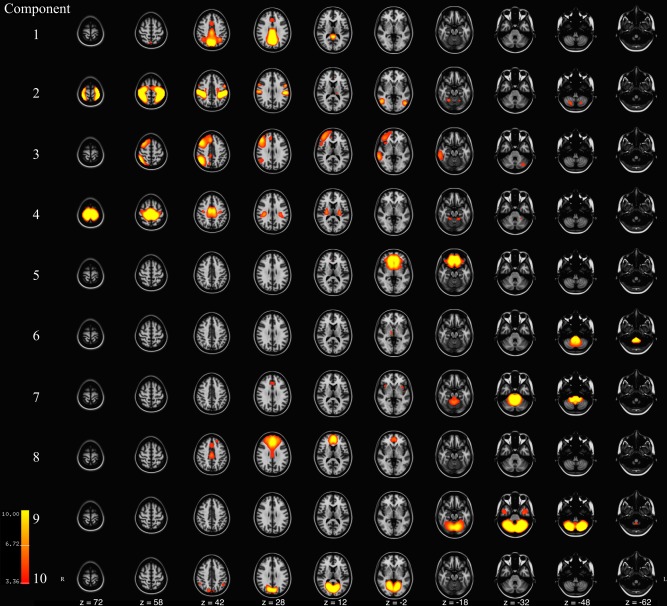
Axial slices of components 1‐to‐10 resulting from meta ICA of 500 repeated ICA samples. Components are thresholded at z = 3.09 (P < 0.001). Component Labels: 1 = Default Mode Network I, 2 = Sensory, 3 = Right Frontoparietal, 4 = Sensorimotor, 5 = Inferior Frontal, 6 = Lower Brainstem, 7 = Brainstem, 8 = Middle Frontal, 9 = Cerebellar, 10 = Anterior Visual. [Color figure can be viewed at http://wileyonlinelibrary.com]

Figure 2.

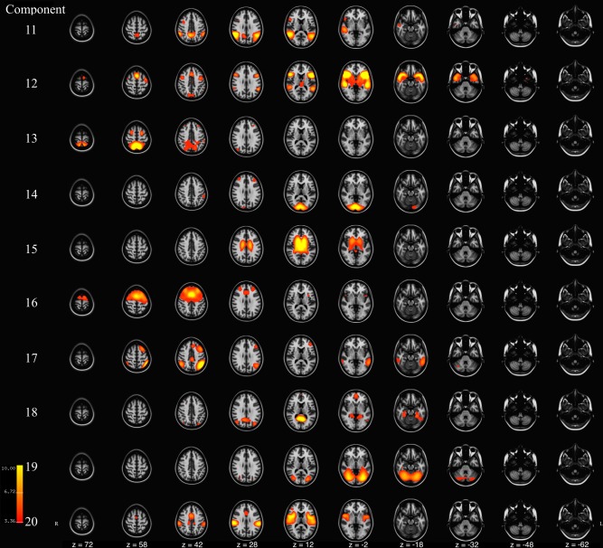
Axial slices of components 11‐to‐20 resulting from meta ICA of 500 repeated ICA samples. Components are thresholded at z = 3.09 (P < 0.001). Component Labels: 11 = Precuneus, 12 = Lateral Frontal, 13 = Parietal, 14 = Visual, 15 = Ventricular, 16 = Executive Control, 17 = Left Frontoparietal, 18 = Default Mode Network II, 19 = Cerebellar‐Occipital, 20 = Insular. [Color figure can be viewed at http://wileyonlinelibrary.com]

Figure 3.

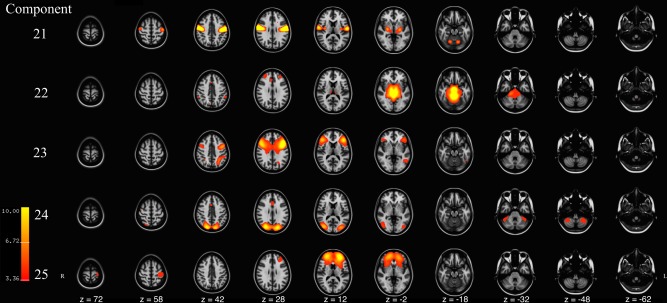
Axial slices of components 21–25 resulting from meta ICA of 500 repeated ICA samples. Components are thresholded at z = 3.09 (P < 0.001). Component Labels: 21 = Motor, 22 = Upper Brainstem, 23 = Frontal‐temporal‐Parietal, 24 = Lateral Visual, 25 = Lateral Middle Frontal. [Color figure can be viewed at http://wileyonlinelibrary.com]

Table 2.

Descriptive information of meta‐ICA derived components

Component	Functional label	Anatomical labels	0.1 Hz power ratio
1	DMN‐I	Precuneus, Cingulate‐PD, Lat. Occipital‐SD, Cingulate‐AD, Cuneous, Paracingulate, Sup. Parietal, Angular	0.33 ± 0.04
2	Sensory	Postcentral, Precentral, Sup. Parietal, Supramarginal‐AD, Lat. Occipital‐ID, Lat. Occipital‐SD, Sup. Frontal, Supramarginal‐PD, Juxtapositional, Mid. Frontal, Mid. Temporal	0.46 ± 0.08
3	R. Frontoparietal	Frontal Pole, Mid. Frontal, Lat. Occipital‐SD, Sup. Frontal, Angular, Mid. Temporal‐PD, Sup. Parietal, Supramarginal‐PD, Paracingulate, Precentral, Mid. Temporal, Pars Opercularis, Inf. Temporal, Cingulate‐PD, Sup. Temporal‐PD	0.38 ± 0.05
4	Sensorimotor	Precentral, Postcentral, Juxtapositional, Cingulate‐PD, Sup. Parietal, Precuneus, Sup. Frontal, Parietal Operculum, Cingulate‐AD	0.54 ± 0.10
5	Inf. Frontal	Frontal Pole, Orbital Frontal, Subcallosal, Med. Frontal, Paracingulate, Cingulate‐AD, L. Putamen, R. Putamen, R. Caudate, L. Caudate	0.71 ± 0.10
6	Lower Brainstem	Brainstem, R. Thalamus	0.90 ± 0.10
7	Brainstem	Brainstem, Insular, Cingulate‐AD	0.90 ± 0.08
8	Mid. Frontal	Frontal Pole, Paracingulate, Cingulate‐AD, Cingulate‐PD, Sup. Frontal, Mid. Frontal	0.66 ± 0.18
9	Cerebellar	Temporal‐Occipital Fusiform, Occipital Fusiform, Lingual, Temporal Fusiform‐PD, Inf. Temporal‐AD	0.91 ± 0.11
10	Ant. Visual	Lingual, Precuneus, Intracalcarine, Cuneous, Occipital Fusiform, Lat. Occipital‐SD, Angular, Temporal‐Occipital Fusiform, Supracalcarine, Cingulate‐PD, Occipital Pole	0.56 ± 0.09
11	Precuneus	Precuneus, Angular, Lat. Occipital‐SD, Supramarginal‐PD, Mid. Temporal, Sup. Temporal‐PD, Lat. Occipital‐ID, Mid. Temporal‐PD, Pars Opercularis, Mid. Frontal, Supramarginal‐AD	0.47 ± 0.09
12	Lat. Frontal	Temporal Pole, Orbital Frontal, Insular, Precentral, Sup. Temporal‐PD, Pars Opercularis, Mid. Temporal‐PD, Mid. Frontal, Sup. Frontal, L. Thalamus, Pars Triangularis, Supramarginal‐PD, Paracingulate, Planum Polare, L. Putamen, R. Thalamus, Frontal Operculum, Mid. Temporal‐AD, Mid. Temporal, Angular, R. Putamen, Sup. Temporal‐AD, Temporal Fusiform‐AD, Juxtapositional, Central Opercular	0.46 ± 0.07
13	Parietal	Lat. Occipital‐SD, Precuneus, Sup. Parietal, Postcentral, Sup. Frontal, Mid. Frontal, Frontal Pole	0.45 ± 0.07
14	Visual	Occipital Pole, Lingual Gyrus, Intracalcarine, Occipital Fusiform, Lat. Occipital‐ID, Frontal Pole, Supramarginal‐AD, Mid. Frontal, Cuneous, Supracalcarine, Lat. Occipital‐SD	0.63 ± 0.10
15	Ventricular	R. Thalamus, L. Thalamus, L. Lat. Ventricle, R. Lat. Ventricle, R. Putamen, L. Putamen, R. Caudate, L. Caudate, L. Pallidum, R. Pallidum, Insular	0.64 ± 0.11
16	Executive Control	Sup. Frontal, Mid. Frontal, Precentral, Frontal Pole, Juxtapositional, Paracingulate, Cingulate‐AD	0.64 ± 0.14
17	L. Frontoparietal	Lat. Occipital‐SD, Mid. Frontal, Angular, Mid. Temporal‐PD, Sup. Frontal, Supramarginal‐PD, Inf. Temporal, Mid. Temporal, Sup. Parietal, Cingulate‐PD, Inf. Temporal‐PD, Supramarginal‐AD, Frontal Pole, Paracingulate	0.39 ± 0.06
18	DMN‐II	Precuneus, Lat. Occipital‐SD, Cingulate‐PD, Lingual, Paracingulate, Temporal‐Occipital Fusiform, Frontal Pole, Inf. Temporal, Temporal Fusiform‐PD, R. Hippocampus, L. Hippocampus, Parahippocampal‐PD, Intracalcarine	0.33 ± 0.06
19	Cerebelum‐Occ.	Lat. Occipita‐ID, Lingual, Occipital Fusiform, Temporal‐Occipital Fusiform, Inf. Temporal, Lat. Occipital‐SD, Mid. Temporal	0.83 ± 0.14
20	Insular	Central Opercular, Supramarginal‐AD, Insular, Parietal Operculum, Cingulate‐AD, Planum Temporale, Precentral, Supramarginal‐PD, Postcentral, Heschl's, Juxtapositional, Frontal Operculum, Paracingulate, Planum Polare, Sup. Temporal‐PD, R. Putamen, L. Putamen, Pars Opercularis.	0.48 ± 0.07
21	Motor	Precentral, Postcentral, Cent. Opercular, L. Thalamus, R. Putamen, L. Putamen, R. Thalamus, Insular	0.46 ± 0.06
22	Upper Brainstem	Brainstem, L. Thalamus, R. Thalamus, Parahippocampal‐PD, Lingual, R. Hippocampus, L. Hippocampus, Frontal Pole, Paracingulate, Parahippocampal‐AD, R. Pallidum, L. Pallidum, R. Putamen, Temporal Fusiform‐PD	0.88 ± 0.11
23	Frontal‐Temporal‐Parietal	Mid. Frontal, Frontal Pole, Precentral, Pars Opercularis, Pars Triangularis, Lat. Occipital‐SD, Sup. Parietal, Orbital Frontal, Frontal Operculum, Inf. Temporal, Cingulate‐AD	0.40 ± 0.08
24	Lateral Visual	Lat. Occipital‐SD, Lat. Occipital‐ID, Cuneous, Occipital Pole, Precuneus, Cingulate‐AD	0.59 ± 0.10
25	Lat. Mid. Frontal	Frontal Pole, Paracingulate, Cingulate‐AD, Poscentral, Insular, Precentral, Frontal Operculum, L. Caudate, L. Putamen, R. Caudate	0.81 ± 0.17

Note: Component numbers correspond to those used in other figures. Anatomical labels are ordered according to their overlap with the component, in decending order. Abbreviations; AD, anterior division; Inf, inferior; ID, inferior division; Lat, lateral; L, left; Mid, middle; PD, posterior division; Sup, Superior; SD, superior division; R, right.

Distribution of Components from Subsampling

Certain RS‐FMRI ICA networks appear in the literature frequently, while others are less frequently reported. In addition to defining ICA networks in young children, we aimed to also describe the frequency of which these components appear after repeated subsampling of the data. Each of 12,500 components resulting from the 500 subsamples was classified as one of the 25 meta‐ICA components, or as a unique component not represented in the 25 meta‐ICA components. To classify the components, set theory was used to label components based on spatial overlap [White et al., 2014]. In total, 35 components were identified; 25 meta‐ICA components (Figs. 1, 2, 3), plus an additional 10 components (Supporting Information Fig. II) that were not in the meta‐ICA set. Components represented in figures are numbered and ordered according to the times present (%) in resamples, which is depicted in histogram format in Figure 4. As can be seen, components 1‐to‐10 were present in 96% or more of the ICA resamples, components 11‐to‐14 were present in 91% or more of the ICA resamples, and components 15‐to‐22 were present in 77% or more of the ICA resamples. These included components frequently reported in the literature, including the cerebellar, default‐mode, executive control, frontoparietal, parietal, sensorimotor, and visual networks. However, other components were present in substantially fewer ICA resamples. Component 24, a visual area component, was only present in roughly 50% of the resamples. Further, component 30 (Supporting Information Fig. II), a parietal component previously reported in the literature, was only present in 21% of the ICA resamples. Interestingly, in addition to components often considered true RSNs (e.g., the DMN), components with a spatial distribution and power spectrum likely attributable to noise are still present in 98% of the subsamples. For example, this is the case in two brainstem components (components 6 and 7) that are potentially related to physiological noise. However, some of these “noise” components occurred less frequently, including a frontal component indicative of motion (component 26) and a component related to white matter signal (component 31, see Supporting Information Fig. II). Given features of the histogram presented in Figure 4, it is possible to classify components as robust or variable based on “drop offs” in the frequencies depicted in the histogram. For instance, components 1 through 9 could be considered highly robust, and components 10 through 22 could be considered robust. However, given the relatively steep decrease in observed frequency at component 23, components 23 through 35 could be considered more variable.

Figure 4.

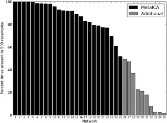
Frequencies (presence) of components observed after repeated ICA subsampling. Components observed in only the meta‐ICA (black), and those found in repeated subsamples but not represented in the meta‐ICA (gray) are shown.

The spatial variability in components across resamples was explored using a voxel‐wise 1‐sample t‐test on all matched components (P _FWE < 0.05). Supporting Information Figure III illustrates these maps in the 25 meta‐ICA components. As can be seen, there is high overlap in the center of most nodes of the components across the 500 ICA runs (see corresponding meta‐ICA components in Figs. 1, 2, 3). Interestingly, lower overlap across the 500 ICA runs is apparent in certain nodes of components that split into separate/distinct components with higher dimensionality (e.g., the frontal node of the DMN).

Within‐Network Associations with Age

Results from voxel‐wise statistics on subject‐specific component maps from Dual Regression are presented in Figure 5. For the DMN, a negative association with age was observed in the precuneus/posterior cingulate node. Similarly, for the executive control network, a negative correlation was observed in the frontal and anterior cingulate aspects of the network. In the right front‐parietal network, a positive association with age is observed in the left hemisphere, mainly in the insula and temporal lobe. No significant associations were observed between age and the left frontoparietal network after adjusting for confounders and multiple testing.

Figure 5.

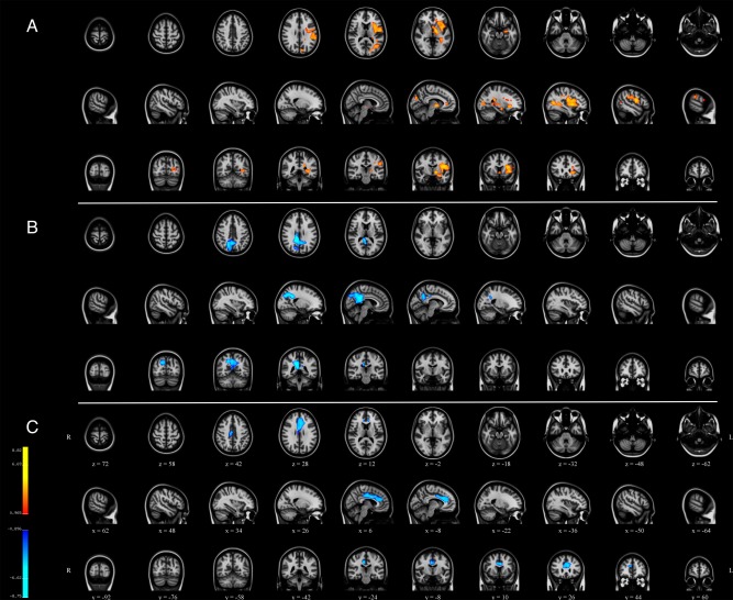
Within‐network associations with age using spatiotemporal regression. Clusters are t‐values indicating significant association at P _corrected < 0.05, with red indicating a positive association with age and blue indicating a negative association with age. (a) meta‐ICA component 3/right frontoparietal, (b) meta‐ICA component 1/default mode network, and (c) meta‐ICA component 16/executive control network. [Color figure can be viewed at http://wileyonlinelibrary.com]

Between‐Network Associations with Age

Regression analyses of between‐network connectivity revealed that the correlation between Component 11 (Precuneus) and Component 12 (Lateral Frontal) was positively associated with age (β = 0.20, P _FWE = 0.0004). Thus, the correlation between these networks was stronger (becoming more positive) in older children (Fig. 6). Further, the correlation between Component 3 (Right Frontoparietal) and Component 13 (Parietal) and was negatively associated with age (β = −0.17, P _FWE = 0.0056). In older children, the correlation between these networks is lower (becoming more negative, Fig. 6). Lastly, the correlation between Component 2 (Sensory) and Component 3 (Right Frontoparietal) was negatively associated with age (β = −0.15, P _FWE = 0.027).

Figure 6.

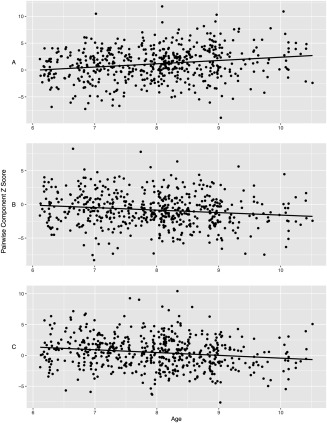
Between‐network associations with age. The x‐axis reflects age in years and the y‐axis is the pairwise correlations between time courses of two components, transformed to the Z distribution. A = Components 11 and 12, B = Components 3 and 13, and C = Components 2 and 3.

DISCUSSION

The present study examines resting‐state FMRI networks in a large sample of 6‐to‐10 year old children using independent component analyses. A subsampling approach was used to generate a representative set of components, and to identify robustness of components across repeated ICA runs. The subsampling revealed that many components commonly reported in the literature show a high level of stability across repeated sampling. Further, many of the components that are typically identified in studies of adults were also found in the current sample of young children. Interestingly, networks believed to be the result of noise and/or artifacts were also observed at frequencies similar to true RSNs after iterative ICA subsampling. Lastly, even within a very narrow age‐range, the study demonstrated age‐related associations with various networks, suggesting continued refinement of networks is occurring during childhood.

The subsampling procedure used in the current study highlights important characteristics of RS‐FMRI ICA analyses, namely that many components are quite robust. This is true for both what is considered RSNs and for “noise” signals. Previous studies have already discussed issues surrounding ICA, for example variability related to subject order or ICA reliability [Franco et al., 2013; Himberg et al., 2004; Zhang et al., 2010]. In the present study we expand upon this showing that many components typically characterized in the literature as RSNs were observed frequently across the repeated ICA runs (e.g., the DMN, sensory, motor, and frontoparietal networks). While these results do not give a clear indication of the precise reliability of the spatial extent of the various components, they do demonstrate that many components from ICA can be repeatedly extracted from RS‐FMRI data in young children, despite variability in the sample and algorithm‐dependent variability in ICAs. The data also show that components suggestive of noise in RS‐FMRI data (e.g., resulting from hardware, physiological, image analysis, etc.) can be reliably detected in children using ICA. For example, components 6 and 7 (both part of the brainstem) were present in over 98% of the repeated ICA analyses.

However, given that certain components were not observed as frequently as others (i.e., roughly 55% of the time or less), it is prudent to critically evaluate these components in future studies (for instance, components 29 and 30). This may be especially important in ICA‐derived components considered to be RSNs and subjected to further analysis using the myriad of methods available [e.g., spatiotemporal regression, backwards‐reconstruction, seed‐based, etc. Calhoun et al., 2008; Filippini et al., 2009; Tian et al., 2013], to ensure they are not simply artifacts of the data or image analysis algorithm. It is however interesting to consider the possibility that some of these less frequently occurring components are not artifact or algorithm‐dependent, but rather arise from other sources. For instance, the variability could reflect individual differences in RS‐FMRI networks in typically developing children [Michael et al., 2014]. If such individual differences exist and can be observed, those components could offer further insight into brain development, various neurological or psychiatric disorders, or in the fields of social or behavioral neuroscience. Conversely, while the age‐range in the current study is comparatively narrow compared with many studies of brain development, it is possible that the observed variability in components is simply age‐related. For instance, networks not present in all resamples could be subject to neurodevelopment processes that later stabilize in adulthood. Thus, generalizations to other age‐ranges should be made carefully and similar analyses should be explored in adolescents and young adults, or preferably, networks should be tracked using longitudinal designs.

While not traditionally done in the existing literature, the current study also presents components that are typically labeled as “noise” or “other” and discarded from analyses. Many components that are likely attributable to noise actually were very robust in repeated sampling. This suggests that many noise signals are present in different subject groups and that ICA can reliably detect them. This information also hopefully gives other groups a point of reference when examining group ICA components, and also may help future work in deciding which of these components are generalizable across studies, and which are not (i.e., those that are MR‐scanner dependent, sequence dependent, etc.). It is unclear how useful this information will be across studies, as some of the noise components were highly variable, and could be related to the scanner hardware, thermal noise, or even the performance of the ICA‐based artifact removal. However, while beyond the scope of the current study, the repeated subsampling results with and without the subject‐level ICA denoising step were run and produced group meta‐ICA results similar to those reported in the current study (Supporting Information Fig. IV). This is particularly interesting given the increased attention surrounding pediatric imaging with respect to motion confounds. However, while the cleanup procedure may only marginally influence the results of group ICA, it has been previously shown to influence other important aspects of analyses, such as spatiotemporal regression, and thus should not be considered unnecessary [Mowinckel et al., 2012; Satterthwaite et al., 2012].

Age‐related associations within the DMN revealed the central, posterior cingulate/precuneus node of the default mode network to be negatively correlated with age, after adjusting for sex, behavioral problems, and ethnicity. This observation was previously only reported in adults, where a highly similar spatial pattern of aging rather than developmental effects was observed in individuals 21‐to‐81 years of age using spatiotemporal regression [Mowinckel et al., 2012]. We also observed a positive association between age and the contralateral hemisphere of the right frontoparietal network, suggesting a potential increase in interhemispheric communication with age. Lastly, between network analyses revealed that certain networks (i.e., the precuneus and lateral frontal) become more strongly connected with increasing age, whereas other networks become less strongly connected with age (e.g., the right frontoparietal and sensory). These results taken together are particularly intriguing, given they demonstrate evidence for maturation of functional connectivity in a very narrow age‐range.

Another aspect worthy of discussion is the study sample. In the extant literature, it is relatively clear, and occasionally noted, that the labels “typically developing” or “normal” are at times somewhat misleading. Studies of normative brain development often times experience selection bias, including children with higher than average IQ and social economic status. Further, diversity in ethnic background tends to be limited, and the prevalence of behavioral problems in these samples is likely lower than what would be observed in a true random sampling of the population. A similar scenario has been considered in the context of case‐control studies [Schwartz and Susser, 2011]. In the current study, the children were sampled from a population‐based cohort. Importantly, severe behavioral problems were an exclusion criteria, and thus the sample is not truly representative at the population level. However, other aspects of the study sample, including non‐verbal IQ show close correspondence with the population average (current study mean = 103, population average = 100). Further, ethnicity in the current sample was fairly representative of the catchment area, with roughly 17% of the sample was of non‐Western decent. These factors, when taken together, suggest the current sample is less representative of a “hyper‐normal” group and more representative of the overall population compared many studies of typical brain development.

In addition to describing RSNs in children, another goal of the present study was to facilitate replication and generalizability in RS‐FMRI data analyses. Thus, the final set of meta‐ICA spatial maps have been made available under a non‐commercial license to the neuroimaging community via the Neuroimaging Informatics Tools and Resources Clearinghouse (NITRC) website (http://www.nitrc.org/projects/genr/). Interested researchers are able to utilize the components to aid in their research efforts, for example, in comparison against those identified in their own studies, for use in spatial‐temporal regression (dual regression), or as an “atlas” for reference with other RS‐FMRI ICA studies, task‐based FMRI studies and structural neuroimaging studies. Further, the age‐appropriate T₁‐weighted brain described in section “Study‐specific, age‐appropriate template for registration” is also available for those interested in a pediatric structural brain for registration.

While the current study has many strengths, some limitations are present and deserve attention. First, the current study presents independent component analyses of resting‐state data in children, imposing a dimensionality of 25. While it is highly unlikely 25 components represent the true set of RSNs in the brain, this number was chosen because it fits well with the existing literature and generates a similar set of components to what has been presented previously in both child, adolescent and adult studies. With increasing spatial and temporal resolution of acquired RS‐FMRI data, using higher dimensionalities becomes more feasible, even though it has been observed that increasing the dimensionality may actually simply split components into sub‐networks [Smith et al., 2009]. There is also interesting evidence from large studies suggesting the brain is organized into a relatively low number of networks [Yeo et al., 2011]. While noise components are reported in the current study, and it is likely that some of them will be generalizable (i.e., replicate) across studies/research groups, some of these noise components will not be generalizable. For example, certain components could be related to a particular MR‐scanner profile, which may or may not even replicate within a given model/manufacturer of scanner [Friedman et al., 2008]. However, some of these components (e.g., those related to respiratory and cardiac physiology) will most likely be applicable across site, and it will be interesting to see how they compare to components other groups observe. Lastly, while the current study did investigate the frequency components were observed after repeated subsampling, it was beyond the scope of the study to examine the spatial variability of the components in detail. Future studies may wish to examine this, perhaps in the context of higher and lower dimensionality.

The current study presents evidence that many RSNs in young children are quite robust, occurring frequently under repeated ICAs, while other RSNs are less frequently observed and require additional scrutiny when involving between‐group comparisons. Further, these components demonstrate age‐related associations, suggesting they are sensitive to subtle developmental changes. The final meta‐ICA group components and pediatric T₁‐weighted structural template are made available to the neuroimaging community for research purposes (https://www.nitrc.org/projects/genr/).

Supporting information

Supporting Information Figure 1.

Supporting Information Figure 2.

Supporting Information Figure 3.

Supporting Information Figure 4.

REFERENCES

- Achenbach TM, Rescorla LA (2000): Manual for ASEBA preschool forms & profiles. Burlington, VT: University of Vermont, Research Center for Children, Youth & Families. [Google Scholar]
- Achenbach TM, Ruffle TM (2000): The Child Behavior Checklist and related forms for assessing behavioral/emotional problems and competencies. Pediatr Rev/Am Acad Pediatr 21:265–271. [DOI] [PubMed] [Google Scholar]
- Beckmann CF, DeLuca M, Devlin JT, Smith SM (2005): Investigations into resting‐state connectivity using independent component analysis. Philos Trans R Soc Lond Ser B, Biol Sci 360:1001–1013. [DOI] [PMC free article] [PubMed] [Google Scholar]
- Biswal BB, Mennes M, Zuo XN, Gohel S, Kelly C, Smith SM, Beckmann CF, Adelstein JS, Buckner RL, Colcombe S, Dogonowski AM, Ernst M, Fair D, Hampson M, Hoptman MJ, Hyde JS, Kiviniemi VJ, Kotter R, Li SJ, Lin CP, Lowe MJ, Mackay C, Madden DJ, Madsen KH, Margulies DS, Mayberg HS, McMahon K, Monk CS, Mostofsky SH, Nagel BJ, Pekar JJ, Peltier SJ, Petersen SE, Riedl V, Rombouts SA, Rypma B, Schlaggar BL, Schmidt S, Seidler RD, Siegle GJ, Sorg C, Teng GJ, Veijola J, Villringer A, Walter M, Wang L, Weng XC, Whitfield‐Gabrieli S, Williamson P, Windischberger C, Zang YF, Zhang HY, Castellanos FX, Milham MP (2010): Toward discovery science of human brain function. Proc Natl Acad Sci U S A 107:4734–4739. [DOI] [PMC free article] [PubMed] [Google Scholar]
- Calhoun VD, Adali T, Pearlson GD, Pekar JJ (2001): A method for making group inferences from functional MRI data using independent component analysis. Hum Brain Mapp 14:140–151. [DOI] [PMC free article] [PubMed] [Google Scholar]
- Calhoun VD, Maciejewski PK, Pearlson GD, Kiehl KA (2008): Temporal lobe and “default” hemodynamic brain modes discriminate between schizophrenia and bipolar disorder. Hum Brain Mapp 29:1265–1275. [DOI] [PMC free article] [PubMed] [Google Scholar]
- Cole DM, Smith SM, Beckmann CF (2010): Advances and pitfalls in the analysis and interpretation of resting‐state FMRI data. Front Syst Neurosci 4:8. [DOI] [PMC free article] [PubMed] [Google Scholar]
- Damoiseaux JS, Rombouts SA, Barkhof F, Scheltens P, Stam CJ, Smith SM, Beckmann CF (2006): Consistent resting‐state networks across healthy subjects. Proc Natl Acad Sci U S A 103:13848–13853. [DOI] [PMC free article] [PubMed] [Google Scholar]
- de Bie HM, Boersma M, Adriaanse S, Veltman DJ, Wink AM, Roosendaal SD, Barkhof F, Stam CJ, Oostrom KJ, Delemarre‐van de Waal HA, Sanz‐Arigita EJ (2012): Resting‐state networks in awake five‐ to eight‐year old children. Hum Brain Mapp 33:1189–1201. [DOI] [PMC free article] [PubMed] [Google Scholar]
- Desikan RS, Segonne F, Fischl B, Quinn BT, Dickerson BC, Blacker D, Buckner RL, Dale AM, Maguire RP, Hyman BT, Albert MS, Killiany RJ (2006): An automated labeling system for subdividing the human cerebral cortex on MRI scans into gyral based regions of interest. Neuroimage 31:968–980. [DOI] [PubMed] [Google Scholar]
- Filippini N, MacIntosh BJ, Hough MG, Goodwin GM, Frisoni GB, Smith SM, Matthews PM, Beckmann CF, Mackay CE (2009): Distinct patterns of brain activity in young carriers of the APOE‐epsilon4 allele. Proc Natl Acad Sci U S A 106:7209–7214. [DOI] [PMC free article] [PubMed] [Google Scholar]
- Franco AR, Mannell MV, Calhoun VD, Mayer AR (2013): Impact of analysis methods on the reproducibility and reliability of resting‐state networks. Brain Connect 3:363–374. [DOI] [PMC free article] [PubMed] [Google Scholar]
- Friedman L, Stern H, Brown GG, Mathalon DH, Turner J, Glover GH, Gollub RL, Lauriello J, Lim KO, Cannon T, Greve DN, Bockholt HJ, Belger A, Mueller B, Doty MJ, He J, Wells W, Smyth P, Pieper S, Kim S, Kubicki M, Vangel M, Potkin SG (2008): Test‐retest and between‐site reliability in a multicenter fMRI study. Hum Brain Mapp 29:958–972. [DOI] [PMC free article] [PubMed] [Google Scholar]
- Gao W, Zhu H, Giovanello KS, Smith JK, Shen D, Gilmore JH, Lin W (2009): Evidence on the emergence of the brain's default network from 2‐week‐old to 2‐year‐old healthy pediatric subjects. Proc Natl Acad Sci U S A 106:6790–6795. [DOI] [PMC free article] [PubMed] [Google Scholar]
- Griffanti L, Salimi‐Khorshidi G, Beckmann CF, Auerbach EJ, Douaud G, Sexton CE, Zsoldos E, Ebmeier KP, Filippini N, Mackay CE, Moeller S, Xu J, Yacoub E, Baselli G, Ugurbil K, Miller KL, Smith SM (2014): ICA‐based artefact removal and accelerated fMRI acquisition for improved resting state network imaging. Neuroimage 95:232–247. [DOI] [PMC free article] [PubMed] [Google Scholar]
- Himberg J, Hyvarinen A, Esposito F (2004): Validating the independent components of neuroimaging time series via clustering and visualization. Neuroimage 22:1214–1222. [DOI] [PubMed] [Google Scholar]
- Jaddoe VW, van Duijn CM, Franco OH, van der Heijden AJ, van Iizendoorn MH, de Jongste JC, van der Lugt A, Mackenbach JP, Moll HA, Raat H, Rivadeneira F, Steegers EA, Tiemeier H, Uitterlinden AG, Verhulst FC, Hofman A (2012): The Generation R Study: Design and cohort update 2012. Eur J Epidemiol 27:739–756. [DOI] [PubMed] [Google Scholar]
- Jenkinson M, Beckmann CF, Behrens TE, Woolrich MW, Smith SM (2012): Fsl. Neuroimage 62:782–790. [DOI] [PubMed] [Google Scholar]
- Jolles DD, van Buchem MA, Crone EA, Rombouts SA (2011): A comprehensive study of whole‐brain functional connectivity in children and young adults. Cereb Cortex 21:385–391. [DOI] [PubMed] [Google Scholar]
- Langeslag SJ, Schmidt M, Ghassabian A, Jaddoe VW, Hofman A, van der Lugt A, Verhulst FC, Tiemeier H, White TJ (2012): Functional connectivity between parietal and frontal brain regions and intelligence in young children: The Generation R study. Hum Brain Mapp 34:3299–3307. [DOI] [PMC free article] [PubMed] [Google Scholar]
- Littow H, Elseoud AA, Haapea M, Isohanni M, Moilanen I, Mankinen K, Nikkinen J, Rahko J, Rantala H, Remes J, Starck T, Tervonen O, Veijola J, Beckmann C, Kiviniemi VJ (2010): Age‐related differences in functional nodes of the brain cortex ‐ a high model order group ica study. Front Syst Neurosci 4:32. [DOI] [PMC free article] [PubMed] [Google Scholar]
- Michael AM, Anderson M, Miller RL, Adali T, Calhoun VD (2014): Preserving subject variability in group fMRI analysis: Performance evaluation of GICA vs. IVA. Front Syst Neurosci 8:106. [DOI] [PMC free article] [PubMed] [Google Scholar]
- Mowinckel AM, Espeseth T, Westlye LT (2012): Network‐specific effects of age and in‐scanner subject motion: A resting‐state fMRI study of 238 healthy adults. Neuroimage 63:1364–1373. [DOI] [PubMed] [Google Scholar]
- Power JD, Barnes KA, Snyder AZ, Schlaggar BL, Petersen SE (2012): Spurious but systematic correlations in functional connectivity MRI networks arise from subject motion. Neuroimage 59:2142–2154. [DOI] [PMC free article] [PubMed] [Google Scholar]
- Salimi‐Khorshidi G, Douaud G, Beckmann CF, Glasser MF, Griffanti L, Smith SM (2014): Automatic denoising of functional MRI data: Combining independent component analysis and hierarchical fusion of classifiers. Neuroimage 90:449–468. [DOI] [PMC free article] [PubMed] [Google Scholar]
- Sanchez CE, Richards JE, Almli CR (2012): Age‐specific MRI templates for pediatric neuroimaging. Dev Neuropsychol 37:379–399. [DOI] [PMC free article] [PubMed] [Google Scholar]
- Satterthwaite TD, Wolf DH, Loughead J, Ruparel K, Elliott MA, Hakonarson H, Gur RC, Gur RE (2012): Impact of in‐scanner head motion on multiple measures of functional connectivity: Relevance for studies of neurodevelopment in youth. Neuroimage 60:623–632. [DOI] [PMC free article] [PubMed] [Google Scholar]
- Schwartz S, Susser E (2011): The use of well controls: An unhealthy practice in psychiatric research. Psychol Med 41:1127–1131. [DOI] [PubMed] [Google Scholar]
- Smith SM, Nichols TE (2009): Threshold‐free cluster enhancement: Addressing problems of smoothing, threshold dependence and localisation in cluster inference. Neuroimage 44:83–98. [DOI] [PubMed] [Google Scholar]
- Smith SM, Fox PT, Miller KL, Glahn DC, Fox PM, Mackay CE, Filippini N, Watkins KE, Toro R, Laird AR, Beckmann CF (2009): Correspondence of the brain's functional architecture during activation and rest. Proc Natl Acad Sci U S A 106:13040–13045. [DOI] [PMC free article] [PubMed] [Google Scholar]
- Tian L, Kong Y, Ren J, Varoquaux G, Zang Y, Smith SM (2013): Spatial vs. temporal features in ica of resting‐state fmri ‐ a quantitative and qualitative investigation in the context of response inhibition. PLoS One 8:e66572. [DOI] [PMC free article] [PubMed] [Google Scholar]
- Tick NT, van der Ende J, Koot HM, Verhulst FC (2007): 14‐year changes in emotional and behavioral problems of very young Dutch children. J Am Acad Child Adolesc Psychiatry 46:1333–1340. [DOI] [PubMed] [Google Scholar]
- Tiemeier H, Velders FP, Szekely E, Roza SJ, Dieleman G, Jaddoe VW, Uitterlinden AG, White TJ, Bakermans‐Kranenburg MJ, Hofman A, Van Ijzendoorn MH, Hudziak JJ, Verhulst FC (2012): The Generation R Study: A review of design, findings to date, and a study of the 5‐HTTLPR by environmental interaction from fetal life onward. J Am Acad Child Adolesc Psychiatry 51:1119–1135 e7. [DOI] [PubMed] [Google Scholar]
- White T, El Marroun H, Nijs I, Schmidt M, van der Lugt A, Wielopolki PA, Jaddoe VW, Hofman A, Krestin GP, Tiemeier H, Verhulst FC (2013): Pediatric population‐based neuroimaging and the Generation R Study: The intersection of developmental neuroscience and epidemiology. Eur J Epidemiol 28:99–111. [DOI] [PubMed] [Google Scholar]
- White T, Muetzel R, Schmidt M, Langeslag SJ, Jaddoe V, Hofman A, Calhoun VD, Verhulst FC, Tiemeier H (2014): Time of acquisition and network stability in pediatric resting‐state functional MRI. Brain Connect 4:417–427. [DOI] [PMC free article] [PubMed] [Google Scholar]
- Winkler AM, Ridgway GR, Webster MA, Smith SM, Nichols TE (2014): Permutation inference for the general linear model. Neuroimage 92:381–397. [DOI] [PMC free article] [PubMed] [Google Scholar]
- Yeo BT, Krienen FM, Sepulcre J, Sabuncu MR, Lashkari D, Hollinshead M, Roffman JL, Smoller JW, Zollei L, Polimeni JR, Fischl B, Liu H, Buckner RL (2011): The organization of the human cerebral cortex estimated by intrinsic functional connectivity. J Neurophysiol 106:1125–1165. [DOI] [PMC free article] [PubMed] [Google Scholar]
- Zhang H, Zuo XN, Ma SY, Zang YF, Milham MP, Zhu CZ (2010): Subject order‐independent group ICA (SOI‐GICA) for functional MRI data analysis. Neuroimage 51:1414–1424. [DOI] [PubMed] [Google Scholar]
Associated Data
This section collects any data citations, data availability statements, or supplementary materials included in this article.
Supplementary Materials